Abstract
The present paper considers a model of stalling in a queueing system (QS) with any number of different capacities of heterogeneous servers. The state graph and the corresponding linear system for steady-state probabilities are derived using the standard Markov chain technique. The obtained solution of the steady-state probabilities model is numerically stable; the complexity of the corresponding expressions does not depend on the number of QS states; thus, they enable us to analytically study the QS characteristics. Optimization of a stalling buffer is considered as well, and it is shown that stalling helps us to solve the slow server problem under an appropriate choice of stalling buffer size, making the slow servers usable under various values of system load. The asymptotic conditions of optimal query distribution in channels, when the ratio of the capacities of the fast and slow servers is increasing, are also established. Moreover, some applications of the developed model in heterogeneous server clusters and in work productivity modelling for forest harvesting applications are discussed.
1. Introduction
Queueing systems (QSs) with different capacity channels are often used in technology and business. Usually, the theory of discrete Markov processes is used for QS modelling, and the probabilities of steady states are calculated from a linear equations system; here, the coefficients are equal to the rates of transition, while the order of the system is equal to the number of states [1]. If all channels of the linear system have the same capacity, this system has an analytical solution with a complexity that does not depend on the number of states. However, in general, this system of equations for the state probabilities of a QS with several heterogeneous channels can depend on the number of states, which might be significant, and it can be unstable.
The queueing strategies in QSs with two or several different channels have been analysed by many authors, see, for example [2,3,4,5,6,7,8,9,10,11]. Computer programs are developed to determine the optimal allocation of storage spaces among three heterogeneous servers, by calculating the bounds of sizes of finite sources for different traffic intensities [12]. Particular cases of the steady-state behaviour of a discrete-time queueing problem with S heterogeneous groups with a discipline FCFS and a limited waiting space were analysed in [13,14]; a set of heterogeneous and exponential servers were discussed in [15]. El-Taha and Stidham [16], using deterministic (sample-path) analysis, generalized and extended the fundamental properties of systems with “stationary deterministic flows”. They proved the renewal–reward theorem and established a relationship that shows that the “operational analysis” definition of average service times—when considered as the observation period —coincides with the standard definition of average service times for all stable queueing systems. Moreover, the equilibrium in a single-server queueing system with retrials and strategic timing of the customers was analysed in [17]. The systems modelled by M/M/n queues with heterogeneous servers and non-informed customers show that there is a value of arrival rate; below this, the slow server should not be used, and above which, it should be used [18]. A multi-server controllable queueing system with heterogeneous servers was considered in [19]; here, several monotonicity properties of optimal policies for such a system were proved. Efrosinin and Rykov studied [7] the queuing system with K heterogeneous servers using a heuristic approach. Efrosinin and Sctrik [20,21] showed that, in an M/M/K queue, the optimal threshold levels may also depend on the states of slower servers; however, this influence is negligible. In [22], a finite-source queueing system serving one class of customers and consisting of heterogeneous servers with unequal service intensities and of one common queue were investigated. The authors of [23] provided an analysis of the dependence of the convergence of experimental results on the type of distribution used by the system parameters in heterogeneous queueing resource system with an unlimited number. In [24], a multi-server infinite buffer queueing system with additional servers (assistants) providing help to the main servers when they encountered problems was analysed through multi-dimensional Markov chains. The authors of [25] analysed heterogeneous queues where servers differ not only in service rates but also in operating costs; they presented a simple heuristic solution.
The proposed that the solutions for systems of heterogeneous services can also be applied in specific tasks of computer networks and multiprocessor systems in addition to solving social tasks and others. Heterogeneous server problems occur in multiprocessor systems, which combine CPU and GPU processors [26,27,28,29,30]. Expressions of the queue length distributions of the GPS and individual traffic flows were presented in [31]. The Quality of Service (QoS) in different service classes with real-time and non-real-time traffic integration is an important issue in WiMAX systems; therefore, the authors of [32,33] proposed a cross-layer QoS support scheduling framework and a corresponding opportunistic scheduling algorithm to provide QoS support to the heterogeneous traffic in a single-carrier WiMAX point-to-multipoint (PMP) system. The presented model is applied to the uplink transmission in the single-carrier WiMAX system as a multi-class priority TDMA queueing system in order to analyse the average packet delays of different service classes. The authors of [34] demonstrated that a processor’s fast cores may not be ideal for system workloads and that less can be more in some situations. Furthermore, in [35], a novel fuzzy testing technique, HFuzz, was proposed as a solution enabling efficient testing on real heterogeneous architectures. Research results showed that such a system can perform well, using much more constrained resources than are usually available.
This paper aims to show that stalling is an efficient approach for exploiting and managing heterogeneous systems. The model of stalling in QSs with two heterogeneous servers has been considered in [9] by the first two authors of this paper, where the explicit probabilities of steady states were derived. The results showed that the appropriate choice of stalling buffer size is helpful in solving the slow server problem. The asymptotic approximations of optimal stalling buffer size, when the ratio of the capacities of fast and slow servers is increasing, have also been established. The application of the model developed in computer networks has been discussed as well. Investigation of the developed model enables us to conclude that stalling is a universal solution which can be implemented into any heterogeneous system.
The findings presented in this paper for several-server QSs might be useful for the investigation of systems with any number of heterogeneous channels or servers with different capacities. Since the analytical study of systems with heterogeneous channels is rather complicated, a system with two types of servers, equipped with a stalling buffer and a finite waiting line, is presented and analysed.
2. QS with Heterogeneous Channels and Stalling Buffer
2.1. State Graph of QS
Let us consider a queueing system consisting of m + n heterogeneous channels, where m is the number of fast channels, n is the number of slow channels, K is the length of the stalling buffer, and M is the length of the waiting line and the buffer (see Figure 1). Assume that the interarrival time to the system is distributed exponentially with parameter λ and the service time is distributed also under this law with parameters µ1 and µ2, respectively, for fast and low channels, i.e., µ1 > µ2; the queries are served in the FCFS discipline. If the query—after being released into the system—finds a free fast channel, then it is served immediately; otherwise, it goes to a stalling buffer of K length, where it waits until the efficient channels become free. One query is served only by one channel without a break. If all the places in the stalling buffer are occupied, then the arrived query transfers to the slow channel. If the slow channel is occupied as well, then the application waits in the queue at a waiting buffer of length M. If all the places in the waiting and stalling buffers are occupied, then the query is rejected and it is deemed lost.
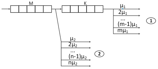
Figure 1.
Scheme of QS with stalling buffer.
The main parameter of the QS is the coefficient of utilization . Note, if the system is full (), then all the channels, i.e., slow and fast ones, should work because the service is most efficient if the system works at maximal capacity. If some channels work with idle time, then the system will process a smaller number of queries. If more queries come in than the system can serve, then unserved queries will be deemed lost, if the waiting line is finite.
2.2. Calculation of Steady-State Probabilities
Assume that the state of a QS with m + n heterogeneous channels, a stalling buffer of capacity K, and waiting line length M, be defined by numbers: , where i and j are the numbers of queries served in fast and slow channels, respectively, and k is the number of stalled or waiting queries—, , . Denote the corresponding steady-state probabilities by Pi,j,k. Let us draw the state graph of such a QS inn Figure 2; here, the vertexes denote the states connected by arrows representing transitions with non-null probability from one state to the other [1].
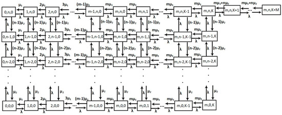
Figure 2.
Graph of QS state.
The states on the graph are specified as well:
P0,0,0—all channels and stalling buffers are free;
Pi,0,0—in the fast channels are the i queries, the slow channels and stalling buffer are free;
Pm,0,k—the fast channels are occupied with m queries, the slow channels are free, the k queries are stalled in the stalling bufferPm,0,K—the fast channels are occupied with m queries, the slow channels are free, the stalling buffer is full;
P0,j,0—in the slow channels are j queries, the fast channels and the stalling buffer are free;
Pi,j,0—in the fast channels are i queries, in the slow channels are j queries, the stalling buffer is free;
Pm,j,k —the fast channels are occupied with m queries, in the slow channels are j queries, k queries are stalled in the stalling buffer;
Pm,j,K—the fast channels are occupied with m queries, in the slow channels are j queries, the stalling buffer is full;
P0,n,0—only the slow channels are occupied with n queries;
Pi,n,0—in the fast channels are i queries, in the slow channels are n queries, the stalling buffer is free;
Pm,n,k—the fast channels are occupied with m queries, the slow channels are occupied with n queries, k queries are stalled in the stalling buffer;
Pm,n,k+K—the fast channels are occupied with m queries, the slow channels are occupied with n queries, the stalling buffer is full, k queries are waiting in line;
Pm,n,K+M—the fast channels are occupied with m queries, in the slow channels are n queries, the stalling buffer and the queue are full, and the next arrived query will be lost;
Typically, the probabilities of these states are calculated using a linear equation system whose coefficients are equal to the rates of transition while the order of the system is equal to the number of states [1]. Thus, one can derive steady-state equations according to the steady-state graph in Figure 2. They are given in the following system (1):
The obtained linear equation system is homogeneous; thus, the normalization condition is needed to ensure the uniqueness of the following solution:
The specific case of the steady-state system, when , is also given in [9]. Generally, the order of the linear equation system (1)–(2) is equal to the number of QS states . Note that solving this system using Cramer’s rule might become numerically complicated, because the implementation of this rule requires a third-order complexity algorithm from the number of states; in addition, this system is often is ill-posed.
Looking for a more simple, explicit solution led us to apply the following parameters to the characterization of a QS with a stalling buffer:
- Coefficient of utilization of fast servers with switched-out slow channels ;
- Rate of capacity of fast and slow servers
- Stalling buffer length K;
- Waiting queue length M.
Now, the coefficient of QS utilization is as follows:
Let us denote the polynomial functions and ratios that can be used to explicitly derive the steady-state probabilities from systems (1) and (2):
The explicit expressions of QS steady-state probabilities are given by Theorem A1.
Theorem A1.
Steady-state probabilities of QS with stalling, defined by system (1)–(2), are as follows, if :
Proof of Theorem A1 is given in Appendix A. For the proof of this theorem, we will use two Lemmas given below. Their proofs are also given in Appendix A.
Lemma A1.
The equalities exist as follows, if , , :
Lemma A2.
The ratios in (5) satisfy the recursive relation:
Remark.
Note that the sums , , according to the definition, are the steady-state probabilities of several queries in fast channels and the stalling buffer occupies both together. Using Lemma A1 and well-known formulas of steady-state probabilities in a multi-channel queueing system with the finite queue [1], we can easily make sure that these probabilities follow to the steady-state probabilities in an M/M/m/K system with a utilization coefficient q and queue length K:
3. Queuing Characteristics and Optimization
3.1. Queueing Characteristics
Probabilities (6)–(8) enable us to calculate the steady-state characteristics of multi-channel QS with stalling as probabilities of various QS states and numbers of queries in these states. Hence, one has at first to calculate the following, according to Lemmas A1 and A2: the × matrix of auxiliary functions ; components vector h, used to find the steady-state probabilities according to Theorem A1; and the other characteristics. Note, the obtained explicit expressions are numerically stable; in addition, their complexity does not depend on the number of states, and is only linear with respect to the number of fast channels and stalling buffer length. Some characteristics are given in Table 1, using the following notation for simplicity:

Table 1.
Characteristics of QS with stalling, .
A key characteristic of QS is the occupancy probability of all channels and stalling buffer only , derived according to Theorem A1. For calculating the characteristics using (6)–(10), the well-known Newton binomial formula is applied:
The explicitly given characteristics help us to study various effects; for instance, the effect of a query becoming stuck can be studied—the situation when the fast channels and the stalling buffer are free, but the slow channels are busy by service of queries that arrived before, etc.
3.2. Optimization of Stalling Buffer
An average number of queries in the system is the most important characteristic because it describes the whole system’s capacity and the efficiency of the chosen queueing strategy. As obtained in the previous section, expression can be explored analytically, e.g., one can differentiate it in relation to the parameters. Further, following the findings presented in [9], the technique of Chebyshev polynomials for the study of the asymptotic behaviour of a heterogeneous multi-channel OS with stalling is developed. Denote by
We can easily see that , .
Moreover, it is easily to verify yet that if , , then , . Assume for simplicity that
Note that ratios are polynomial functions of and .
Lema A3.
Ratios follow to recurrent presentation:
where if or , except , and other coefficients follow to recursive relationship:
Proof of Lemma A3 is given in Appendix A.
Corollary.
We have
Theorem A2.
Assume that , , . Then, the optimal stalling buffer size, minimizing the average number of queries in QS, follows to approximate expressions:
- (i)
and
- (ii)
where h and are the following:
4. Applications
4.1. Modelling of Heterogeneous Server Cluster with Stalling Buffer
Compatibility problems of heterogeneous networks are solved by offering specialized data maintenance solutions, evaluating their combining cases, and analysing errors, links, etc. Optimization of the network node stalling buffer is important for combining networks of different capacities [31]. Web hosting companies are forced to change old slow servers to new fast servers, to serve an increasing flow of service. The optimal solution to this problem is using both groups—fast and slow servers connected to one heterogeneous server cluster using a stalling buffer (Figure 3).
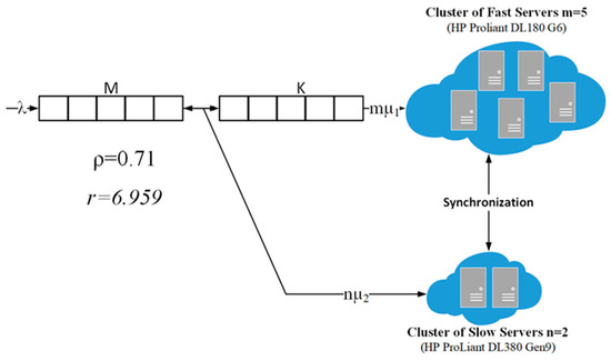
Figure 3.
Heterogeneous servers’ clusters with a stalling buffer.
Performance of servers’ W is calculated by using disks and disk arrays IOPS (input/output operations per second):
where —disk rotational speed per minute; —disc seek time in milliseconds; —disc latency in milliseconds. Disk array (RAID) IOPS is calculated as follows:
where Ndisks—the number of disks in an array; Drp—reading parity for disks array; Dwp—writing parity for disks array; DR%—total percent of reading; Dw%—total percent of writing; C—disks array overhead. Disk array RAID5 in slow and fast servers is used. For RAID5: Drp = 1, Dwp = 0, DR% = 70, Dw% = 30, C = 4.
Slow servers are HP Proliant DL180 G6 [36] width two Intel Xeon L5640@ 2.27 GHz processors (CPU Benchmarks 6358), with 128 GB DDR3 operating memory (read speed—13,887 MB/s; write speed—10,076 MB/s; MiNr/wspeed = 11,982, MiNtype = 8); we used five disks (Ndisks = 5) HP 3 TB 3.5” LFF 6 G Dual Port SAS 7.2 K RPM (MeXr/wdata = 97 Mb/s, data transferring rate MeXrate = 6.0 Gb/sec, IOPSdisk = 57) connected to RAID5 (IOPSraid = 18,098).
Fast servers are HP ProLiant DL380 Gen9 [37] width two Intel Xeon E5-2699 v4 @ 2.20 GHz processors (CPU Benchmarks 23200), with 128 GB DDR4 operating memory (read speed—22,075 MB/s; write speed—16,842 MB/s; MiNr/wspeed = 19,458.5, MiNtype = 16); we used seven disks (Ndisks = 7) HPE 2.4 TB SAS 12 G Enterprise 10 K LFF (MeXr/wdata = 195 Mb/s, data transferring rate MeXrate = 12 Gb/s, IOPSdisk = 133) connected to RAID5 (IOPSraid = 62843). Servers were divided into two synchronized clusters. The interarrival traffic time was distributed under the exponential law with parameter λ and the length of service was also distributed under this law with parameters µ1 and µ2. This was the case in systems using M length waiting buffer and K length stalling buffer (see Figure 3).
Performance of servers in clusters are calculated using the following formula (Figure 4):
where U—summarized performance processors of server controller (CPU Benchmarks); MeXrate—number of input output transferring’s to array of disks; MeXr/wdata—amount of data (bytes) transmitted per input/output operation; MiNr/wspeed—data transferring rate; MiNtype—coefficient taking into account the type of memory [38]. Calculated coefficient of performance for fast servers Wfast = 1190 and for slow server Wslow = 171.
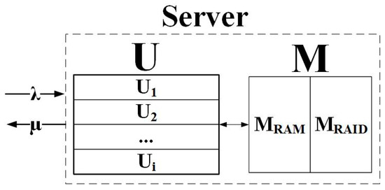
Figure 4.
Server components by queuing model.
The characteristics of the QS cluster with five fast and two slow servers are computed, and the results are displayed in Table 2.
Table 2.
Characteristics of the server’s cluster with stalling.
4.2. Modelling of Harvesters and Chainsaws Work Productivity
Coordination of technologies, processes, or devices with different capacities arises very often. Let us consider the problem of coordinated usage of harvesters (Timberjack 1270D) and chainsaws in spruce stands using data of comparative work productivity analysis [39]. Harvester (µ1) and chainsaw (µ2) work productivity have been compared in Table 3, taking into account the volume of the tree trunk.
Table 3.
Harvester and chainsaw work productivity comparison by volume of tree trunk [39].
Figure 5 shows how many harvesters and chainsaws will be needed for optimal systems work when the scope of forest harvesting is changed. We can see that, when using one harvester (m = 1) and a system load of 50 m3 for optimal systems work, 10 chainsaws are needed (Figure 5, graph on the left—see the yellow point on the graph and on the chainsaw axis is showing a 10, and on load axis we can see a 50). In contrast, when using two harvesters (m = 2) and a system load of 100 m3 for optimal systems work, 20 chainsaws will be needed (Figure 5, graph on the right—see the yellow point on the graph and on chainsaw axis is showing a 20, and on the load axis we can see a 100).
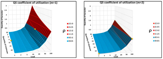
Figure 5.
The harvesters and chainsaws quantity dependence from forest harvesting scope.
5. Conclusions
In the paper, the model of stalling in a QS with heterogeneous channels and stalling buffer is presented, deriving the explicit probabilities of steady states using Chebyshev polynomials of the second order. The obtained expressions are numerically stable; their complexity does not depend on the number of states, and they provide a way of analytically studying QS characteristics. Moreover, the existence of a finite optimal size of the stalling buffer is proved and a numerical approach for the optimization of buffer size is developed.
The results showed that the appropriate choice of stalling buffer size provides assistance in solving the slow channel or server problem. The asymptotic conditions of optimal query distribution in channels when the ratio of the capacities of the fast and slow servers increases are also established. An application of the developed model in heterogeneous server clusters for work productivity modelling in the context of forest harvesting is also discussed herein.
This investigation of the developed model enables us to conclude that stalling is a universal solution that can be implemented into any heterogeneous system with any number of heterogeneous channels or servers.
Author Contributions
Conceptualization, L.S. and R.M.; methodology, L.S.; software, L.K.; validation, L.K. and R.M.; resources, L.K.; writing—original draft preparation, L.S. and L.K.; writing—review and editing, L.S., L.K. and R.M.; visualization, L.K.; supervision, L.S. All authors have read and agreed to the published version of the manuscript.
Funding
This research received no external funding.
Institutional Review Board Statement
Not applicable.
Informed Consent Statement
Not applicable.
Data Availability Statement
The data presented in this study are available in article.
Acknowledgments
We take an opportunity to kindly thank the anonymous reviewers for their valuable remarks.
Conflicts of Interest
The authors declare no conflicts of interest.
Appendix A
Proof of Lemma A1.
Let for enote At first, note the easily verifiable identity:
We can derive the relation between coefficients , whenever , Using the Equality (A1), the respective equations of steady-state probabilities in (1) and identities (3), we have
Established relationship and definition (3) imply the Lemma.□
Proof of Lemma A2.
Indeed, . Hence, according to (5),
After elementary steps by virtue of latter relationship and Lemma 1, one can make sure that
Proof of Theorem A1.
Let us consider Equation (1), for , or for , and assume that the waiting line is empty. Respectively, define, , and , . Then, according to (6), we have that
In addition, in virtue of Lemma 1,
Thus, (A2) and (A3) imply that relations among steady-state probabilities in (6) satisfy Equation (1), if , or , and the waiting line is empty.
Next, it is easy to see that Equation (7) is equivalent to recursive relation , which easily follow from respective Equation (1).
The expression of probability for state in which both channels and stalling buffer are only full, is derived after elementary manipulations using Equation (2) and following it remark, Newton binomial theorem and convinced that □
Proof of Lemma A3.
We can easily see that
Indeed, Lemma is true at . Now the relationship for , follows by virtue of respective equality of Lemma 1:
Proof of Theorem A2.
The expected number of queries in the QS by means of Lemma A3 is approximated as follows:
Then, differentiating it with respect to parameter K, equating the obtained derivative to zero and solving this equation, the approximate expression (i) of optimal stalling buffer size follows.
The approximate expression (ii) of optimal stalling buffer size is obtained in the same way using the expansion with the appropriated number of terms:
References
- Kleinrock, L. Queueing Systems, Volume 1: Theory; Wiley: New York, NY, USA, 2009. [Google Scholar]
- Larsen, R.L. Control of Multiple Exponential Servers with Application to Computer Systems. Ph.D. Thesis, University of Maryland at College Park, College Park, MD, USA, 1981. [Google Scholar]
- Rubinovitch, M. The slow server problem: A queue with stalling. J. Appl. Probab. 1985, 22, 879–892. [Google Scholar] [CrossRef]
- De Vericourt, F.; Zhou, Y.P. On the incomplete results for the heterogeneous server problem. Queueing Syst. 2006, 52, 189–191. [Google Scholar] [CrossRef]
- Goswami, V.; Samanta, S.K. Discrete-time bulk-service queue with two heterogeneous servers. Comput. Ind. Eng. 2009, 56, 1348–1356. [Google Scholar] [CrossRef]
- Rykov, V.V.E.; Efrosinin, D.V. On the slow server problem. Autom. Remote Control 2009, 70, 2013–2023. [Google Scholar] [CrossRef]
- Efrosinin, D.; Rykov, V. Heuristic solution for the optimal thresholds in a controllable multi-server heterogeneous queueing system without preemption. In Proceedings of the International Conference on Distributed Computer and Communication Networks, Moscow, Russia, 19–22 October 2015; pp. 238–252. [Google Scholar]
- Shi, C.; Li, Y.; Zhang, J.; Sun, Y.; Philip, S.Y. A survey of heterogeneous information network analysis. IEEE Trans. Knowl. Data Eng. 2017, 29, 17–37. [Google Scholar] [CrossRef]
- Kaklauskas, L.; Sakalauskas, L.; Denisovas, V. Stalling for solving slow server problem. RAIRO Oper. Res. 2019, 53, 1097–1107. [Google Scholar] [CrossRef]
- Kalyanaraman, R.; Hellen, A. M/M/2 Heterogeneous Server Queue with Variant Breakdown and with Discouraged Arrivals. Math. Stat. Eng. Appl. 2022, 71, 1447–1458. [Google Scholar]
- Kalyanaraman, R.; Hellen, A. A Two Heterogeneous Server Queue with Variant Breakdown and with Discouraged Arrivals, Balking. Neuro Quantol. 2022, 20, 4142. [Google Scholar]
- Elsayed, E.A. Multichannel queueing systems with ordered entry and finite source. Comput. Oper. Res. 1983, 10, 213–222. [Google Scholar] [CrossRef]
- Rana, P.S. A discrete time queueing problem with S heterogeneous groups of channels. Microelectron. Reliab. 1985, 25, 455–459. [Google Scholar]
- Rana, P.S. A queueing problem with random memory arrivals and heterogeneous servers. Microelectron. Reliab. 1985, 25, 645–650. [Google Scholar]
- Rosberg, Z.; Makowski, A.M. Optimal routing to parallel heterogeneous servers-small arrival rates. IEEE Trans. Autom. Control 1990, 35, 789–796. [Google Scholar] [CrossRef][Green Version]
- El-Taha, M.; Stidham, S., Jr. Deterministic analysis of queueing systems with heterogeneous servers. Theor. Comput. Sci. 1992, 106, 243–264. [Google Scholar] [CrossRef][Green Version]
- Chirkova, J.; Mazalov, V.; Morozov, E. Equilibrium in a queueing system with retrials. Mathematics 2022, 10, 428. [Google Scholar] [CrossRef]
- Cabral, F.B. The slow server problem for uninformed customers. Queueing Syst. 2005, 50, 353–370. [Google Scholar] [CrossRef]
- Rykov, V.V. Monotone control of queueing systems with heterogeneous servers. Queueing Syst. 2001, 37, 391–403. [Google Scholar] [CrossRef]
- Efrosinin, D.; Sztrik, J. Performance analysis of a two-server heterogeneous retrial queue with threshold policy. Qual. Technol. Quant. Manag. 2011, 8, 211–236. [Google Scholar] [CrossRef]
- Efrosinin, D.; Sztrik, J. Optimal control of a two-server heterogeneous queueing system with breakdowns and constant retrials. In Proceedings of the International Conference on Information Technologies and Mathematical Modelling, Katun, Russia, 12–16 September 2016; pp. 57–72. [Google Scholar]
- Pankratova, E.; Moiseeva, S.; Farkhadov, M. Infinite-Server Resource Queueing Systems with Different Types of Markov-Modulated Poisson Process and Renewal Arrivals. Mathematics 2022, 10, 2962. [Google Scholar] [CrossRef]
- Dudin, A.; Dudina, O.; Dudin, S.; Gaidamaka, Y. Self-service system with rating dependent arrivals. Mathematics 2022, 10, 297. [Google Scholar] [CrossRef]
- Efrosinin, D.; Stepanova, N. Estimation of the optimal threshold policy in a queue with heterogeneous servers using a heuristic solution and artificial neural networks. Mathematics 2021, 9, 1267. [Google Scholar] [CrossRef]
- Efrosinin, D.; Stepanova, N.; Sztrik, J. Algorithmic analysis of finite-source multi-server heterogeneous queueing systems. Mathematics 2021, 9, 2624. [Google Scholar] [CrossRef]
- Hetherington, T.H.; Rogers, T.G.; Hsu, L.; O’Connor, M.; Aamodt, T.M. Characterizing and evaluating a key-value store application on heterogeneous CPU-GPU systems. In Proceedings of the IEEE International Symposium on Performance Analysis of Systems and Software (ISPASS), New Brunswick, NJ, USA, 1–3 April 2012; pp. 88–98. [Google Scholar]
- Ciznicki, M.; Kierzynka, M.; Kopta, P.; Kurowski, K.; Gepner, P. Benchmarking JPEG 2000 implementations on modern CPU and GPU architectures. J. Comput. Sci. 2014, 5, 90–98. [Google Scholar] [CrossRef]
- Kadjo, D.; Ayoub, R.; Kishinevsky, M.; Gratz, P.V. A control-theoretic approach for energy efficient CPU-GPU subsystem in mobile platforms. In Proceedings of the 52nd Annual Design Automation Conference, San Francisco, CA, USA, 8–12 June 2015; p. 62. [Google Scholar]
- Choi, W.; Duraisamy, K.; Kim, R.G.; Doppa, J.R.; Pande, P.P.; Marculescu, D.; Marculescu, R. On-Chip Communication Network for Efficient Training of Deep Convolutional Networks on Heterogeneous Manycore Systems. IEEE Trans. Comput. 2018, 67, 672–686. [Google Scholar] [CrossRef]
- Almusaddar, G.; Naghibijouybari, H. Exploiting Parallel Memory Write Requests for Covert Channel Attacks in Integrated CPU-GPU Systems. arXiv 2023, arXiv:2307.16123. [Google Scholar]
- Jin, X.; Min, G. Analytical queue length distributions of GPS systems with long range dependent service capacity. Simul. Model. Pract. Theory 2009, 17, 1500–1510. [Google Scholar] [CrossRef]
- Lu, J.; Ma, M. Cross-layer QoS support framework and holistic opportunistic scheduling for QoS in single carrier WiMAX system. J. Netw. Comput. Appl. 2011, 34, 765–773. [Google Scholar] [CrossRef]
- Okorogu, V.N.; Okafor, C.S. Improving Traffic Management in a Data Switched Network Using an Adaptive Discrete Time Markov Modulated Poisson Process. Eur. J. Sci. Innov. Technol. 2023, 3, 542–562. [Google Scholar]
- Hruby, T.; Bos, H.; Tanenbaum, A.S. When Slower Is Faster: On Heterogeneous Multicores for Reliable Systems. In Proceedings of the USENIX Annual Technical Conference, San Jose, CA, USA, 26–28 June 2013; pp. 255–266. [Google Scholar]
- Wang, J.; Zhang, Q.; Rong, H.; Xu, G.H.; Kim, M. Leveraging Hardware Probes and Optimizations for Accelerating Fuzz Testing of Heterogeneous Applications. In Proceedings of the 31st ACM Joint European Software Engineering Conference and Symposium on the Foundations of Software Engineering, San Jose, CA, USA, 3–9 November 2023; pp. 1101–1113. [Google Scholar]
- Hewlet Packard Enterprice. HPE ProLiant DL380 Gen9 Server. 2019. Available online: https://h20195.www2.hpe.com/v2/getpdf.aspx/c04346247.pdf (accessed on 15 November 2022).
- Hewlet Packard Enterprice Support Center. HPE ProLiant DL180 G6 Server—Overview. 2019. Available online: https://support.hpe.com/hpsc/doc/public/display?docId=emr_na-c01709693 (accessed on 15 November 2022).
- Kovalenko, S.M.; Kazancceva, L.V.; Supronenko, D.V. Integrated Indicator of the Performance of Servers. The Online Scientific and Methodological Journal “Herald of MSTU MIREA”. 2014. Available online: https://rtj.mirea.ru/upload/medialibrary/3df/10-kovalenko_kazantsev.pdf (accessed on 15 November 2022).
- Mizaras, S.; Kombaris, N. Economic assessment of multifunctional forests in conservation land areas of Varniai regional park. Agric. Sci. 2012, 19, 98–105. [Google Scholar]
Disclaimer/Publisher’s Note: The statements, opinions and data contained in all publications are solely those of the individual author(s) and contributor(s) and not of MDPI and/or the editor(s). MDPI and/or the editor(s) disclaim responsibility for any injury to people or property resulting from any ideas, methods, instructions or products referred to in the content. |
© 2024 by the authors. Licensee MDPI, Basel, Switzerland. This article is an open access article distributed under the terms and conditions of the Creative Commons Attribution (CC BY) license (https://creativecommons.org/licenses/by/4.0/).