Transfer Learning-Based Remaining Useful Life Prediction Method for Lithium-Ion Batteries Considering Individual Differences

Abstract

With the wide utilization of lithium-ion batteries in the fields of electronic devices, electric vehicles, aviation, and aerospace, the prediction of remaining useful life (RUL) for lithium batteries is important. Considering the influence of the environment and manufacturing process, the degradation features differ between the historical batteries and the target ones, and such differences are called individual differences. Currently, lithium battery RUL prediction methods generally use the characteristics of a large group of historical samples to represent the target battery. However, these methods may be vulnerable to individual differences between historical batteries and target ones, which leads to poor accuracy. In order to solve the issue, this paper proposes a prediction method based on transfer learning that fully takes individual differences into consideration. It utilizes an extreme learning machine (ELM) twice. In the first stage, the relationship between the capacity degradation rate and the remaining capacity is constructed by an ELM to obtain the adjusting factor. Then, an ELM-based transfer learning method is used to establish the connection between the remaining capacity and the RUL. Finally, the prediction result is adjusted by the adjusting factor obtained in the first stage. Compared with existing typical data-driven models, the proposed method has better accuracy and efficiency.

1. Introduction

With the widespread application and technological advancement, lithium batteries have become important components in the fields of electronic devices, electric vehicles, aviation, and aerospace [1,2]. Although lithium batteries have advantages, such as high energy density, a wide operating temperature range, and high charging efficiency [3], the degradation of the remaining capacity for lithium batteries may accelerate the aging of connected batteries, reduce the endurance of devices, influence the security, and may cause loss of property [4,5]. In order to determine the possible remaining usage time for batteries before their remaining capacity reaches the failure threshold so that they can be replaced in time, the prediction of the remaining useful life (RUL) for lithium batteries is essential [6,7,8].

At present, RUL prediction is generally faced with the difficulty that the historical data used to construct battery prediction models often exhibit inherent stochastic biases compared to operational battery data, resulting in substantial uncertainties within the established predictive models. Consequently, accurately evaluating the RUL prediction of lithium batteries has become a challenging endeavor within the current landscape of lithium battery health assessment. In the field of lithium battery remaining lifespan prediction, experts and scholars from various countries have made substantial contributions. Currently, there are two main categories of methods: those based on physical models [9,10] and those based on data-driven approaches [1,2,7].

For physical model-based prediction methods, the methods based on physical models establish battery aging models by analyzing internal physical or chemical changes. Steven [4] discussed the limitations of predicting specific discharge capacities, proposing a paradigm shift toward excellence in data-driven approaches within the realm of materials research. Gao [11] introduced the estimation of battery capacity using measurable parameters during battery discharge cycles that effectively prevent the continued use of batteries beyond their service life threshold, thereby mitigating a range of safety concerns. Osama [12] presented a novel framework incorporating a deep neural network with memory features, achieving a balance between accuracy and computational complexity. However, due to the inherent complexity of internal reactions within batteries and the significant variations in the aging processes among different types of batteries, models constructed using this approach are generally applicable to a specific type and set of operating conditions of batteries.

On the other hand, data-driven methods utilize historical operational data of batteries to construct aging prediction models. As these methods do not require a precise understanding of the exact physical and chemical mechanism parameters, leading to battery failure, they can directly uncover patterns of lithium battery performance degradation from electrical parameters, such as voltage and current. Consequently, this approach is more versatile and has gradually emerged as the predominant method for predicting the remaining lifespan of lithium batteries in various contexts in recent years. Gao [13] proposed a novel Multi-Kernel Support Vector Machine (MSVM) based on multiple kernel functions (polynomial and radial basis kernel functions) and utilized a particle swarm optimization algorithm to search for MSVM model parameters, penalty factors, and weight coefficients. This approach effectively addresses issues related to the weak generalization of SVM and data transfer. Zhang [14] introduced a bidirectional long short-term memory (Bi-LSTM) network, dropout technique, and Bayesian variational inference to quantify the uncertainty in RUL prediction results. This method provides 95% confidence intervals and probability density functions (PDFs) for RUL prediction results, effectively addressing the problem of insufficiently considering the lifespan information contained in multiple internal states of lithium-ion batteries. Ren [15] proposed a deep learning approach that combines autoencoders with deep neural networks (DNNs) to extract multidimensional RUL information, enhancing prediction accuracy. Ansari [16] presented an RUL prediction method based on Multi-Channel Input (MCI) configuration and Recurrent Neural Network (RNN) algorithms, including both Single-Channel Input (SCI) and MCI configurations. Compared to the single channel-based method, this method significantly reduces prediction errors. Tang [17] introduced a hybrid RUL prediction model based on Complete Ensemble Empirical Mode Decomposition with Adaptive Noise (CEEMDAN) and a bi-directional gated recurrent unit, along with genetic algorithm-based factor improvement and dynamic population weighting to accelerate algorithm convergence. Danniel [18] proposed a deep learning-based method trained on the widely used Oxford battery degradation dataset, utilizing Generative Adversarial Networks (GANs). The network architecture adopted long short-term memory (LSTM), hierarchical strategies, and custom loss functions, achieving accurate predictions for small-sample condition RUL.

The above data-driven methods directly leverage historical sample data from lithium batteries to predict future aging trends by establishing statistical or machine learning models. These methods circumvent the need for intricate mathematical or physical modeling processes, significantly enhancing the generality of lithium battery lifespan prediction models. However, due to the differences in the manufacturing process, environmental factors, and the uncertainty during the degradation process, the difference between the degradation characteristics of different batteries (individual differences) may be great. Within the process of constructing predictive models using a set of historical samples, such approaches often fail to adequately account for individual differences. As a result, predictive models developed using the overall sample data struggle to accurately reflect the aging trends of in-service batteries, leading to the accumulation of predictive bias [19,20].

In order to reduce the error caused by individual differences, this paper introduced a new proposed method. First, calculate the degradation rate of historical capacity data and target battery capacity data, and then use an extreme learning machine (ELM) to construct the relationship between the capacity degradation rate and the capacity of historical data and use the trained model on the target battery’s existing degradation rate to predict the capacity data. After that, the adjusting factor can be obtained according to the differences in capacity obtained by ELM and the real capacity data. Finally, another transfer learning-based ELM is applied to predict the RUL according to the capacity data, and the adjusting factor is used to adjust the prediction result.

The contributions of the method are as follows:

• Using the ELM model can reduce the required training time because compared with traditional neural networks, ELM does not need to follow a critical gradient descent process;
• The proposed ELM-based transfer learning method can improve the stability of the traditional ELM method, reducing error caused by the inherent features of the ELM model in which the initial parameters are arbitrarily generated;
• The adjusting factor can further enhance the precision and accuracy of RUL prediction by clearly identifying and evaluating individual differences.

In general, compared with existing prediction models, our method has better performance in accuracy and efficiency.

The remainder of this paper is organized as follows. Section 2 presents the procedure of the proposed method, Section 3 introduces the case study and experiment result, Section 4 gives the discussion, and finally, the conclusions are illustrated in Section 5.

2. Proposed Method

A flowchart of the proposed model for RUL prediction is shown in Figure 1. The entire approach consists of three parts: data pre-processing with ELM model construction, adjusting factor gain, and transfer learning-based RUL prediction.

(1)

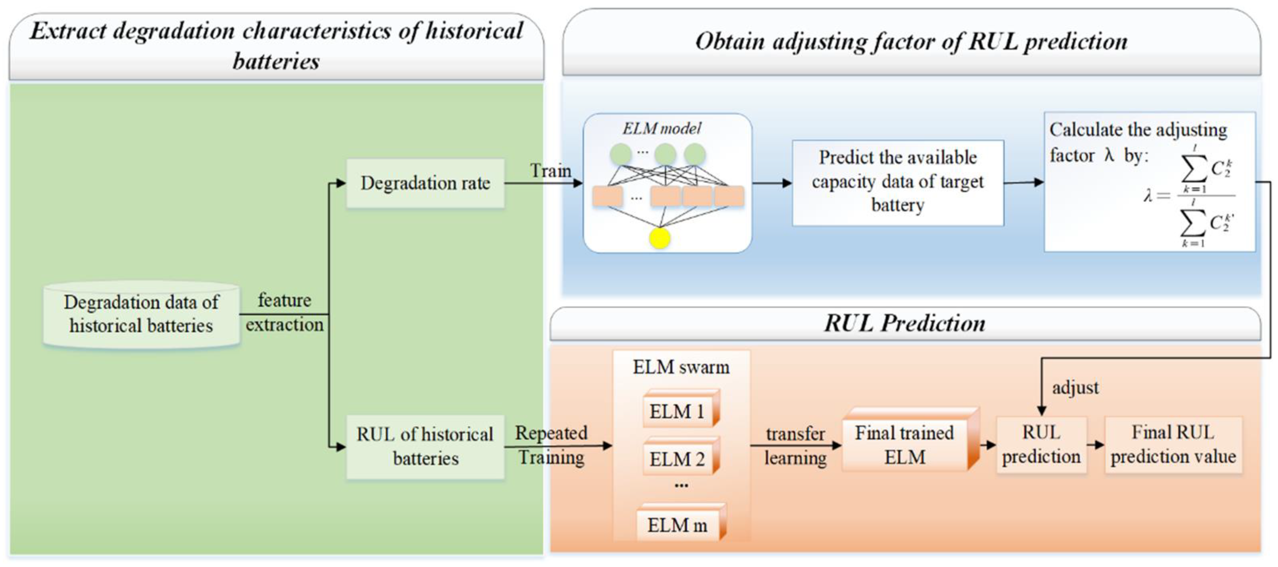
Data pre-processing with ELM model construction: The degradation rate data are calculated from the original remaining capacity data. Then, the beginning and ending points are marked on the capacity data of the historical group. After that, a typical three-layer ELM is used to construct the relationship between the degradation rate obtained in data pre-processing and the remaining capacity of historical data;

(2)

Adjusting factor gain: The ELM model constructed in step (1) is utilized on the known part of degradation rate data for the target group. The output remaining capacity is compared with the real remaining capacity data of the target battery, and the adjusting factor is calculated according to their differences;

(3)

Transfer learning-based RUL prediction: Several ELMs are used to construct the relationship between the remaining capacity and RUL of historical data. They share different weights according to their performance, which helps with the construction of the final ELM model. The final ELM is applied to the data of the target battery to predict the RUL. Then, the result is adjusted by the adjusting factor obtained in step (2) and then becomes the final prediction results of the RUL.

2.1. Data Pre-Processing

In this section, we use the capacity data provided by Severson et al. [21] to show the procedure of our model. The RUL of historical batteries is obtained by accelerated aging experiments. The lithium batteries are cycled to failure under fast-charging conditions. These lithium-ion batteries (LIBs) were tested in Arbin LBT potentiostat at 30 °C, and they all have a nominal capacity of 1.1 Ah. The dataset consists of 124 commercial lithium-ion batteries with lithium-ion phosphate (LFP)/graphite cells manufactured by A123 Systems (APR18650M1A). The charging policy of these LIBs has the format “C1(Q1)-C2”, where C1 and C2 are the first and second (constant current) CC charging steps, respectively, and Q1 is the state-of-charge (SOC, %) when the currents switch. The charging parameters of these batteries are shown in

Table 1. Charging policies of LIBs from Severson et al.

	C1	Q1	C2
Case 1	6C	40%	3C
Case 2	5.3C	54%	4C
Case 3	5.9C	60%	3.1C
Case 4	5.6C	36%	4.3C

[21]. The paper has provided 124 groups of datasets. However, due to the limitation of article length, we provide the experiment result of 6 groups of data that have the most obvious individual differences so that they can demonstrate our method’s outstanding performance in dealing with individual differences.

The data of the capacity of case 1 to case 4 are shown in Figure 2, Figure 3, Figure 4 and Figure 5.

Although the manufacturing process, the materials, and the charging policy are identical according to Table 1, we can clearly observe in Figure 2, Figure 3, Figure 4 and Figure 5 that the maximum capacity, the degradation rate, the changing trend of degradation rate, and the failure time are different. All the above differences can be concluded as individual differences.

After obtaining the capacity data, the degradation rate of the batteries is calculated from the capacity data. Assume the capacity data for the historical sample and the target battery are, respectively, expressed as [$C_1^i$] (i = 1, 2, 3…) and [$C_2^i$] (i = 1, 2, 3…). The degradation rate can be expressed as:

$$D_{r1}=\frac{C_1^i-C_1^{i+1}}{C_1^{i+1}}, D_{r2}=\frac{C_2^i-C_2^{i+1}}{C_2^{i+1}}$$

(1)

where $D_{r1}$ is the degradation rate of the historical sample and $D_{r2}$ is the degradation rate of the target battery.

Repeat the calculation in Formula (1) and obtain the degradation rate of all corresponding points. Then, the RUL of historical batteries and the degradation rate of both historical and target batteries are extracted.

2.2. Obtaining the Adjusting Factor for RUL Prediction

There are three parts to this section. First, the construction of an extreme learning machine (ELM) that finds the relationship between the degradation rate of historical data and introduces capacity of the historical data. Then, the trained ELM model is used to predict the capacity of the target battery. Finally, the predicted capacity of the target battery is used to obtain the adjusting factor.

2.2.1. The Construction of the ELM

In this paper, an extreme learning machine (ELM) is used to construct the relationship between the degradation rate data and capacity data in Section 2.2 for the first time, as well as the relationship between the capacity data and the RUL in Section 2.3 for the second time. In the experiment section, the hyper-parameter for the ELM is 10 nodes at the input layer, 7 nodes at the hidden layer, and 1 node at the output layer. The values of the hyper-parameter are determined according to stability and efficiency examined in pre-experiments and historical experiences.

Construct a single hidden-layer extreme learning machine (ELM) network. Suppose the capacity of the battery sample can be expressed as ($X_i$, $t_i$) and $X_i$= [$x_{i,m}$] (m = 1, 2, 3…), $Y_i$= [$y_{i,m}$] (m = 1, 2, 3…), where $i$ represents the $i$th battery, $X_i$ is the input to the network, and $Y_i$ is the output of the network:

$${\sum }_{i=1}^{length}{\beta }_{i}g(W_i·X_j+b_i)=O_j, j=1,2,3,\dots \mathrm{N}$$

(2)

where $W_i$ is the input weight matrix,${\beta }_i$ is the output weight matrix, $b_i$ is the bias matrix, $g$(x) is the activate function where the sigmoid function is used, $O_j$ is the output, and N is the total quantity.

To minimize the error, there should be:

$${\sum }_{j=1}^N{|O}_j-y_j|=0$$

(3)

which means there exist ${\beta }_i$, $W_i$, and $b_i$, such that:

$${\sum }_{i=1}^{length}{\beta }_{i}g(W_i·X_j+b_i)=y_j$$

(4)

The complex form according to the formula is:

$$H={\left[\begin{array}{ccc}g(w_{\mathrm{1,1}}^T{X}_1-{\theta }_1)& \cdots & g(w_{N,1}^T{X}_1-{\theta }_N)\\ ⋮& \ddots & ⋮\\ g(w_{1,D}^T{X}_D-{\theta }_1)& \cdots & g(w_{N,D}^T{X}_D-{\theta }_N)\end{array}\right]}_{D\times N}$$

where the other two parameters are the following, respectively:

$$\beta ={\left[\begin{array}{c}{\beta }_1^T\\ ⋮\\ {\beta }_N^T\end{array}\right]}_{N\times n}Y={\left[\begin{array}{c}{Y}_1^T\\ ⋮\\ Y_D^T\end{array}\right]}_{D\times n}$$

where H is the output at the hidden layer nodes and Y is the expected output.

In order to minimize the error, the mission can be turned into minimizing:

$$\left|\right(W_i, b_i) {\beta }_i-Y| i=1, 2, 3, \dots$$

(5)

which is identical to minimizing the loss function:

$$\mathrm{L}={\sum }_{j=1}^N[{\sum }_{i=1}^{length}{{\beta }_{i}g(W}_i·X_j+b_i)-y_j{]}^2$$

(6)

Compared with other traditional gradient-degradation methods, such as backpropagation (BP), the advantage of the ELM is that once $W_i$ and $b_i$ are chosen arbitrarily, training the neural network can be turned into solving a first-order linear task, which is more efficient.

Suppose the step width of the historical data trained is l.

The output of the network can be expressed as:

$$H(W_1,\dots W_L,b_1,\dots ,b_L,X_1,\dots ,X_N)=\left[\begin{array}{ccc}g\left(W_1·X_1+b_1\right)& \cdots & g\left(W_L·X_1+b_L\right)\\ ⋮& \ddots & ⋮\\ g\left(W_1·X_N+b_1\right)& \cdots & g\left(W_L·X_N+b_L\right)\end{array}\right]$$

(7)

Thus, the purpose is to minimize:

$$\mathrm{E}={\sum }_{j=1}^N[{\sum }_{i=1}^L{\beta }_i g(W_i·X_j+b_i)-t_j{]}^2$$

(8)

2.2.2. Adjusting Factor

In this section, the trained ELM is used to predict the capacity data of the target battery. Then, the predicted capacity data are compared with the real capacity data; thus, the adjusting factor based on the differences between the predicted capacity data and real capacity data can be obtained.

Assume the capacity of the $ith$ battery samples for training is $C_{train}$ = [$c_m^i$] (m = 1, 2, 3…). The available capacity of the target battery is $C_{pre}$ = [$c_{pre,j}^{ }$] (j = 1, 2, 3…). The capacity degradation rate of the battery samples $L_{train}$ = [$l_m^i$] (i = 1, 2, 3…, m = 1, 2, 3…) for training can be expressed as:

$$l_m^i=[\frac{c_m^{i-1}-c_m^i}{c_m^{i-1}}] i=1,2,3,\dots$$

(9)

The capacity degradation rate of the target battery $L_{pre}$= [$l_{pre,j}$] (i = 1, 2, 3…) can be expressed as:

$$l_{pre,j}=[\frac{c_{pre,j-1}^{ }-c_{pre,j}^{ }}{c_{pre,j-1}^{ }}] j=1,2,3,\dots$$

(10)

After obtaining the capacity data and calculating the degradation rate data, train an ELM network to construct the relationship between the capacity and the degradation rate. Suppose the quantity of the input nodes of the ELM is q, and the output node is one. At time point t, the input nodes consist of q capacity data [$c_m^{t-q+1},c_m^{t-q+2},\dots ,c_m^{t-1},c_m^t$], which are the capacity value at the moment and q−1 numbers of data before it. The output nodes are the degradation rate at the moment [$l_m^t$].

After training an ELM neural network, we use the steps shown in this section. Suppose the quantity of the input nodes of the ELM is q. Then, use the first existing q degradation rate [$l_{pre,j}$] (j = 1, 2, 3 …q) to make a multi-step prediction.

The steps of multi-step prediction are shown in Figure 6. The output of the prediction is actually the predicted value for the next time point. Then, integrate the new value into the sequence, place it at the bottom of the sequence to generate the new sequence, and use the new sequence to continue to make the prediction.

First, input the q degradation rate data of the target battery into the trained ELM network to obtain the predicted (q + 1)th capacity data. Then, the predicted capacity data are used to generate the (q + 1)th degradation rate. In the next prediction step, the obtained (q + 1)th degradation rate data will be input into the ELM network again to obtain the (q + 2)th predicted data. Repeat the above steps until the predicted value reaches the failure threshold of the target battery. The predicted capacity data of the target battery is $C_{pre}^{\prime }$ = [$c_{pre,j}^{\prime }$] (j = 1, 2, 3…).

Based on the predicted capacity data $C_{pre}^{\prime }$ and the real capacity data $C_{pre}$ of the target battery, the adjusting factor λ can be calculated based on the consequence above:

$$\mathsf{\lambda }=\frac{{\sum }_{k=1}^l{C}_{pre}^k}{{\sum }_{k=1}^l{C}_{pre}^{k\prime }}$$

(11)

2.3. RUL Prediction

In this section, an ELM-based transfer learning method is used to construct the relationship between the capacity and the RUL of the historical data. It combines the ELM model with transfer learning because of the inherent feature that the weight and bias of the ELM are arbitrary, which makes the performance of ELM unstable. Then, the ELM-based transfer learning method is used to predict the RUL of the target battery, and the prediction results are adjusted by the adjusting factor obtained in Section 2.2.

2.3.1. ELM-Based Transfer Learning

Due to its fast training speed and high prediction accuracy, the ELM network has been widely used in the field of remaining life prediction of lithium batteries. However, due to the randomness of the initial values of ELM network parameters, the predictive performance of ELM networks trained with the same degradation samples of lithium batteries is often different. Therefore, we propose a transfer learning model based on an ELM network to overcome the shortcomings of traditional ELM networks and further improve the prediction accuracy of the proposed model.

As shown in Figure 1, after we obtained the capacity degradation data of historical batteries, the ELM model was repeatedly trained, and m-trained ELM neural networks were obtained. We define these trained ELM neural networks as the ELM swarm (ELMS). Assuming that the number of input nodes of each ELM in the ELMS is n, the first n field capacity degradation data of the target battery are selected and input into each trained ELM, and the multi-step prediction method shown in the figure is adopted to obtain the capacity prediction sequence of each trained ELM network. Calculate the mean absolute error (MAE) between the capacity prediction sequence for each ELM network and the actual capacity degradation data for the target cell:

$${MAE}_i=\frac{\sum _{j=1}^k|C_{i,j}^{predict}-C_j|}{k}$$

(12)

where ${MAE}_i(i=\mathrm{1,2},\dots ,m)$ represents the prediction result of the $i^{th}$ ELM network; $C_{i,j}^{predict}$ represents the $i^{th}$ capacity prediction value obtained by the $i^{th}$ trained ELM network; $C_j$ represents the $j^{th}$ actual capacity degradation data of the target cell; and k represents the amount of field capacity degradation data for the target battery. The smaller the MAE, the better the ELM can fit the existing capacity data of the target battery.

Based on the MAE of all trained ELM networks, the transfer weight, ${weight}_i(i=\mathrm{1,2},\dots m)$, corresponding to the $i^{th}$ ELM network is obtained using the following formula:

$${weight}_i=\frac{{MAE}^{max}-{MAE}_i}{{MAE}^{max}-{MAE}^{min}}$$

(13)

where ${MAE}^{max}$ represents the maximum value of MAE and ${MAE}^{min}$ represents the minimum value of MAE.

Then, the RUL predicted value of the target battery by the $i^{th}$ trained ELM network ${RUL}_i(i=\mathrm{1,2},\dots m)$ is obtained by a multi-step prediction method. Based on the transfer weights obtained above, the final RUL predicted value ${RUL}_{final}$ is calculated:

$${RUL}_{final}={\sum }_{i=1}^m{weight}_i\times {RUL}_i$$

(14)

2.3.2. Adjusting the Results

Due to the accumulation effect of error, when the prediction process is near the breakdown threshold, there are only a small number of points. Thus, the error caused by individual differences is relatively low. By contrast, at the beginning of the prediction, since there are many points followed, the error caused by individual differences is relatively high. In this case, we proposed an adaptive adjusting method based on the adjusting factor $\mathsf{\lambda }$. The result ${RUL}_{final}$ obtained in Section 2.3.1 can be expressed as ${RUL}_{final}$ = [${rul}_j$] (j = 1, 2, …, n), where n is the total number of predicted points. The adjusted RUL is:

$${rul}_{adjust,j}={{\mathsf{\lambda }}^{10}rul}_j (j=1,2,\dots ,n-100)$$

$${rul}_{adjust,j}={\mathsf{\lambda }}^{0.1(n-j)}{rul}_j (j=n-99, ,n-98, \dots ,n)$$

where n is the total number of points that we use our method to make the prediction and $\mathsf{\lambda }$ is the adjusting factor obtained in Section 2.2.2. Thus, the adjusted result is ${RUL}_{adjust}$ = ${[rul}_{adjust,j}]$(j = 1, 2, …, n).

3. Case Study

In this section, we use examples to verify the performance of the proposed method. We apply our prediction model to the open-source capacity data provided by Severson et al. [21], and these capacity data are shown in Figure 2, Figure 3, Figure 4 and Figure 5. The practical applicability of the dataset has been proved in [22,23,24]. All of these batteries were tested on the battery-accelerated life experiment platform. The related experiment condition has been shown in Section 2.1.

According to [25,26,27], a battery is regarded as under the threat of failure when its capacity reaches 95% of its maximum capacity. Therefore, we set the threshold for the beginning of the prediction at the time point when the remaining capacity reaches 95% of the maximum capacity. In other words, once the battery has degraded 5% of its maximum capacity, the prediction process starts. Also, a battery is regarded as a failure when its capacity reaches 80–90% of its maximum capacity. Therefore, we set the failure threshold at 0.89 mAh, which is about 85% of the starting capacity value of the four cases shown in Figure 2, Figure 3, Figure 4 and Figure 5. Thus, the prediction ends at the time when the capacity reaches 0.89 mAh. The historical battery and the target battery of each case are defined in

Table 2. Case condition.

		Historical Battery	Target Battery
Case 1	Case 1-1	Battery 1	Battery 2
	Case 1-2	Battery 2	Battery 1
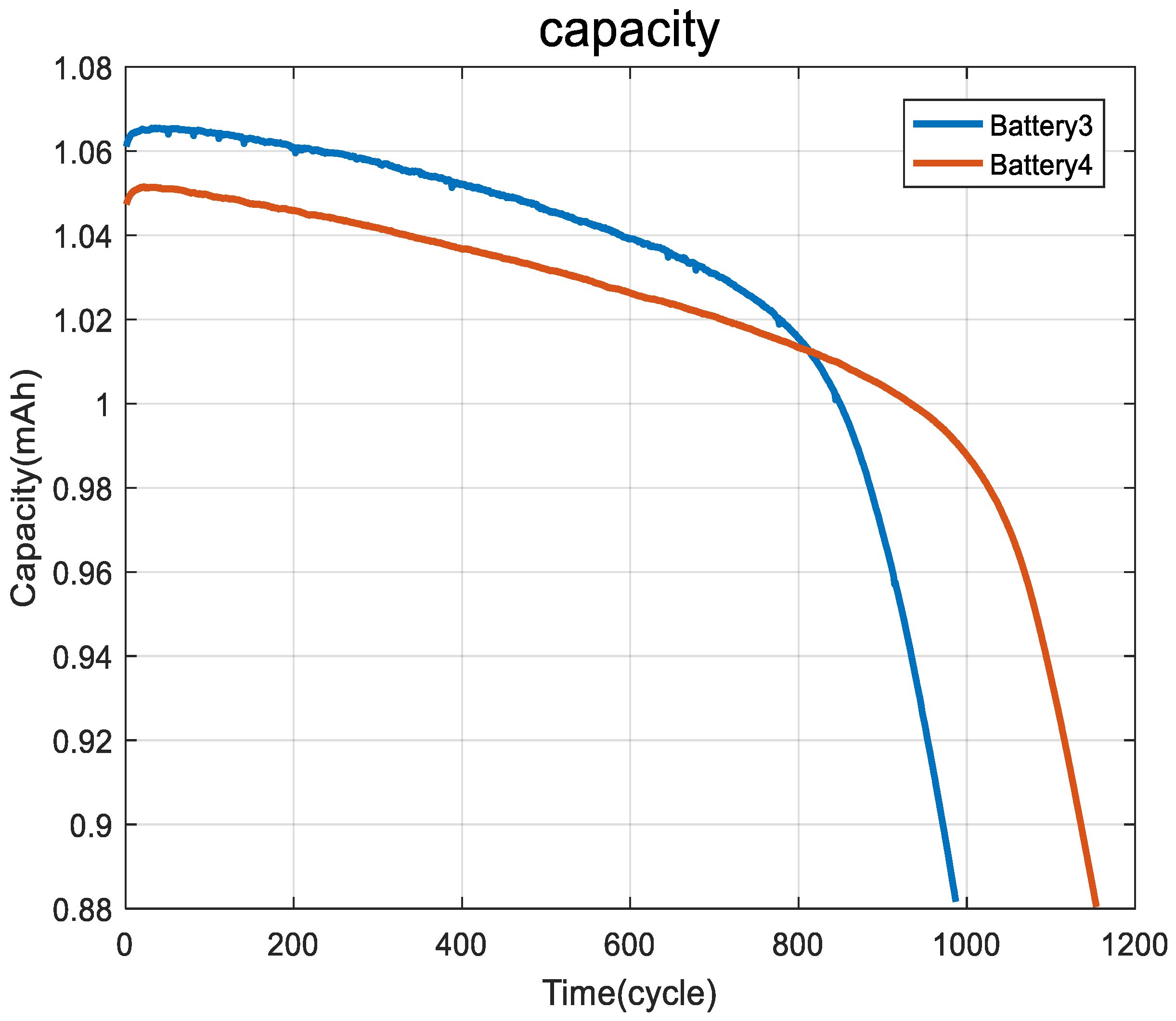
Case 2	Case 2-1	Battery 3	Battery 4
	Case 2-2	Battery 4	Battery 3
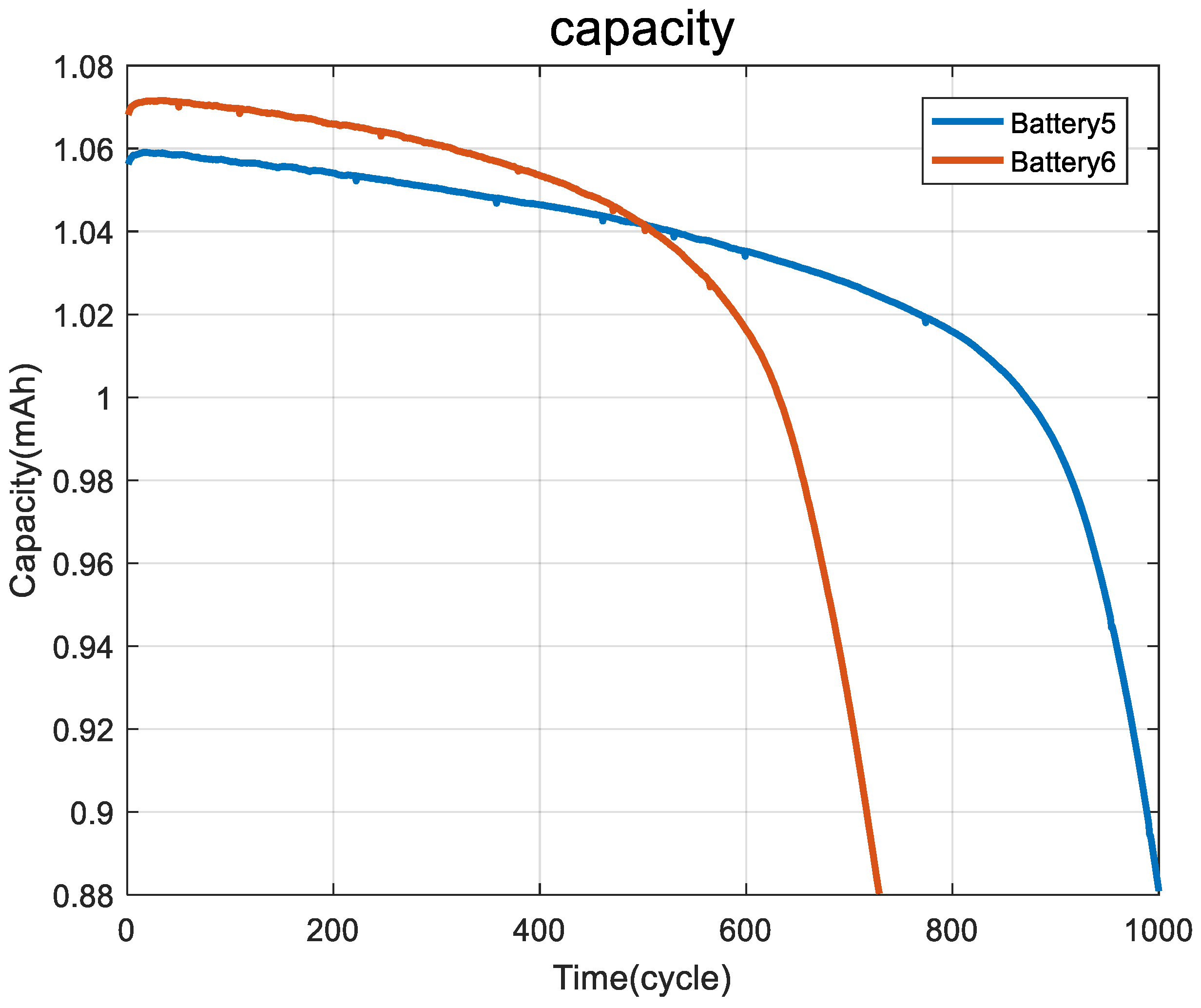
Case 3	Case 3-1	Battery 5	Battery 6
	Case 3-2	Battery 6	Battery 5
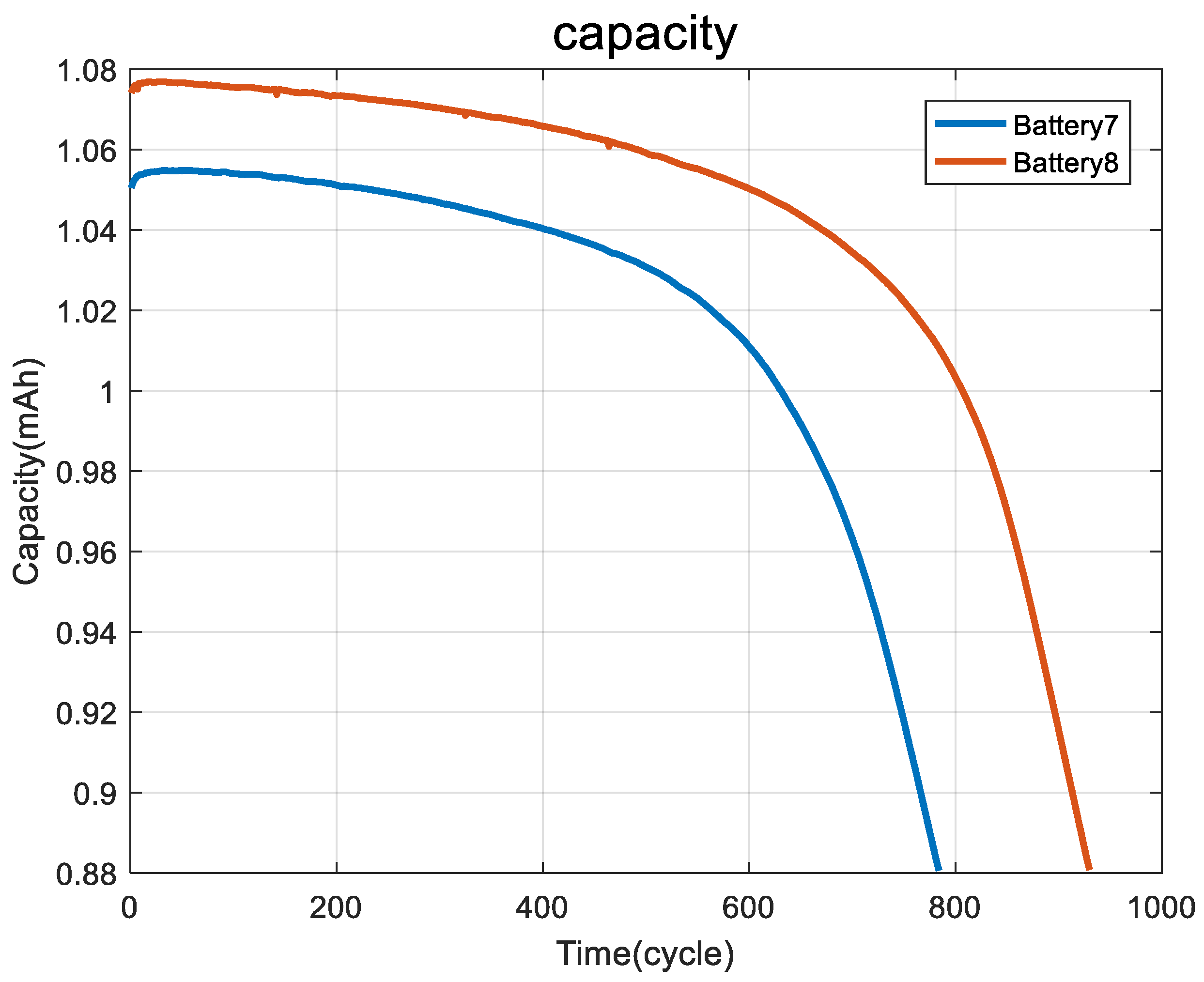
Case 4	Case 4-1	Battery 7	Battery 8
	Case 4-2	Battery 8	Battery 7

.

In each case shown in Table 2, there are two batteries, and thus there are two capacity degradation curves. We use one of them as the historical battery and another one as the target battery to make the prediction. Then, we reverse their characters and make another prediction.

To show the superiority of the proposed model, we conducted some comparison experiments. We first compared the results of our method with a prediction method that only used the ELM to construct the relationship between capacity data and the RUL. The settings of the ELM are ten input layers, seven hidden layers, and one output layer. Then, we used our proposed method with the same layer setting to make the prediction on the same data. Finally, we compared the performance of our method to hybrid transfer learning (HTL) [28] proposed by Ma and long short-term memory neural networks (LSTs) [29] presented by Zhou. These two published papers used the same datasets.

The RUL prediction results of the proposed method (PM) and the other four methods are shown in Figure 7, Figure 8, Figure 9, Figure 10, Figure 11, Figure 12, Figure 13 and Figure 14, and the numerical results for the mean average percentage error (MAPE) are shown in

Table 3. Comparison of errors.

Case Number	MAPE for PM	MAPE for HTL	MAPE for LST	MAPE for ELM
Case 1-1	6.07%	19.4%	11.0%	11.13%
Case 1-2	6.04%	5.4%	9,2%	10.22%
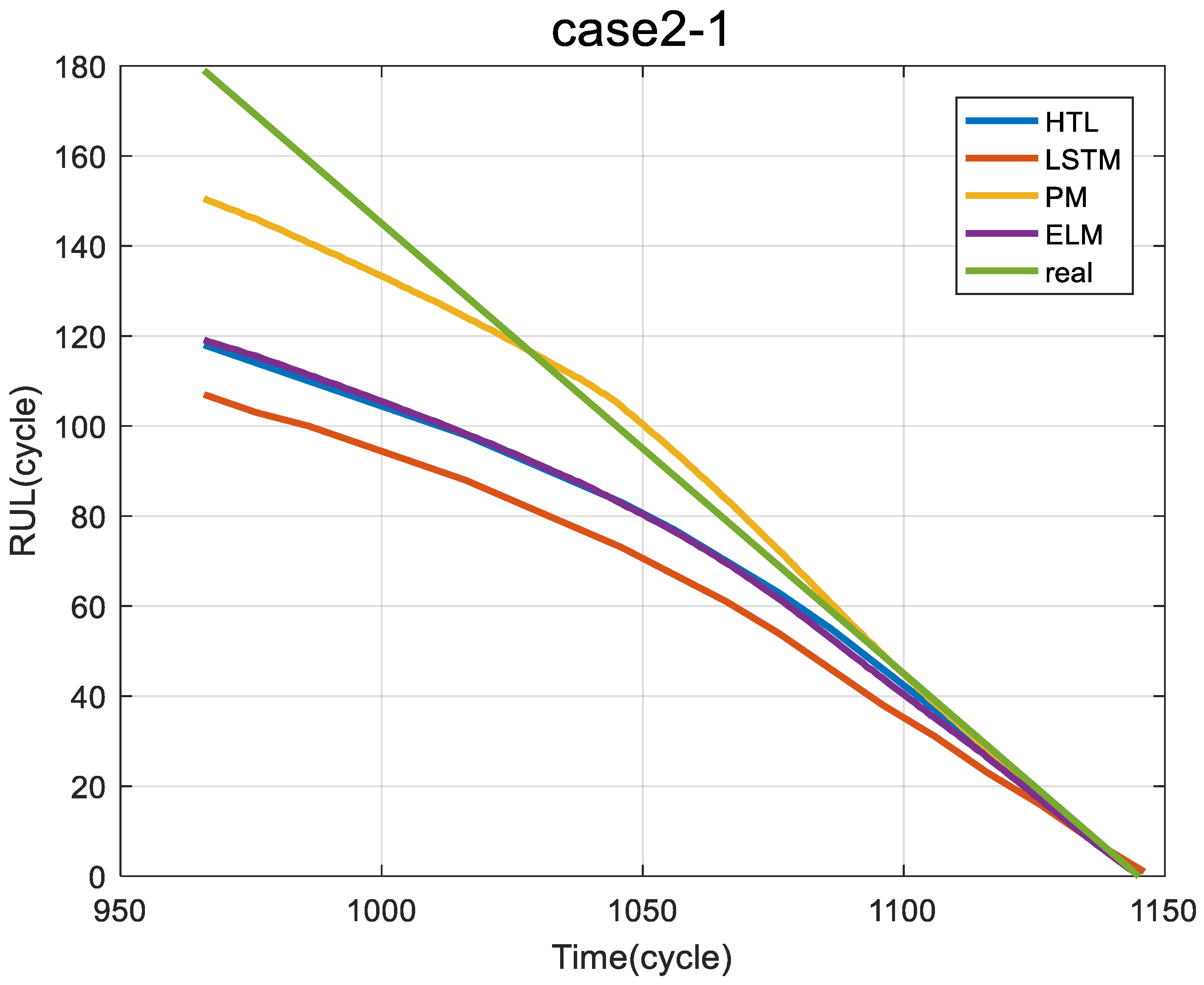
Case 2-1	6.71%	18.9%	21.5%	17.32%
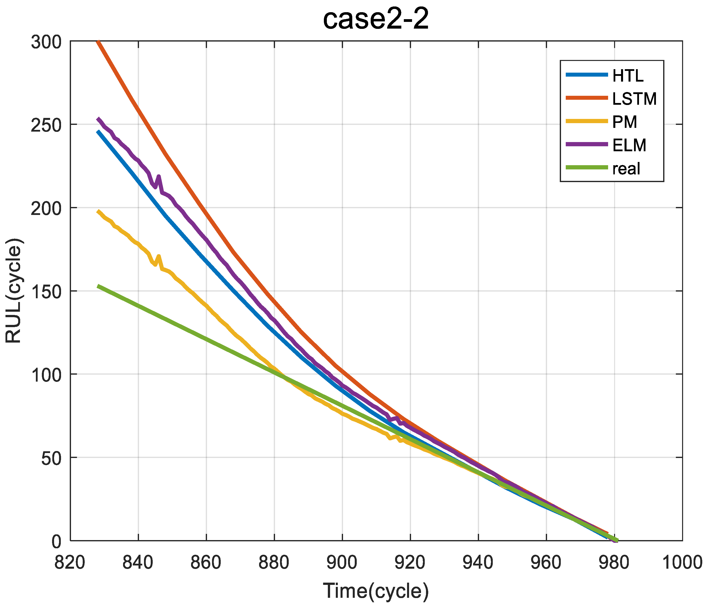
Case 2-2	8.96%	20.6%	37.6%	26.80%
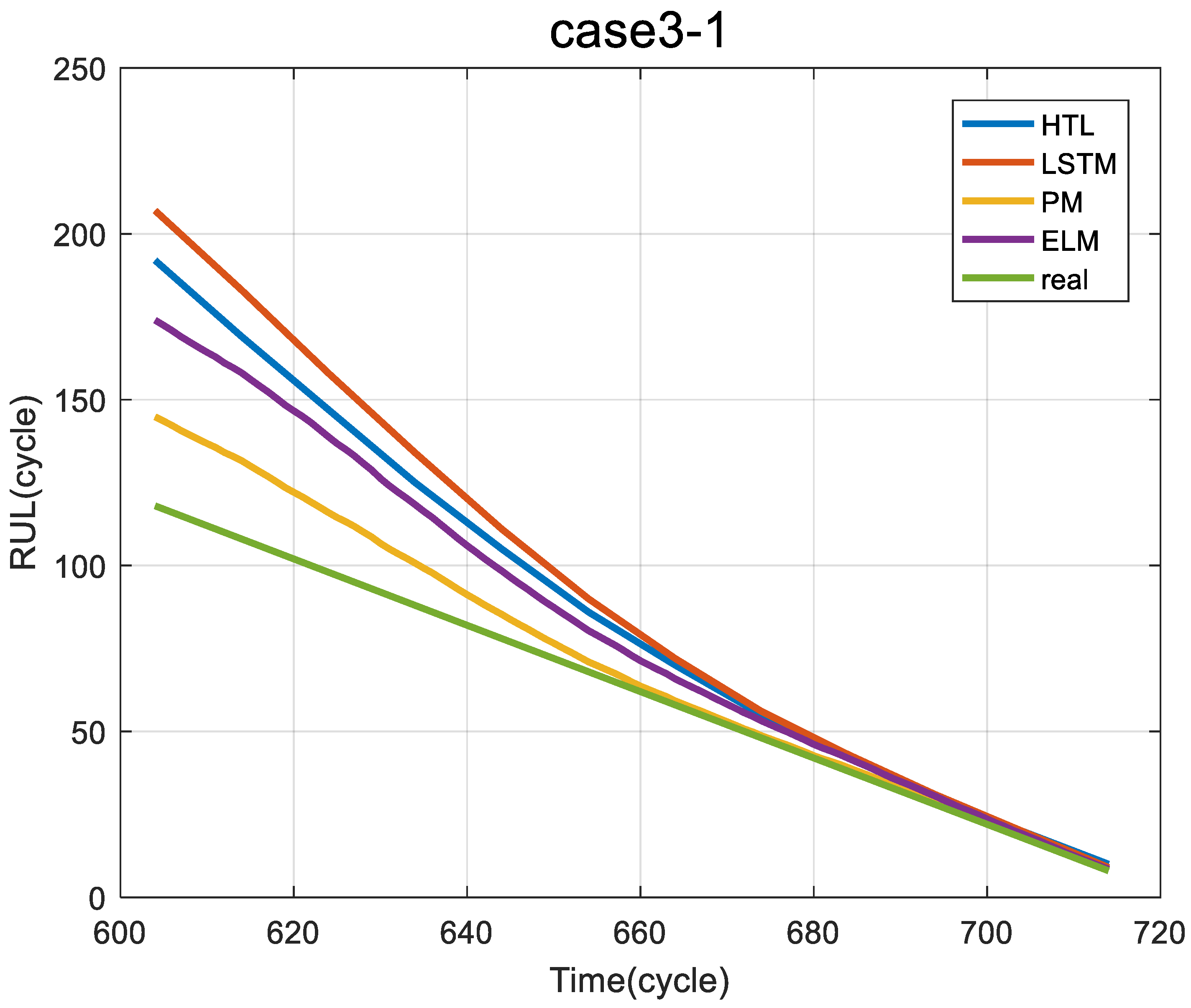
Case 3-1	8.61%	28.7%	37.2%	21.07%
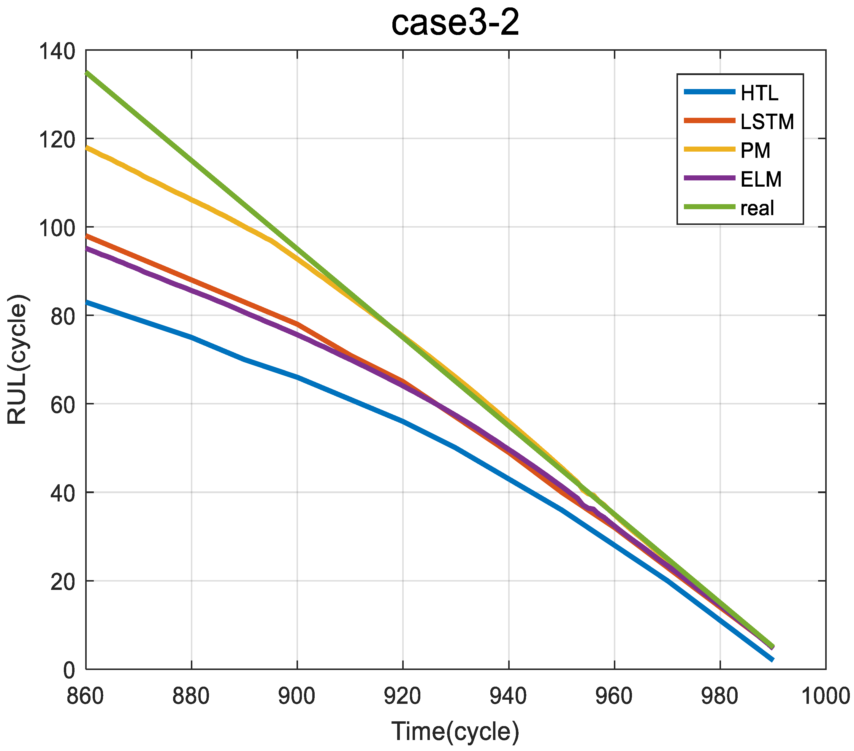
Case 3-2	6.21%	27.6%	15.6%	15.90%
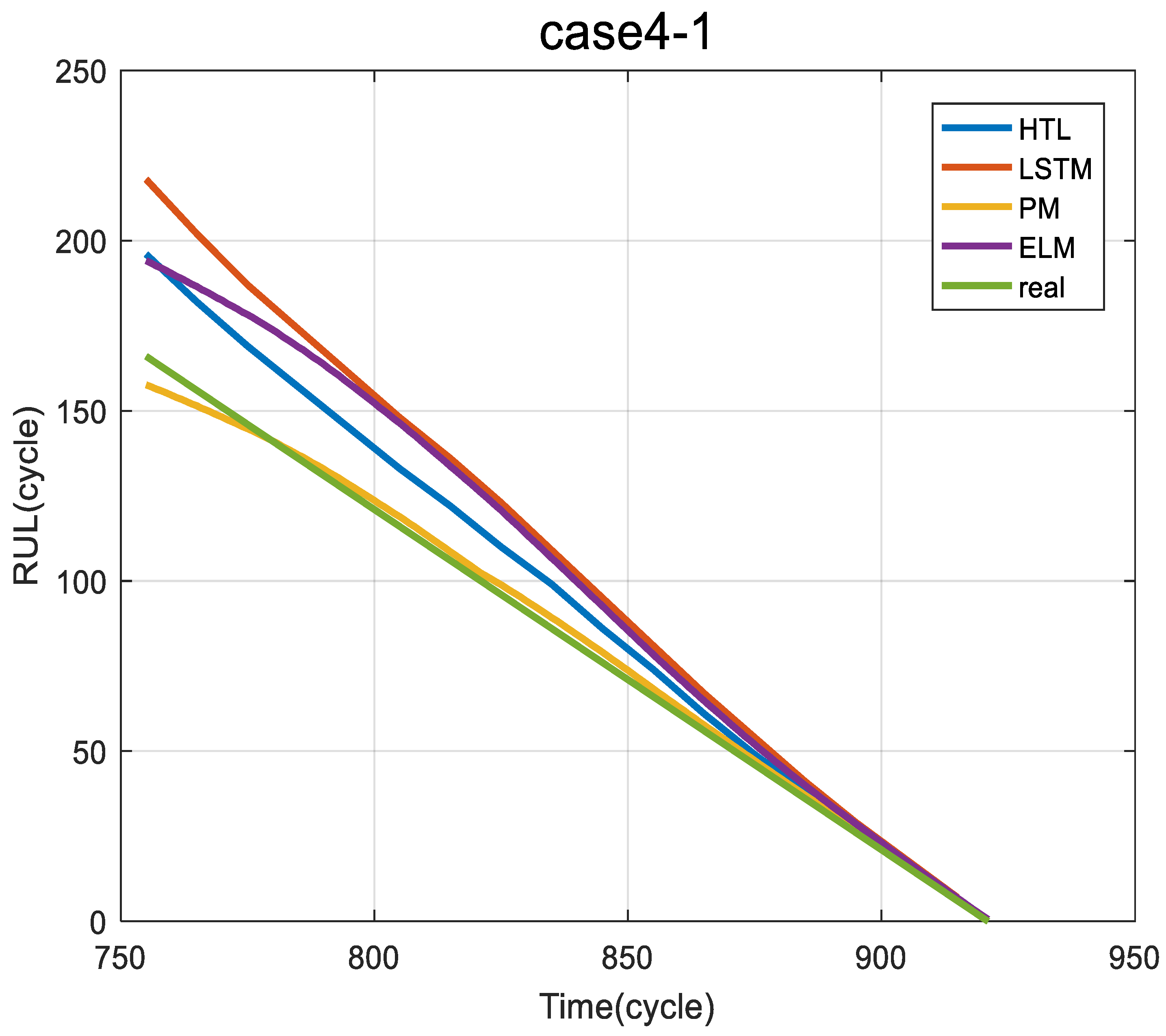
Case 4-1	3.96%	10.9%	23.6%	18.91%
Case 4-2	2.64%	20.2%	25.5%	16.05
Average	6.15%	18.96%	22.65%	17.18%

, where the MAPE is calculated by:

$$\mathrm{MAPE}=\frac{1}{n}{\sum }_{i=1}^n\frac{{|r}_{prediction,i}-r_{real,i}|}{r_{real,i}}$$

(15)

where $r_{prediction,i} \mathrm{i}\mathrm{s}$ the ith value of the RUL prediction, $r_{real,i}$ is the ith value of the real RUL, and n is the total number of predicted points.

4. Discussion

According to the samples, the degradation characteristics for the batteries in case 1 and case 4 are basically smooth and do not change dramatically with time, but the individual differences of each battery in each case are clear: one’s capacity is constantly higher than the other through the whole degradation process. Thus, such conditions are suitable for the use of the degradation rate to describe batteries’ individual differences. It is demonstrated in Table 2 that the proposed method has an obviously higher prediction accuracy in cases 1 and 4 compared with the other four methods. In case 1-2, the prediction error of the HTL method is a bit lower than the proposed method, but under overall consideration, the error of the proposed method is significantly lower than the others. When it comes to cases 2 and 3, the capacity of the two batteries in each group has a cross-point, which means the degradation rate fluctuates and has more complex individual differences. As a result, higher errors can be witnessed among all methods, but our proposed method still controls the MAPE under 10%; meanwhile, other methods have errors as high as 30%.

Overall, according to the figure and numerical analysis, the proposed method has a better prediction performance and can be applied to overcome errors caused by individual differences efficiently.

5. Conclusions

The proposed method introduced a model to identify the individual differences in lithium batteries through the capacity degradation rate. The method is based on the extreme learning machine, which is used twice: once between the capacity degradation rates and capacity to obtain adjusting factor and another time between the capacity and the RUL. The RUL is adjusted by the adjusting factor in order to reduce the error caused by individual differences.

The proposed method can clearly identify the individual differences between the historical battery and the target by making a prediction between the degradation rate and the capacity, which reduces the error caused by individual differences.

In the case study stage, three comparisons are made. Compared with the prediction with the traditional ELM model, the proposed model has a 65.66% reduction in error. Compared with some existing methods, the proposed model has 68.89% and 73.95% error reduction, respectively. In conclusion, the proposed model has a great performance in the prediction of the RUL.

References

- Chen, X.; Liu, Z. A long short-term memory neural network based Wiener process model for remaining useful life prediction. Reliab. Eng. Syst. Saf. 2022, 226, 108651. [Google Scholar] [CrossRef]
- Chen, X.; Liu, Z.; Wang, J.; Yang, C.; Long, B.; Zhou, X. An Adaptive Prediction Model for the Remaining Life of an Li-Ion Battery Based on the Fusion of the Two-Phase Wiener Process and an Extreme Learning Machine. Electronics 2021, 10, 540. [Google Scholar] [CrossRef]
- Zhang, S.J.; Kang, R.; Lin, Y.H. Remaining useful life prediction for degradation with recovery phenomenon based on uncertain process. Reliab. Eng. Syst. Saf. 2021, 208, 1. [Google Scholar] [CrossRef]
- Kauwe, S.K.; Rhone, T.D.; Sparks, T.D. Data-Driven Studies of Li-Ion-Battery Materials. Crystals 2019, 9, 54. [Google Scholar] [CrossRef]
- Liu, K.; Shang, Y.; Ouyang, Q.; Widanage, W.D. A data-driven approach with uncertainty quantification for predicting future capacities and remaining useful life of lithiumion battery. IEEE Trans. Ind. Electron. 2021, 68, 3170–3180. [Google Scholar] [CrossRef]
- Sadabadi, K.K.; Jin, X.; Rizzoni, G. Prediction of remaining useful life for a composite electrode lithium ion battery cell using an electrochemical model to estimate the state of health. J. Power Sources 2021, 481, 228861. [Google Scholar] [CrossRef]
- Zhang, Y.; Chen, L.; Li, Y.; Zheng, X.; Chen, J.; Jin, J. A hybrid approach for remaining useful life prediction of lithium-ion battery with adaptive levy flight optimized particle filter and long short-term memory network. J. Energy Storage 2021, 44, 103245. [Google Scholar] [CrossRef]
- Zhou, Y.; Gu, H.; Su, T.; Han, X.; Lu, L.; Zheng, Y. Remaining useful life prediction with probability distribution for lithium-ion batteries based on edge and cloud collaborative computation. J. Energy Storage 2021, 44, 103342. [Google Scholar] [CrossRef]
- Aivaliotis, P.; Georgoulias, K.; Chryssolouris, G. A RUL calculation approach based on physical-based simulation models for predictive maintenance. In Proceedings of the 2017 International Conference on Engineering, Technology and Innovation (ICE/ITMC), Madeira, Portugal, 27–29 June 2017; pp. 1243–1246. [Google Scholar] [CrossRef]
- Yang, S.; Tang, B.; Wang, W.; Yang, Q.; Hu, C. Physics-informed multi-state temporal frequency network for RUL prediction of rolling bearings. Reliab. Eng. Syst. Saf. 2024, 242, 109716, ISSN 0951-8320. [Google Scholar] [CrossRef]
- Gao, D.; Zhou, Y.; Wang, T.; Wang, Y. A Method for Predicting the Remaining Useful Life of Lithium-Ion Batteries Based on Particle Filter Using Kendall Rank Correlation Coefficient. Energies 2020, 13, 4183. [Google Scholar] [CrossRef]
- Osama, T.M.; Haider, N.I.; Zubair, K.; Michal, P. Accurate prediction of remaining useful life for lithium-ion battery using deep neural networks with memory features. Front. Energy Res. 2023, 11, 1059701. [Google Scholar]
- Gao, D.; Huang, M. Prediction of Remaining Useful Life of Lithium-ion Battery based on Multi-kernel Support Vector Machine with Particle Swarm Optimization. Korea Sci. 2017, 17, 1288–1297. [Google Scholar]
- Zhang, H.; Hu, C.-H.; Du, D.-B.; Pei, H.; Zhang, J.-X. Remaining Useful Life Prediction Method of Lithium-Ion Battery Based on Bi-LSTM Network Under Multi-State Influence. Acta Electron. Sin. 2022, 50, 619–624. [Google Scholar]
- Ren, L.; Zhao, L.; Hong, S.; Zhao, S.; Wang, H.; Zhang, L. Remaining Useful Life Prediction for Lithium-Ion Battery: A Deep Learning Approach. IEEE Access 2018, 6, 50587–50598. [Google Scholar] [CrossRef]
- Ansari, S.; Ayob, A.; Hossain Lipu, M.S.; Hussain, A.; Saad, M.H.M. Data-Driven Remaining Useful Life Prediction for Lithium-Ion Batteries Using Multi-Charging Profile Framework: A Recurrent Neural Network Approach. Sustainability 2021, 13, 13333. [Google Scholar] [CrossRef]
- Tang, X.; Wan, H.; Wang, W.; Gu, M.; Wang, L.; Gan, L. Lithium-Ion Battery Remaining Useful Life Prediction Based on Hybrid Model. Sustainability 2023, 15, 6261. [Google Scholar] [CrossRef]
- Daniel, P.; Jon, A.; Iker, C.; Aitor, H.; Iñigo, U.; Aitor, D.Z. Data-driven methodology for optimal Lithium-ion battery RUL prediction. Energy 2023, 2. [Google Scholar] [CrossRef]
- Pan, C.; Chen, Y.; Wang, L.; He, Z. Lithium-ion Battery Remaining Useful Life Prediction Based on Exponential Smoothing and Particle Filter. Int. J. Electrochem. 2019, 14, 9537–9551. [Google Scholar] [CrossRef]
- Hou, E.; Wang, Z.; Qiao, X.; Liu, G. Remaining useful cycle life prediction of lithium-ion battery based on TS fuzzy model. Front. Energy Res. 2022, 10, 973487. [Google Scholar] [CrossRef]
- Severson, K.A.; Attia, P.M.; Jin, N.; Perkins, N.; Jiang, B.; Yang, Z.; Chen, M.H.; Aykol, M.; Herring, P.K.; Fraggedakis, D.; et al. Data-driven prediction of battery cycle life before capacity degradation. Nat. Energy 2019, 4, 383–391. [Google Scholar] [CrossRef]
- Chen, G.-J.; Chung, W.-H. Evaluation of Charging Methods for Lithium-Ion Batteries. Electronics 2023, 12, 4095. [Google Scholar] [CrossRef]
- Wang, L.; Wang, C.; Lu, X.; Ping, D.; Jiang, S.; Wang, X.; Zhang, J. A Design for a Lithium-Ion Battery Pack Monitoring System Based on NB-IoT-ZigBee. Electronics 2023, 12, 3561. [Google Scholar] [CrossRef]
- Wang, Q.-Y.; Wang, S.; Zhou, G.; Zhang, J.-N.; Zheng, J.-Y.; Yu, X.-Q.; Li, H. Progress on the failure analysis of lithium battery. Acta Phys. Sin. 2018, 67, 128501. [Google Scholar] [CrossRef]
- Zhai, Q.; Ye, Z.S. RUL prediction of deteriorating products using an adaptive Wiener process model. IEEE Trans. Ind. Inf. 2017, 13, 2911–2921. [Google Scholar] [CrossRef]
- Cao, X.; Li, P.; Ming, S. Remaining useful life prediction-based maintenance decision model for stochastic deterioration equipment under data-driven. Sustainability 2021, 13, 8548. [Google Scholar] [CrossRef]
- Xing, Y.; Ma, E.W.M.; Tsui, K.L.; Pecht, M. An ensemble model for predicting the remaining useful performance of lithium-ion batteries. Microelectron. Reliab. 2013, 53, 811–820. [Google Scholar] [CrossRef]
- Ma, J.; Shang, P.; Zou, X.; Ma, N.; Ding, Y.; Sun, J.; Cheng, Y.; Tao, L.; Lu, C.; Su, Y.; et al. A hybrid transfer learning scheme for remaining useful life prediction and cycle life test optimization of different formulation Li-ion power batteries. Appl. Energy 2021, 282. [Google Scholar] [CrossRef]
- Zhou, Y.; Huang, Y.; Pang, J.; Wang, K. Remaining useful life prediction for supercapacitor based on long short-term memory neural network. J. Power Sources 2019, 440, 227149. [Google Scholar] [CrossRef]