Abstract
Roadbed construction typically employs layered and staged filling, characterized by a periodic feature of ‘layered filling—filling interval’. The load and settlement histories established during staged construction offer crucial insights into long-term deformation under filling loads. However, models often rely solely on post-construction settlement data, neglecting the rich filling data. To accurately predict composite foundation ground (CFG) settlement, an LSTM–Transformer deep learning model is used. Five factors from the ‘fill height–time–foundation settlement’ curve are extracted as input variables. The first-layer LSTM model’s gate units capture long-term dependencies, while the second-layer Transformer model’s self-attention mechanism focuses on key features, efficiently and accurately predicting ground settlement. The model is trained and analyzed based on the newly constructed Changsha–Zhuzhou–Xiangtan intercity railway section CSLLXZQ-1, which has a CFG pile composite foundation. The research shows that the proposed LSTM–Transformer model for the settlement prediction of composite foundations has an average absolute error, mean absolute percentage error, and root mean square error of 0.224, 0.563%, and 0.274, respectively. Compared to SVM, LSTM, and Transformer neural network models, it demonstrates higher prediction accuracy, indicating better reliability and practicality. This can provide a new approach and method for the settlement prediction of newly constructed CFG composite foundations.
1. Introduction
High-speed railway trains are particularly sensitive to the settlement and deformation of the underlying track structure, especially when traveling at high speeds [1,2]. Therefore, controlling the post-construction settlement of high-speed railway embankments has become a crucial aspect of high-speed railway embankment design. The use of cement fly ash gravel (CFG) piles to treat soft soil foundations at the location has advantages such as minimal settlement, high strength, and short construction period. It has become a frequently employed method in the construction of high-speed railways [3,4,5]. For composite foundations commonly encountered in high-speed railway construction, such as CFG pile composite foundations, accurately predicting their post-construction settlement is a key aspect of high-speed railway construction and settlement assessment work [6,7].
Currently, there are mainly three categories of traditional foundation settlement prediction methods: The first category involves using theoretical methods, such as the layer sum method, to calculate the final settlement, then simplifying the consolidation formula to estimate the degree of consolidation, thereby predicting the development pattern of settlement; the second category is the numerical calculation method, which is based on consolidation theory and combined with various soil constitutive models to calculate the final amount of settlement and its development pattern. Both of these methods are theoretically reasonable and feasible, but the calculation parameters involved must be obtained through experiments. During the sampling process, the soil samples are inevitably disturbed, leading to discrepancies between experimental and actual parameters. Therefore, the prediction results of these two methods usually have large errors. The third category includes methods such as the hyperbolic method [8], Asaoka’s method [9], Poisson’s method [10], and the grey model method [11]. Since most of these prediction methods and models are singular and each has its characteristics and applicable scenarios, they cannot fully exploit the information of actual measurement data, and the accuracy of their predictions still needs to be improved.
With the development of computer science technology, more scholars are utilizing the powerful nonlinear fitting capabilities of algorithms such as artificial neural networks and support vector machines [12,13,14] for the deformation prediction of foundations. Liu Yulin [15] established a sparrow search algorithm optimized support vector machine regression (SSA-SVR) prediction model to forecast the settlement of coal gangue subgrade. Chen Weihang et al. [16], based on the bidirectional long short-term memory network (Bi-LSTM), combined a rolling iteration method to update settlement predictions, which can effectively enhance the reliability of subgrade settlement forecasting. Zhu Jianmin et al. [17], based on the GA-BP neural network model, predicted the post-construction settlement of loess high-fill sites. Li Tao et al. [18] proposed a subway tunnel surface settlement prediction method using VMD-GRU for step-method construction, which can effectively predict short-term abrupt data changes.
The aforementioned combined neural network models have achieved certain results in learning and predicting surface settlement data. However, these intelligent algorithms also have some shortcomings. For instance, support vector machines struggle with large sample data, and although neural networks have strong fitting capabilities, they face issues such as overfitting, local minima, or slow convergence during the training process. Therefore, there is a need to improve existing methods. Furthermore, they usually only use post-construction subgrade settlement data as sample information, ignoring the rich construction knowledge during the filling period. Subgrades often adopt the periodic characteristics of ‘layered filling—filling intervals’, and the post-construction settlement can be considered as a long filling interval. By incorporating construction period filling information into the training set, it is possible to better extract data features and improve the prediction of the foundation, thereby effectively guiding construction. More classic cases should be added.
By comparing and analyzing various neural network models used in existing settlement prediction studies, it was found that the long short-term memory (LSTM) networks [19,20], due to their superior memory retention and selection capabilities, effectively handle nonlinear relationships within data and capture long-term dependencies among data points. They have been extensively applied in predicting landslide displacement [21], dam deformation [22], and stable parameters for tunnel boring machines [23], and modeling the evolution of shear behavior between soil and structural surfaces [24], among other applications. Based on these studies, this paper proposes a new LSTM–Transformer-based CFG composite foundation settlement prediction model. In this model, the first layer uses the gating mechanism of the LSTM to perceive coupling features related to the settlement rate in the sequence. After obtaining a comprehensive dependency relationship, it is transmitted to the Transformer layer. The Transformer, through self-attention, focuses on more crucial task information. With supervised training on extensive data, it resists the impact of noise and outliers, emphasizing important factors in long-term multivariate sequences, thereby improving prediction accuracy and the model’s generalizability. Currently, the LSTM–Transformer model has been applied in fields like solar power generation forecasting [25], prediction of the remaining life of rolling bearings [26], and short-term electric load forecasting for industrial users [27], but it has not yet been applied in the field of foundation settlement.
This paper, based on the LSTM–Transformer model, takes the newly constructed Chang–Zhu–Tan Intercity Railway and the Chang–Shi Railway connecting line’s high fill CFG pile composite foundation engineering as the background. It integrates information observed during the construction period to perform foundational settlement modeling and predictive analysis. Additionally, traditional machine learning models—SVM, LSTM, and Transformer—are used for comparative analysis of settlement predictions.
2. Monolithic Framework
Based on foundation settlement monitoring data, an LSTM–Transformer model for settlement prediction was constructed, as shown in Figure 1. The advantage of this model lies in its ability to deeply mine the sequence-related features hidden in foundation deformation monitoring data. It achieves the integration of temporal features and influencing factors, dynamically measures the contribution of each factor to the deformation, and explores the reasons behind changes in the deformation effects. By fully utilizing the rich dataset of subgrade settlement measurements for post-construction foundation settlement prediction, this model can provide references for subgrade engineering scheme design, saving the time and financial resources required for construction.
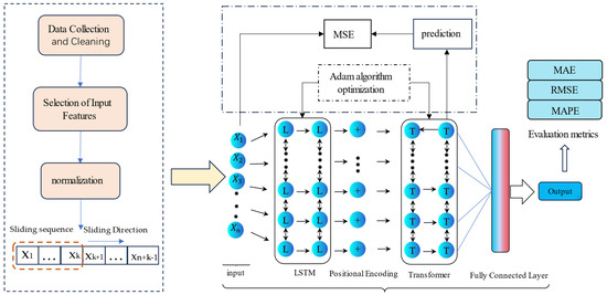
Figure 1.
The overall framework of the LSTM–Transformer-based foundation prediction model.
3. The Establishment of a CFG Compound Foundation Settlement Model Based on LSTM–Transformer
3.1. The Transformer Model
The Transformer is a network that leverages attention mechanisms to enhance the speed of model training. Its encoder component resembles a large multilayer perceptron (MLP) [28], where data can be input simultaneously and processed in parallel. Its remarkable capability in handling long sequential data makes it effective for predicting settlement. Moreover, it addresses the issue of gradient explosion efficiently, rendering it suitable for settlement prediction tasks.
The Transformer relies entirely on self-attention mechanisms to extract inherent features. It can learn long-term dependencies and is more easily parallelizable compared to RNN-type models. The original Transformer was used in classification tasks, obtaining high-dimensional features for individual time steps through an embedding layer. It uses positional encoding to retain the positional information from the original sequence [27,29]. Subsequently, based on the query–key–value concept, the self-attention layer maps the original features into three components: Q, K, and V. It computes the correlation between features at different time steps and the current moment using Q and , then derives the features for the next time step through a weighted sum of . The self-attention mechanism’s computational formula [30] in the Transformer is shown as follows:
In the equations, represents the output sequence of multi-head attention; denotes the dimension of (), (), and (); is the scaling factor; , , , and are matrices for linear transformations; represents the query calculation vector; represents the vector for which the query is computed; denotes the current actual features; represents the attention weights, obtained through scaled dot-product output vector sequences.
The multi-head self-attention mechanism is an improvement of the self-attention mechanism. It divides the self-attention into multiple parallel heads that perform linear mappings multiple times. It calculates attention for different mapping results, processing different levels of information in the input sequence and computing global attention. Essentially, it is an integration of multiple independent self-attentions. The Transformer not only provides one of the predictions for foundation settlement through the self-attention mechanism algorithm, but its multi-head attention mechanism can also repeat the algorithm multiple times to obtain more balanced and goal-aligned results. During the training and prediction process, the Transformer internally learns and trains with the provided data, effectively extracting intrinsic information from the data. In predictive training, it can mask the original data to enhance the persuasiveness of the algorithm’s predictions. Figure 2 shows the structural diagram of the multi-head attention mechanism.
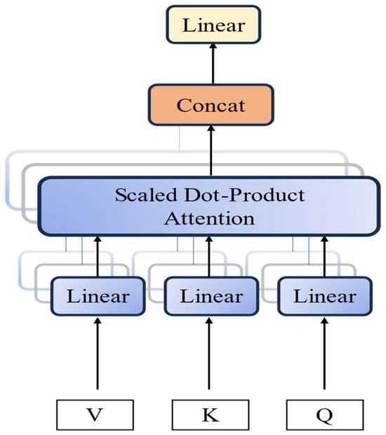
Figure 2.
Multi-head mechanism.
3.2. The LSTM Model
LSTM (long short-term memory) is a type of sequence data processing model that addresses the issues of vanishing and exploding gradients encountered in training long sequences within RNNs (recurrent neural networks) by introducing ‘gates’ mechanisms [31]. The LSTM model implements selective information flow through these gates—the forget gate, input gate, and output gate—which control the retention, input, and output of information, respectively. This architecture allows the LSTM to maintain long-term dependencies and handle information flow more effectively compared to traditional RNNs. The basic structure of an LSTM network, as depicted in Figure 3, showcases its recurrent nature. Through its distinctive ‘gates’, the LSTM can manage and control the cell state [32,33]:
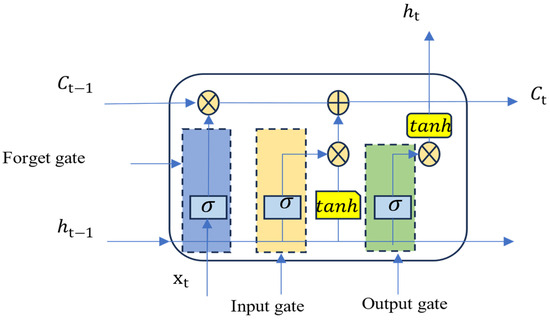
Figure 3.
LSTM recurrent neural network diagram.
In the equations, represents the LSTM update value (input gate); is the new candidate value vector (candidate value); and represent the cell states of the previous and current rounds, respectively; and represent the hidden states of the previous and current rounds, respectively; w and b represent the weight matrices and bias terms of the output gate, input gate, and forget gate, respectively.
In summary, the current time step’s hidden layer output () and cell state () in the LSTM are jointly determined by the previous time step’s hidden layer output (), cell state (), and the current time step’s input (). Additionally, according to relevant research, when exploring the complex nonlinear relationship between foundation settlement and influencing factors, it is possible to construct LSTM models with two or more stacked hidden layers for training.
3.3. The LSTM–Transformer Model Structure
In time series tasks, there are typically two challenges: short-term dependencies and long-term dependencies. When future data is primarily influenced by historical data over a longer time span, this situation is referred to as long-term dependency. Conversely, when future data is mainly influenced by historical data over a shorter time span, this is referred to as short-term dependency.
The LSTM processes data sequentially over time, relying on the memory of its cell state to propagate dependencies between time steps. Due to the potential loss of information within this process, LSTMs are adept at capturing short-term dependencies within sequences. However, their effectiveness in capturing long-term dependencies within sequences is relatively limited, leading to challenges in addressing long-term dependency issues [34].
The Transformer model utilizes self-attention mechanisms to model relationships between different time steps. Due to its parallelized mechanism for extracting both short-term and long-term information, the Transformer does not exhibit bias towards recent time points, meaning it does not assign higher weights to the most recent data [35]. The parallel attention mechanism allows for the extraction of features from distant time steps. However, the parallel nature of the Transformer also introduces a challenge—it does not inherently capture sequential information in its input due to the lack of an explicit temporal order.
Considering the two points mentioned above, a hybrid LSTM–Transformer model is proposed to effectively combine the ability of the LSTM to capture short-term sequential dependencies and the modeling capability of the Transformer for relationships between time steps, especially long-term dependencies. In this architecture, an LSTM encoder is used to encode the input sequence, while a Transformer decoder is employed to generate the output sequence. With this structure, the LSTM decoder can gradually produce the output sequence to retain temporal features, while the Transformer encoder can effectively capture relationships between different positions in the multivariate time series, thereby enhancing the overall model performance.
The LSTM–Transformer architecture diagram is shown in Figure 4, and the specific process is as follows:
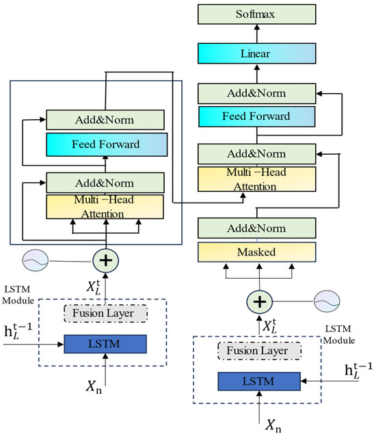
Figure 4.
The LSTM−Transformer architecture diagram.
- (1)
- Data processing
The frequency of foundation monitoring changes over the operation time, with a higher frequency in the initial stages of construction and a lower frequency later on. The settlement observation data is a set of non-equidistant data, which does not allow for equidistant analysis. The use of cubic spline interpolation with segmented interpolation significantly reduces the number of interpolations, facilitating the solution of the undetermined coefficients and resulting in a smoother curve. During the settlement monitoring process, accidental factors such as bad weather or instrument failure may cause some settlement observation data to deviate from normal. These anomalies can be determined based on the overall trend of the settlement curve. It is advisable to first clean and eliminate these data before proceeding with interpolation.
- (2)
- Selection and Standardization of Input Features
To predict settlement at time t, it is necessary to use settlement data before time t as inputs. The model’s training effectiveness depends on these input variables. More input data extracted from the settlement–time curve helps the model’s hidden layers learn complex, nonlinear relationships, improving predictions. The next moment’s subgrade settlement trend is often closely related to the immediate past settlement. Considering this, the past 3, 6, 9 days’ settlements amount to , , and ; the settlement rate and fill height are selected as key factors.
Considering that foundation settlement data is multivariate, with differences in dimensions and numerical values, directly applying it can affect model training and testing. Therefore, based on the formula, the original model is normalized to ensure that the numerical ranges of different variables are the same. This reduces biases and unequal weight distribution towards the data, thereby improving model accuracy and training speed.
- (3)
- A sliding time window is used to segment normalized time series, with the calculation formula as follows:
In the equations, represents the normalized cumulative settlement; represents the segmented sliding sequence.
- (4)
- The segmented time series is input into the LSTM–Transformer model.
The LSTM neural network layer is used to capture non-linear information hidden in cumulative settlement values at different times. This process yields new cell memory state information for each time step. At this point, the output hidden state vector is combined with the original input through a fusion layer, integrating different features learned from multiple layers and directions of the LSTM. This results in a more comprehensive and accurate representation, which is then used as input to the multi-head attention layer. During the calculation of the multi-head attention (MHA), the input from the previous module and the current input are jointly considered.
The structure of the Transformer network layer is constructed, utilizing the self-attention mechanism of the Transformer to allocate weights for information exploration by the LSTM. Subsequently, in the feature layer, the input is reconstructed, learning the previous time step states and incorporating factors such as the current observed fill height to predict future foundation settlement. The calculation process is shown in Equations (11)–(13):
In the equations, represents the time series group processed by the LSTM module; is the memory output module representing each output from the LSTM module without gradient updates; represents the output, denoted as and , from the LSTM module without gradient updates, continuously fed into the multi-head attention (MHA) layer, constantly introducing the hidden states from the previous LSTM module into the current input. In Equation (12), represents the output of the fusion layer; F denotes the combination of optional values and in the fusion layer; signifies that the vector added in the multi-head attention (MHA) undergoes the same computational process [36].
In Equation (13), represents the settlement prediction values output by the LSTM–Transformer model. The fusion layer combines the output vector with the corresponding input vector. The fused vector is then passed through an activation function, aiding the model in allocating attention weights based on various input features.
3.4. Accuracy Evaluation Method
The model prediction first involves fitting the data to establish the model and then making subsequent data predictions based on the established model. Fitting is the key, and prediction is the result. This article mainly evaluates the quality of the prediction results using three indicators: mean absolute error (MAE), mean absolute percentage error (MAPE), and root mean square error (RMSE). The calculation formulas are as follows:
In the formula, represents the actual measured settlement at time (t); is the predicted settlement at time (t); is the average of () measured settlement values; and n is the number of samples. Among them, the smaller and closer to 0 the values of MAE, MAPE, and RMSE, the higher the accuracy of the model training section
4. Engineering Example
4.1. Engineering Overview
This text describes a composite foundation engineering project using CFG piles for the CSLLXZQ-1 section of the newly constructed Changsha–Zhuzhou–Xiangtan intercity railway and the Chang–Shi railway connection line. The project spans from DK23 + 200 to DK23 + 350 in a test area with an average embankment height of 16 m, surrounded by complex features such as farmlands and ponds. The soil layers in the test area, from top to bottom, include subgrade soil, cushion soil, miscellaneous fill surface soil, silty clay, powdery clay, coarse sand, gravelly sand, and gravelly silty clay. CFG piles, with a diameter of 0.5 m, spaced 0.8 m apart, and an effective length of 15 m, are employed for foundation reinforcement in a square arrangement, as shown in Figure 5. The subgrade soil settlement is monitored using observation piles, while the settlement of the CFG pile composite foundation is observed through settlement plates. Four sections were chosen for the subgrade settlement observation piles, labeled as DK23 + 200, DK23 + 250, DK23 + 300, and DK23 + 350. Each section has three settlement observation piles, named according to the section mileage + G1 (G2, G3). Additionally, settlement plates are positioned at four locations along the observation sections, named according to the section mileage + L1. As illustrated in Figure 6 below, one most representative observation points is selected for predictive analysis in each section. As shown in Figure 7, Figure 7a is an onsite installation diagram of the settlement observation pile, and Figure 7b shows the onsite observation of foundation settlement using a level instrument. The geometric dimensions of the typical section are shown in Figure 8. The physical and mechanical parameters of each soil layer are shown in Table 1.
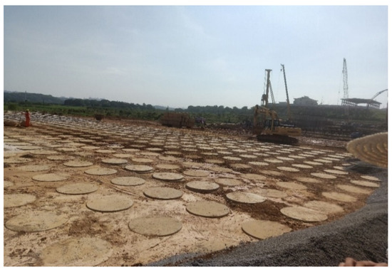
Figure 5.
Site map of CFG pile composite foundation.
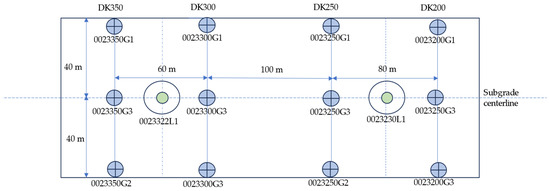
Figure 6.
Layout diagram of monitoring points.
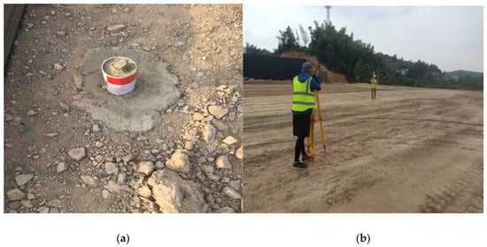
Figure 7.
CFG pile composite foundation observation device—settlement plate on-site photo.
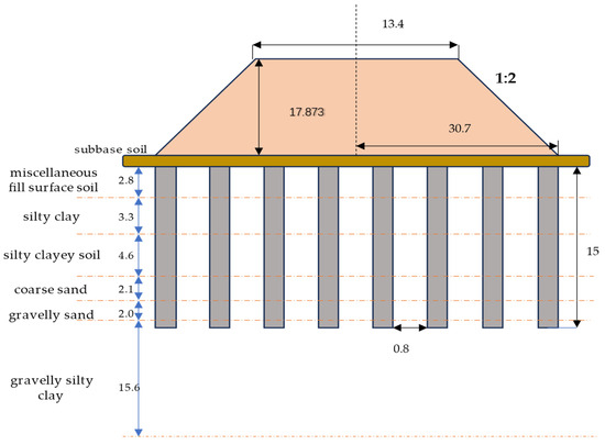
Figure 8.
Schematic diagram of typical section geometry.

Table 1.
Soil parameters table.
The significant variation in the ground settlement rate during both the construction and post-construction periods of this high-fill CFG pile composite foundation made it challenging to maintain a consistent monitoring frequency. Consequently, the data obtained from on-site monitoring was non-uniform in timing, rendering it unsuitable for temporal analysis. To meet the requirements for temporal analysis, the original monitoring data underwent equidistant processing using a cubic spline interpolation method. Considering the precision and efficiency of neural network training, the data was processed into equidistant settlement records at intervals of 24 h, comprising a total of 160 observation points. The resulting interpolated ground settlement data is illustrated in the following Figure 9.
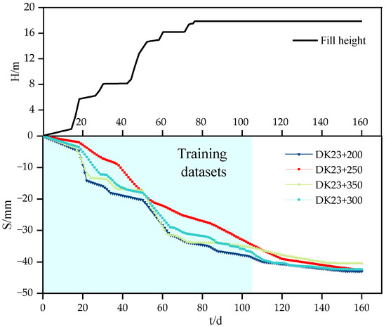
Figure 9.
Relationship between fill height, time, and ground settlement.
From Figure 9, it can be observed that the settlement curves of the four typical monitoring sections exhibit a distinctive ‘step’ shape over time. Specifically, as the embankment height increases, the settlement of the composite foundation also increases. As the current stage of embankment construction is completed, the rate of increase in settlement of the composite foundation slows down. Additionally, it can be noted that the settlement rates of the four typical monitoring sections show a similar pattern. In the early stages of embankment construction, the consolidation rate of the composite foundation soil is relatively fast. As the upper load increases, the composite foundation soil gradually densifies, resulting in a gradual slowing of the settlement rate, ultimately reaching a stable state.
The magnitude range of input and output values significantly influences the predictive performance of the model mentioned above. Therefore, the original model is normalized based on the formula, and after normalization, a sliding window approach with a window size of k = 15 is applied to generate the model’s input sequence.
Grey relational analysis [37] is a method that involves normalizing the original data and measuring the correlation and similarity between factors by calculating the correlation coefficient and determining the degree of association. The grey relational grade (GRG) is employed to assess the degree of correlation between each input value and the settlement amount of the CFG pile composite foundation. A GRG value closer to 1 signifies a higher degree of correlation between the two; when the GRG value exceeds 0.6, the correlation between them is considered extremely high. If the GRG value falls within the range of 0.5 to 0.6, it indicates a correlation between the two factors. When the GRG value is less than 0.5, it suggests a lack of correlation between them [16].
Using , , , , and as the model’s input, Table 2 illustrates the grey relational grades between each influencing factor and the settlement of the CFC piles. From Table 2, it is evident that factor , , exhibits notably high grey relational grades concerning the settlement at all four monitoring points, with GRGs exceeding 0.96. Similarly, factor b demonstrates a close correlation with the settlement of the CFG pile composite foundation, showing GRGs above 0.90 across all four monitoring points. The above indicates that the selection of the five variable factors is reasonable.
Table 2.
Analysis of grey relational coefficient for each section.
The learning capability and prediction performance of the model sequence are influenced by the length of the input sequence. If the sequence is too short, the neural network model may struggle to effectively extract the intrinsic features of the data. On the other hand, if the sequence is too long, it increases the complexity of information and makes feature extraction more challenging. Therefore, selecting an appropriate length for the model sequence is crucial [16]. In this study, the first 150 data points were chosen, following the principle of using 70% of the data as the training set and 30% as the validation set. Consequently, the training set consists of the initial 105 data points, which are used for training, and the subsequent data points (106th to 150th) are used for prediction.
4.2. Analysis of Prediction Results
The results obtained in this experiment were achieved using the PyTorch deep learning framework, implementing a LSTM-Transformer encoder–decoder model. The implementation was carried out in the Python programming language, on a Windows 10 operating system, using the PyCharm development environment. The experimental setup included an NVIDIA GeForce RTX 3090Ti graphics card, an Intel(R) i7-13700k CPU, and 64 GB of memory. The LSTM–Transformer model was applied to predict and analyze four cross-sections: DK23 + 200, DK23 + 250, DK23 + 300, and DK23 + 350. The network training utilized the Adam optimization algorithm, with mean squared error loss (MSELoss) as the loss function. The learning rate was set to 0.001, and parameter tuning was performed using grid search. Specific parameter settings are detailed in the Table 3. The prediction results obtained after 200 iterations are illustrated in Figure 10 and Figure 11.
Table 3.
Model hyperparameter settings.
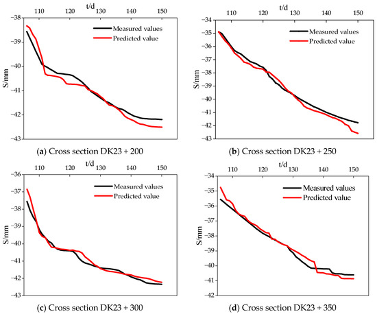
Figure 10.
LSTM–Transformer model settlement prediction results.
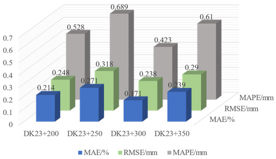
Figure 11.
The predictive performance indicator results at each point.
During the filling phase, the foundation settlement curve shows a stair-step characteristic as filling progresses. Traditional machine learning and Transformer models capture this feature poorly, whereas the LSTM and LSTM–Transformer models can effectively recognize it. As shown in Figure 12, the SVM model is not sensitive enough to capture local steps or convergence features. Meanwhile, the self-attention mechanism of the Transformer model can effectively utilize the internal correlations of the sequence for better modeling. Additionally, as seen in Figure 13, the predictive indices RMSE, MAPE, and MAE of the SVM model are 1.395 mm, 2.807%, and 1.15, respectively, indicating the worst predictive performance. Compared to SVM, its predictions are more accurate. Due to its parallel attention mechanism, it can extract more distant temporal features, resulting in better convergence in final settlement predictions. However, it lacks a certain bias ability and does not assign higher weights to the most recent data points. As known from Figure 12, after 120 days, its predicted settlement changes less compared to other models, with the final prediction being lower than the actual value.
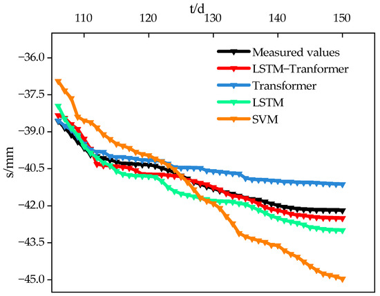
Figure 12.
The settlement prediction results of different models.
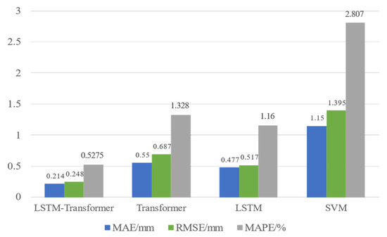
Figure 13.
The prediction metrics of different models.
The LSTM model, with its unique gating mechanisms like forget gate, input gate, and output gate, has strong memory capability and can adaptively mine historical information about foundation settlement and various influencing factors. Its prediction results in terms of MAE, RMSE, and MAPE are improved by 13.3%, 24.7%, and 12.6%, respectively, compared to the Transformer model, thus better predicting foundation settlement. In the LSTM−Transformer model, the LSTM layer extracts historical state features for global learning and weight distribution, while the Transformer layer’s multi-head self-attention mechanism performs feature extraction and fusion at multiple levels. The diverse features extracted pay special attention to and learn from key factors like filling height, enhancing the capture of the early-stage filling height’s effect on the physical and mechanical structure changes of the geotechnical body. As seen from the predictive effects of the four sections in Figure 10, the predictions closely fit the actual values, with each point’s prediction being consistent with the actual deformation trend. As known from Figure 11, the LSTM–Transformer model has the lowest average absolute error (MAE), average absolute percentage error (MAPE), and root mean square error (RMSE) of 0.224, 0.563%, and 0.274, respectively, among the four models, making it the most accurate in prediction and the best in feature matching.
5. Conclusions
This paper proposes a CFG composite foundation settlement prediction model based on the LSTM–Transformer model. The model is validated using the foundation settlement data monitored from the CFG pile composite foundation engineering of the CSLLXZQ-1 section of the newly constructed Chang−Zhu−Tan Intercity Railway, leading to the following conclusions:
- (1)
- During the construction period of high fill embankments, there is a periodic characteristic of layered filling and intervals between fillings. Compared to the other three models, the LSTM–Transformer model is better at capturing this cyclical feature, with its prediction curve displaying a pronounced step-like characteristic. In contrast, the other three models, influenced by prior information, cannot quickly adapt, and their predictions gradually converge to the observed values over time.
- (2)
- Comprehensive five-dimensional influencing factors reflecting the relationship between filling and information are extracted from the ‘soil filling time–time–foundation settlement’ observational data. Based on the LSTM–Transformer model for predictive analysis, this model achieves an average MAE, MAPE, and RMSE of 0.224, 0.563%, and 0.274, respectively, on the test sets across various points. Compared to the SVM, LSTM, and Transformer models, it demonstrates higher predictive accuracy.
- (3)
- This paper primarily focuses on the condition of roadbed deformation convergence when the foundation’s bearing capacity is sufficient. It does not take into account the possibility of hazardous uneven settlement of the foundation under sudden disasters, extreme weather, or freeze–thaw cycles. To enhance the applicability of the LSTM–Transformer model, more practical experience and improvements are needed.
- (4)
- Subsequently, soil information such as the cohesion of soil layers can be incorporated as input variables into the model, to predict foundation settlement under different geological conditions.
Author Contributions
Conceptualization, Z.L. and J.L.; methodology, Z.T.; software, J.L.; validation, Z.L.; formal analysis, Z.L.; investigation, Z.L.; resources, Z.L.; data curation, Z.T.; writing—original draft preparation, Z.L.; writing—review and editing, Y.P.; visualization, Z.T.; supervision, Z.L.; project administration, Y.P.; funding acquisition, Y.P. All authors have read and agreed to the published version of the manuscript.
Funding
This research received no external funding.
Data Availability Statement
The data presented in this study are available on request from the corresponding author. The data are not publicly available due to laboratory’s policy or confidentiality agreement.
Acknowledgments
The authors sincerely thank Wendu Xie for their tremendous assistance in providing the data.
Conflicts of Interest
The authors declare no conflicts of interest.
References
- Zhao, G.; Zhao, R.; Liu, J. Deformation Source, Deformation Transmission of Post-construction Settlement and Control Methods of Track Irregularity for Hign-speed Railway Subgrade. J. China Railw. Soc. 2020, 42, 127–134. [Google Scholar]
- Feng, S.; Liu, S. Post-Construction Settlement Prediction of Qingdao-Lianyungang High-Speed Railway K104 + 080 Subgrade. J. Dalian Jiaotong Univ. 2018, 39, 92–96. [Google Scholar]
- Li, J.; Cao, J.; Cong, J. Application of combined composite foundation with CFG pile in deep soft foundation treatment. Port Waterw. Eng. 2018, 2018, 156–161+198. [Google Scholar]
- Tang, X. Consolidation Analysis of Composite Ground with Cement Fly-Ash Gravel (CFG) Piles in the Treatment of Expressway Soft Subsoil. Highw. Eng. 2016, 41, 19–22+27. [Google Scholar]
- Cao, W.; Sun, S. The Application of CFG Piling Composite Foundation in Soft Soil Replacement for Express Railway. Western China Commun. Sci. Technol. 2007, 5, 79–81. [Google Scholar]
- Li, Y.; Lei, S.; Li, M.; Li, X. Settlement analysis for long-short-pile composite foundation in collapsible loess area under hign-speed railway subgrade. China Sci. 2015, 10, 794–797. [Google Scholar]
- Zhang, L.; Liu, H. Study on whole process settlement regularity and prediction of CFG long–short–pile composite foundation. Coal Eng. 2017, 49, 121–123+127. [Google Scholar]
- Sridharan, A.; Murthy, N.; Prakash, K. Rectangular hyperbola method of consolidation analysis. Geotechnique 1987, 37, 355–368. [Google Scholar] [CrossRef]
- Asaoka, A. Observational procedure of settlement prediction. Soils Found. 1978, 18, 87–101. [Google Scholar] [CrossRef]
- Zai, J.; Mei, G. Forecast method of settlement during the complete process of construction and operation. Rock Soil Mech. 2000, 4, 322–325. [Google Scholar]
- Huang, X.; Huang, D. Comparative Study of Grey Model on Predicting the Settlement of CFG-pile Composite Ground. Saf. Environ. Eng. 2012, 19, 123–125+129. [Google Scholar]
- Li, Q.; Wu, S.; Xu, X.; Huang, C.; Li, J. Application of the Richards Model for Settlement Prediction Based on a Bidirectional Difference-Weighted Least-Squares Method. Arab. J. Sci. Eng. 2018, 43, 5057–5065. [Google Scholar]
- Huang, Y.; Zhang, T.; Yu, T.; Wu, X. Support vector machine model of settlement prediction of road soft foundation. Rock Soil Mech. 2005, 26, 1987–1990. [Google Scholar]
- Kirts, S.; Nam, B.H.; Panagopoulos, O.P.; Xanthopoulos, P. Settlement prediction using support vector machine (SVM)-based compressibility models: A case study. Int. J. Civ. Eng. 2019, 17, 1547–1557. [Google Scholar] [CrossRef]
- Liu, Y. Study on Settlement Prediction Model of Coal Gangue Subgrade Based on SSA-SVR. J. Hebei GEO Univ. 2021, 44, 99–104. [Google Scholar]
- Cheng, W.; Luo, Q.; Wang, T.; Jiang, L.; Zhang, L. Bi-LSTM based rolling forecast of subgrade post-construction settlement with unevenly spaced time series. J. Zhejiang Univ. Eng. Sci. 2022, 56, 683–691. [Google Scholar]
- Zhu, J.; Yu, Y.; Zheng, J.; Huang, X. Prediction of Post-construction Settlement of High Loess-filled Based on GA-BP Neural Network. Chin. J. Undergr. Space Eng. 2021, 17, 382–386+418. [Google Scholar]
- Li, T.; Tang, T.; Liu, B.; Chen, Q. Surface settlement prediction of subway tunnels constructed by step method based on VMD-GRU. J. Huazhong Univ. Sci. Technol. 2023, 51, 48–54+62. [Google Scholar]
- Yang, B.; Yin, K.; Suzanne, L.; Liu, Z. Time series analysis and long short-term memory neural network to predict landslide displacement. Landslides 2019, 16, 677–694. [Google Scholar] [CrossRef]
- Li, L.B.; Gong, X.N.; Gan, X.L.; Cheng, K.; Hou, Y.M. Prediction of maximum ground settlement induced by shield tunneling based on recurrent neural network. Chin. Civil Eng. J. 2020, 53, 13–19. [Google Scholar]
- Wang, Z.; Nie, W.; Xu, H.; Jian, W. Prediction of landslide displacement based on EEMD-Prophet-LSTM. J. Univ. Chin. Acad. Sci. 2023, 40, 514–522. [Google Scholar]
- Wang, X.; Liang, Y.; Wang, J.; Wu, B.; Zhang, Z.; Huang, Q. Improved LSTM Sequence-to-Sequence Prediction Model for DamDeformation Coupled with Attention Mechanism. J. Tianjin Univ. Sci. Technol. 2023, 56, 702–712. [Google Scholar]
- Zhou, X.; Gong, Q.; Yin, L.; Xu, H.; Ban, C. Predicting boring parameters of TBM stable stage based on BLSTM networks combined with attention mechanism. Chin. J. Rock Mech. Eng. 2020, 39, 3505–3515. [Google Scholar]
- Zhang, P.; Yang, Y.; Yin, Z. BiLSTM-based soil–structure interface modeling. Int. J. Geomech. 2021, 21, 04021096. [Google Scholar] [CrossRef]
- Al-Ali, E.M.; Hajji, Y.; Said, Y.; Hleili, M.; Alanzi, A.M.; Laatar, A.H.; Atri, M. Solar Energy Production Forecasting Based on a Hybrid CNN-LSTM-Transformer Model. Mathematics 2023, 11, 676. [Google Scholar] [CrossRef]
- Lee, H.Y.; Kim, N.-W.; Lee, J.-G.; Lee, B.-T. An Empirical Study of Remaining Useful Life Prediction using Deep Learning Models. In Proceedings of the 2022 13th International Conference on Information and Communication Technology Convergence (ICTC), Jeju Island, Repubic of Korea, 19–21 October 2022; pp. 1639–1642. [Google Scholar]
- Chen, Y.; Wang, Y.; Liu, X.; Huang, J. Short-term load forecasting for industrial users based on Transformer-LSTM hybrid model. In Proceedings of the 2022 IEEE 5th International Electrical and Energy Conference (CIEEC), Nanjing, China, 27–29 May 2022; pp. 2470–2475. [Google Scholar]
- Ashish, V.; Noam, S.; Niki, P.; Jakob, U.; Llion, J. Attention is all you need. Adv. Neural Inf. Process. Syst. 2017, 30. [Google Scholar]
- Han, K.; Xiao, A.; Wu, E.; Guo, J.; Xu, C.; Wang, Y. Transformer in transformer. Adv. Neural Inf. Process. Syst. 2021, 34, 15908–15919. [Google Scholar]
- He, J.; Chen, J.; Li, A.; Chen, M.; Li, A. Pedestrian Trajectory Prediction Method for Millimeter Wave Radar Based on Transformer-LSTM Model. J. China Acad. Electron. Inf. Technol. 2023, 6, 513–520. [Google Scholar]
- Xiao, Y.; Zhou, W.; Cui, J.; Liu, T.; Xiao, L. A load forecast method of composite materials based on LSTM network and Kalman filtering. J. Univ. Chin. Acad. Sci. 2021, 38, 374–381. [Google Scholar]
- Greff, K.; Srivastava, R.K.; Koutník, J.; Steunebrink, B.R.; Schmidhuber, J. LSTM: A search space odyssey. IEEE Trans. Neural Netw. Learn. Syst. 2016, 28, 2222–2232. [Google Scholar] [CrossRef]
- Qin, C.; Shi, G.; Tao, J.; Yu, H.; Jin, Y.; Lei, J.; Liu, C. Precise cutterhead torque prediction for shield tunneling machines using a novel hybrid deep neural network. Mech. Syst. Signal Process. 2021, 151, 107386. [Google Scholar] [CrossRef]
- Dong, J.; Liu, R.; Shu, H.; Luo, K.; Liu, Z. Short-term Distributed Photovoltaic Power Generation Prediction Based on BIRCH Clustering and L-Transformer. High Volt. Eng. 2023, 1–14. [Google Scholar]
- Wang, C.; Zhang, J.; Li, M.; Xu, Z.; Wei, Y. Object Tracking Algorithm Combining Convolution and Transformer. Comput. Eng. 2023, 49, 281–288+296. [Google Scholar]
- Sun, G.; Zhang, C.; Woodland, P.C. Transformer language models with LSTM-based cross-utterance information representation. In Proceedings of the ICASSP 2021-2021 IEEE International Conference on Acoustics, Speech and Signal Processing (ICASSP), Toronto, ON, Canada, 6–11 June 2021; pp. 7363–7367. [Google Scholar]
- Qi, Y.; Fan, J.; Wu, D.; Wang, J. Short term power load forecasting based on the combination of similar days and BiLSTM. Control. Theory Appl. 2023, 12, 1–9. [Google Scholar]
Disclaimer/Publisher’s Note: The statements, opinions and data contained in all publications are solely those of the individual author(s) and contributor(s) and not of MDPI and/or the editor(s). MDPI and/or the editor(s) disclaim responsibility for any injury to people or property resulting from any ideas, methods, instructions or products referred to in the content. |
© 2024 by the authors. Licensee MDPI, Basel, Switzerland. This article is an open access article distributed under the terms and conditions of the Creative Commons Attribution (CC BY) license (https://creativecommons.org/licenses/by/4.0/).