Fast Rock Detection in Visually Contaminated Mining Environments Using Machine Learning and Deep Learning Techniques

Abstract

Advances in machine learning algorithms have allowed object detection and classification to become booming areas. The detection of objects, such as rocks, in mining operations is affected by fog, snow, suspended particles, and high lighting. These environmental conditions can stop the development of mining work, which entails a considerable increase in operating costs. It is vital to select a machine learning algorithm that is accurate, fast, and contributes to lower operational costs because of the aforementioned environmental situations. In this study, the Viola-Jones algorithm, Aggregate Channel Features (ACF), Faster Regions with Convolutional Neural Networks (Faster R-CNN), Single-Shot Detector (SSD), and You Only Look Once (YOLO) version 4 were analyzed, considering the precision metrics, recall, AP₅₀, and average detection time. In our preliminary tests, we have observed that the differences between YOLO v4 and the latest versions are not substantial for the specific problem of rock detection addressed in our article. Therefore, YOLO v4 is an appropriate and representative choice for evaluating the effectiveness of existing methods in our study. The YOLO v4 algorithm performed the best overall, whereas the SSD algorithm performed the fastest. The results indicate that the YOLO v4 algorithm is a promising candidate for detecting rocks with visual contamination in mining operations.

1. Introduction

Humans can naturally detect and recognize objects in their environment, but using computational algorithms and methods to identify objects proves to be challenging. These algorithms must recognize and isolate the desired object in an image, a task complicated by various problems such as changes in illumination, noise, rotations, translations, variations in perspective, and loss of information due to 3D to 2D mapping, among others. Therefore, the field of object detection and recognition is continually evolving [1].

Traditional methods used for object detection rely on a combination of features such as Haar-like features, speeded-up robust features (SURFs), histogram of oriented gradients (HOG), edges, color, gradient, shape, and texture, with machine learning techniques such as support vector machine (SVM), boosting, and k-nearest neighbor (k-NN) [2]. A scale-invariant method was implemented in [3] to recognize objects in scenes with varying complexity levels. In this case, an entropy-based feature detector selects the regions and scales them within the images. In the recognition stage, the model is used in a Bayesian manner to classify images. A design similar to the Bayesian network architecture was used in [4] to construct probabilistic hierarchical image models. This network aims to enhance the exploitation of context at each hierarchical level. In 2008, the Deformable Part-based Model (DPM) [5] was proposed as an extension of a HOG detector. The main advantage of this model is that it regards training as a suitable method to decompose an object for learning and detection as an ensemble of detections of different parts of the object. Multiple kernels were proposed in [6] for object detection; in this sense, a three-stage classifier was developed by combining linear, quasi-linear, and nonlinear SVM kernels. Object detection [7] was proposed by measuring the saliency of a window sliding over an image. This window saliency is defined as the cost of composing a window using the remaining parts of the image. Because they use the complete image as context, a good generalization of objects and complex backgrounds is achieved. In [8], they modify an optimization algorithm called Grey Wolf to reduce calculation complexity and evaluate petrophysical properties.

The rebirth of deep learning began in 2012 [9]. These networks can create robust high-level representations of images. Deep learning-based object detectors highlight two types of architectures: single-stage and two-stage architectures. Single-stage architectures are faster than two-stage architectures, but they tend to be less accurate. Among the most prominent are the Single-Shot Detector (SSD) [10] and You Only Look Once (YOLO) [11]. These architectures revolutionized single-stage detectors as they are fast and achieve accuracy levels similar to those of two-stage detectors. Various variants of these architectures have been developed. YOLO was modified in [12] to be used in embedded devices, and in [13], the authors incorporated a meta-algorithm into SSD to improve learning with little data. Regions with a Convolutional Neural Network (R-CNN) family can be found among two-stage architectures.

These deep networks have become so widespread that there are few areas where they are yet to be applied. In agriculture, they have been used to detect diseases in apples [14] and tomatoes [15], locate harmful insects [16], detect fruits [17], and identify defects in bamboo [18]. Another significant area in which many advances have been made is medicine. Most research has focused on semantic segmentation; however, some investigations have been conducted to detect structures. A deep learning algorithm was used to detect and classify oral tumors [19]. An analysis of state-of-the-art network architectures for the detection and diagnosis of cervical cancer was performed in [20]. An architecture called DL-Net [21] was designed to determine the type of grasp used in hand prostheses. Industries have gradually been incorporating them due to the precision they provide. In [22], they develop a lightweight CNN called WearNet for surface scratch detection. The authors aim to use the built network in embedded systems; for this, they design a small and fast network, achieving an accuracy of 94.16%. In [23], researchers employed machine learning and UNet++ deep learning to investigate porosity and permeability features in CT images. As a result, they found that the random forest technique was more effective at identifying weakly connected fractures.

Mining is one of the areas that would greatly benefit from introducing the learning techniques described earlier. Currently, several mining tasks are performed manually. This increases operational costs and decreases production owing to operators’ lack of experience or visual contamination, such as suspended dust, snow, and fog. Most research in this area uses haptic teleoperation [24] and does not consider the presence of visual contamination. A prototype of an autonomous robotic system for rock hammers was designed in [25], which uses a 3D perception system. In this case, they used a stereo camera array and employed the YOLO version 3 algorithm for rock detection. A system is proposed in [26] to learn to break rocks with a rock hammer using Deep Double Deep-Q Networks (DDDQNs). In [27], they analyze different clustering algorithms to recognize minerals in rocks. In this study, they explore various color spaces and conclude that these are useful, especially the HSV space, for segmenting rocks using the k-means algorithm. In [28], they compare ResNet 1 and ResNet 2 for Mineral Grain Segmentation and Recognition. As a result, they achieve a validation accuracy of 90.5 % using ResNet 2.

Due to all of the above, the following article has the following contributions:

• Various classic and deep learning methods for rock detection in mining operations are analyzed.
• Classic and advanced learning algorithms were evaluated in terms of parameter variations using recall, precision, AP₅₀, F1-score, and average detection time metrics.
• Various visual contamination situations, such as rain, fog, and high brightness, were considered.
• One of the analyzed algorithms was proposed for rock detection in mining environments with visual contamination.

The rest of the article is organized as follows. Section 2 analyzes and describes the described algorithms. Section 3 describes the configurations used and discusses the results. Section 4 concludes the study and outlines future work.

2. Methodology

Multiple machine learning algorithms have been developed in the field of artifi-cial intelligence for object detection. In this section, we cover the basic concepts of the following algorithms: Viola-Jones [29], Aggregate Channel Features (ACF) [30], Faster R-CNN [31], SSD, and YOLO v4 [32] for the detection of rocks in visually contaminated mining environments. Although there are recent versions of YOLO, such as 7 and 8, we have found that the accuracy of YOLO version 4 is relatively comparable to the previous ones. While newer versions may introduce improvements, our choice to use YOLO v4 is based on maintaining consistency and fairness compared with other detectors, such as SSD and Faster R-CNN.

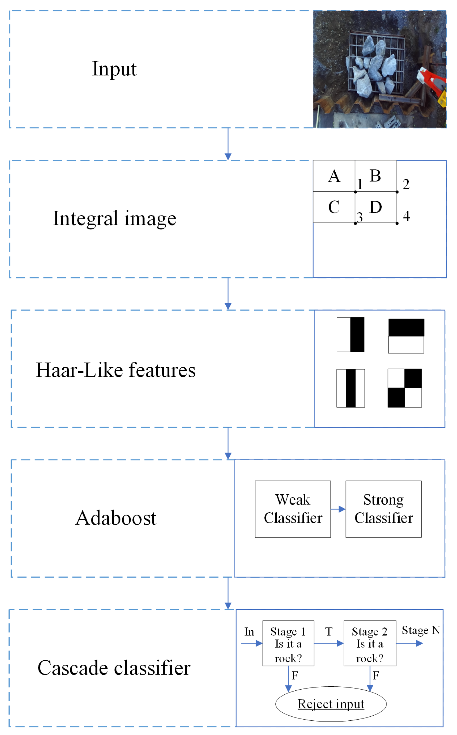
2.1. Viola-Jones Algorithm

The Viola-Jones algorithm was developed in 2001 to detect facial features. This algorithm incorporates several contributions, such as the integral image, construction of a robust classifier through weak classifiers using AdaBoost, and successful development of a method to combine classifiers in a cascade structure. This cascade structure increased the speed of the detector by focusing on the most critical regions of the image. Figure 1 shows the Viola-Jones algorithm.

The integral image was designed to accelerate the process of calculating the Haar-like features. The value at any point $(x,y)$ in the integral image is the sum of all pixels in the input image that are above and to the left of $(x,y)$. The sum of all pixels within rectangle D of Figure 1 can be calculated using four numbers mentioned as [1, 2, 3, 4]. AdaBoost is used to construct a robust classifier by assigning weights to the most relevant features. Finally, the classifiers were introduced in a cascade to pay more attention to the windows that present the target and less attention to those that contain the background.

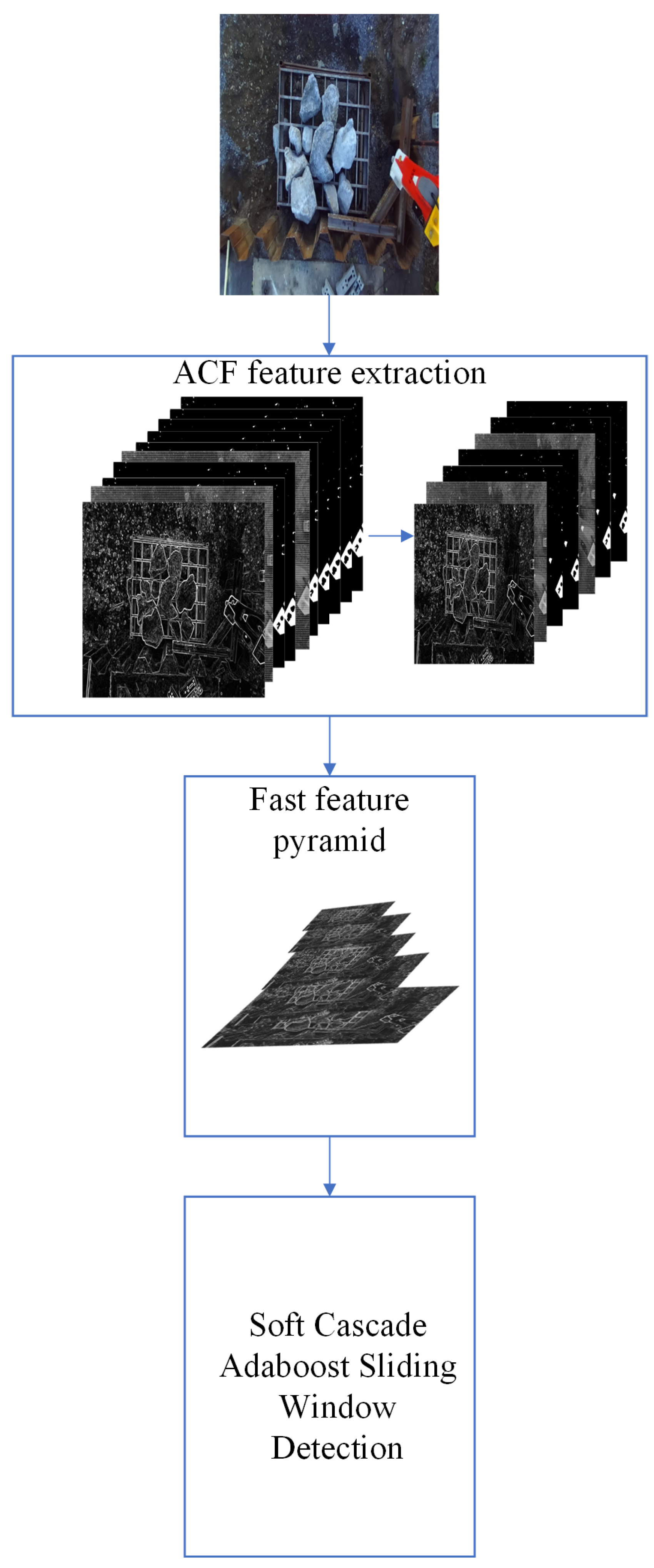
2.2. ACF Algorithm

One of the goals of the ACF detector is to achieve a rich representation of the image without high computational cost. The fractal features of images allow reliable prediction of their structures across scales. Figure 2 shows the ACF algorithm.

In the first stage, features such as the LUV color space, gradient magnitude, and HOG are extracted from input image I. The results were then smoothed to obtain low-resolution channels (aggregations). In the second stage, a multi-scale feature pyramid is constructed. To achieve this, image I is resized to scale s. Subsequently, linear and non-linear transformations ($\Omega$) are applied to the resized image I. Equation (1) shows the steps in the second stage.

$$C_s=\Omega \left(I_s\right)=\Omega \left(R(I,s)\right),$$

(1)

where C_s is the feature channel at scale s, $\Omega$ represents linear and non-linear transformations, and R is the resampling function. In the third stage, AdaBoost is used to train and combine the decision trees on the features. Subsequently, a multi-scale sliding window was applied for detection.

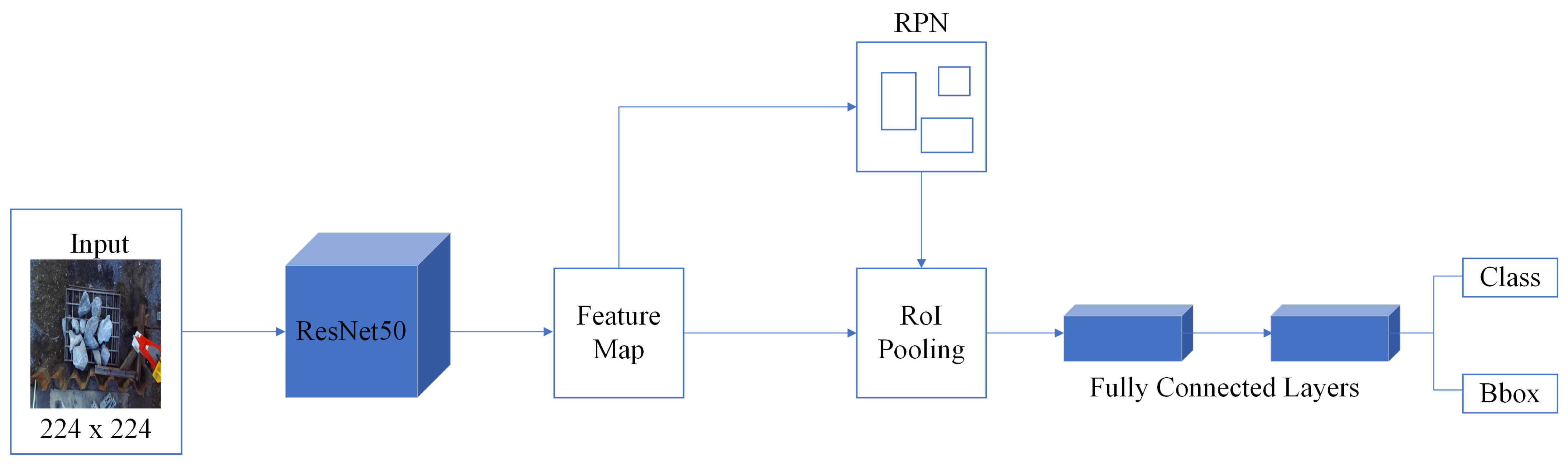
2.3. Faster R-CNN

One deep learning approach utilizes regions with convolutional networks. This method integrates rectangular region proposals with features derived from Convolutional Neural Networks (CNNs). This approach functioned as a two-stage detection algorithm. In the initial stage, a subset of regions likely to contain the object of interest is identified. Subsequently, the object within each proposed region was classified in the second stage. Models based on these algorithms typically consist of three phases:

• The detection of regions in the image that may contain an object, referred to as the proposed regions.
• Extraction of CNN features from the proposed regions.
• Classification of objects using the extracted features.

In these algorithms, the three variants are R-CNN, Fast R-CNN, and Faster R-CNN. Each variant attempts to optimize, accelerate, or improve the results of one or more phases. Figure 3 shows the structure of the Faster R-CNN network used in this study.

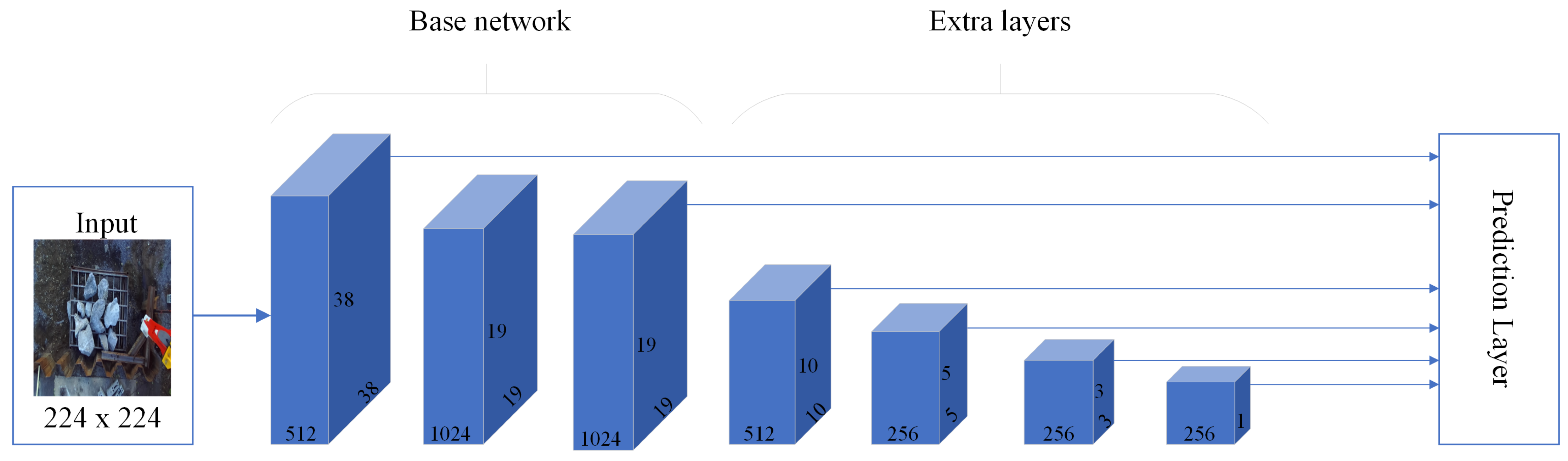
2.4. SSD Algorithm

The SSD algorithm utilizes a single-stage detection network that merges the predicted detections from the multi-scale features. This algorithm outperforms two-stage algorithms, such as Faster R-CNN, in terms of speed and offers higher accuracy than specific one-stage algorithms, such as YOLO v2. Figure 4 shows the SSD algorithm. The detector obtains a prediction network across multiple feature maps that are derived by passing an image through a CNN. Subsequently, the detector combines and decodes the predictions to generate bounding boxes. The network leveraged the bounding box size to determine the class of the object under analysis. For each bounding box width, the SSD predicts the following attributes:

• Box width offsets. This refines the position of the width of the box.
• Class probability. It predicts the assigned class label for each bounding box width.

2.5. YOLO v4 Algorithm

YOLO is a deep learning algorithm that has been widely used for object detection since its publication in 2015. To date, eight versions have been developed. The core of YOLO consists of a small-sized and computationally efficient model, making it suitable for object detection in videos. YOLO v4 introduced significant changes compared to previous versions, focusing on substantial improvement and data comparison. 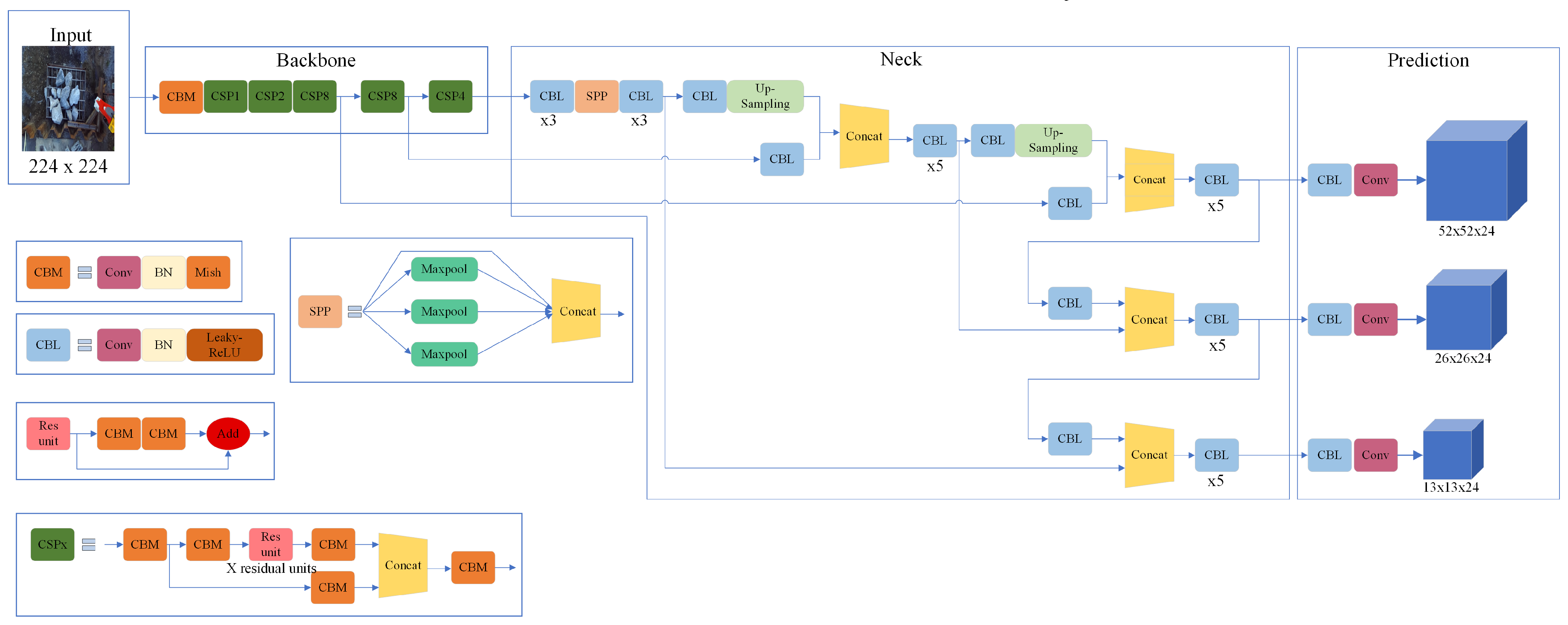Figure 5 shows the structure of the YOLO v4 network used in this study.

The main contributions of YOLO v4 are as follows:

• An efficient and powerful model that enables fast and accurate detector training is proposed.
• During detector training, methods such as bag-of-freebies and bag-of-specials were verified.
• It includes methods that make it more efficient and useful for training on a single GPU, such as Cross-Iteration Batch Normalization (CBN) and the Self-Attention Method (SAM).

The backbone is usually a pre-trained CNN. This backbone acts as a feature extractor for the input image. The neck connects the backbone and head. It consists of a Spatial Pyramid Pooling (SPP) module and Path Aggregation Network (PAN). In the SPP module, the features are convolved three times and then maximally pooled with maximum pooling layers of different sizes. The pooled results were concatenated first and then convolved thrice. PAN performs convolution between the feature extraction layers and SPP. This module reuses information from lower-level layers in higher-level layers through connections or inverse paths, thereby allowing the detection of objects of different sizes. YOLO v3 was used in the prediction module, where the class probabilities, object confidence, and bounding box width and height were predicted.

2.6. Backbones

Backbones are usually part of the networks responsible for extracting features from images. CNNs are often pre-trained on large databases. These backbones allow leveraging of the learned features as a starting point for a particular task. In this research, several backbones were evaluated in Faster R-CNN, SSD, and YOLO v4 architectures. The residual Network (ResNet) [33] is a CNN, and among the most well-known variants are ResNet-50 and ResNet-101. 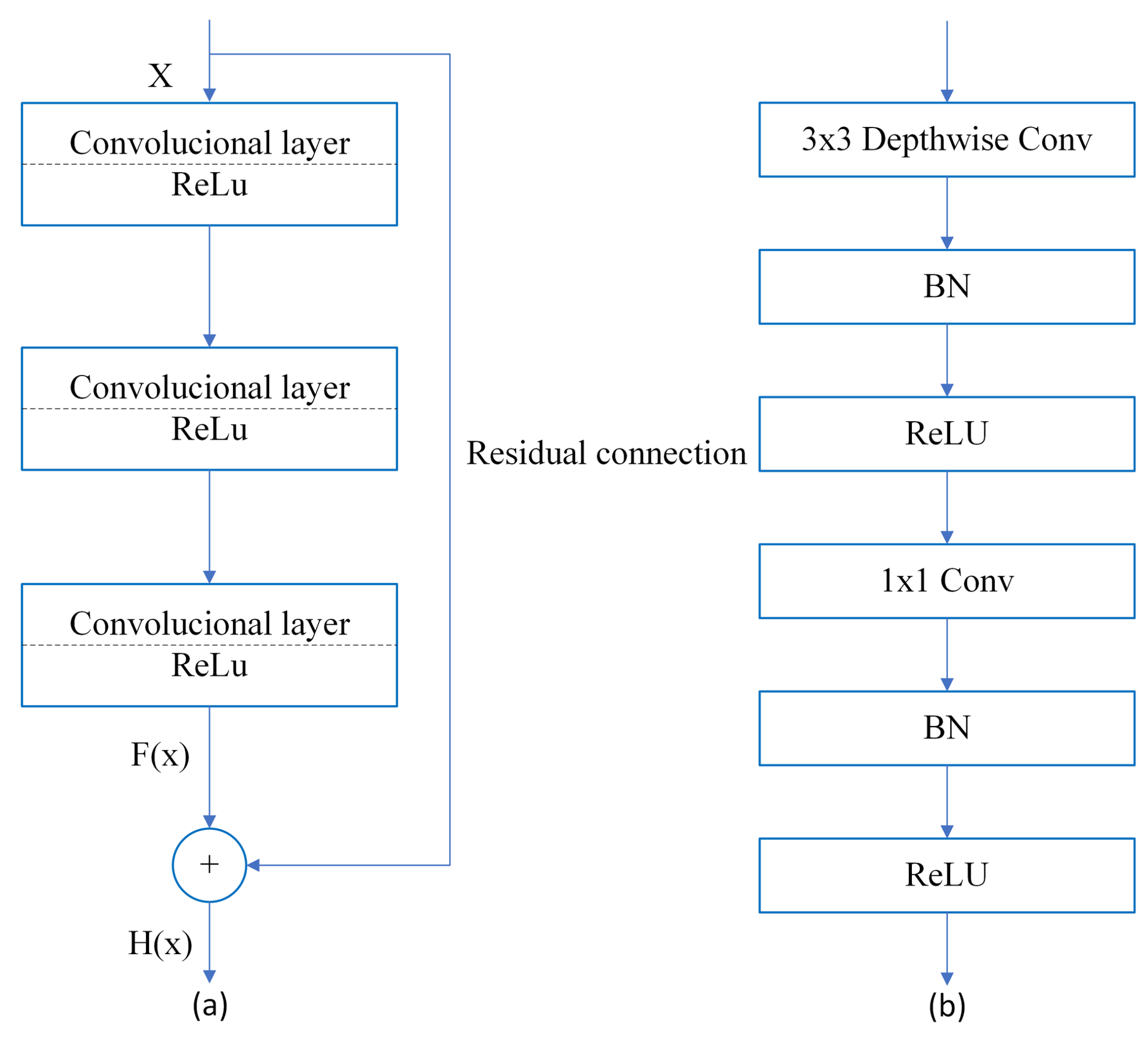ResNet was trained with over a million images from 1000 categories in the ImageNet database [34]. The size of the input image was 224 × 224 px. ResNet was designed to mitigate the problem of vanishing gradients that occur as network depth increases. To achieve this, residual connections are introduced, as shown in Figure 6a. These residual connections allow input X to skip the convolutional layers and be added to the output of those layers, $F\left(x\right)$. MobileNets [35] is designed for use in embedded and mobile applications.

MobileNet was trained using the ImageNet database. This network introduces two hyperparameters that allow for low latency, while maintaining adequate accuracy. Figure 6b illustrates these hyperparameters. First, it transforms the standard convolution into a 3 × 3 depthwise convolution through factorization. Then, it performs pointwise convolution using a 1 × 1 convolution. The introduction of these parameters primarily aims to reduce the model size and computational cost. The combination of these layers is known as depthwise separable convolution (DSC). MobileNetv2 [36] has a structure that is very similar to that of MobileNet. It utilizes the layers mentioned above; however, in a different manner, the input is transformed with a pointwise convolution layer to expand the channels. It passes through a 3 × 3 depthwise convolution to decrease the computational complexity. It passes through another pointwise convolution layer. These steps form the basic unit of MobileNetv2, which is called at the residual bottleneck block.

YOLO v4 uses CSPDarkNet53 [32] as its backbone. This was derived from the DarkNet53 backbone of YOLO v3 [37]. It was trained on the Common Objects in Context (MS COCO) database [38], which contains over 200,000 labeled images with approximately 1.5 million instances of objects in 80 categories. The input image size was 416 × 416 px. The addition of cross-stage connections (CSP) allows the integration of feature maps from the initial to the final stage. The main goal is to achieve a rich combination of gradient while reducing computational costs. CSP reduced the computational cost by approximately 20%.

3. Experiment Setup and Evaluation

In this section, we address the tools and database used, metrics for algorithm evaluation, configuration of these algorithms, and evaluation results.

3.1. Tools

MATLAB ® version R2022a was used to train and test the models on a laptop with the following specifications: Intel-Core i7-11800H CPU @ 64-bit 2.30 GHz, 16 GB RAM, NVIDIA GeForce RTX 3060, and CUDA v11.7.

3.2. Dataset

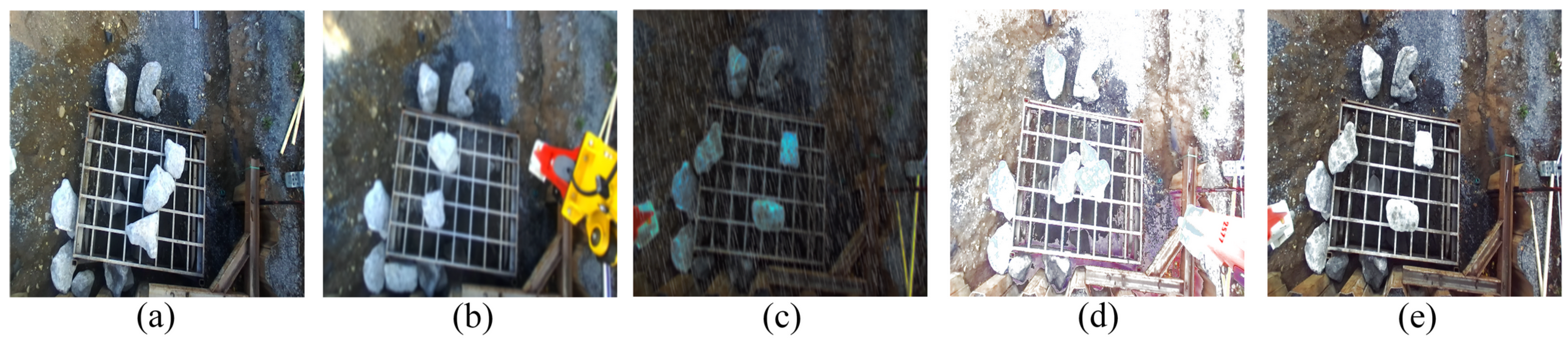
In this study, we used the database reported in [25]. It has 23,850 images with a size of 1280 × 720 px. The number of rocks in a scene can vary between one and fifteen. The primary motivation for using this database is the presence of several scenes with visual contamination. This contamination represents a challenge for machine learning algorithms, in addition to being present in natural mining environments. Figure 7 shows the database used in this study.

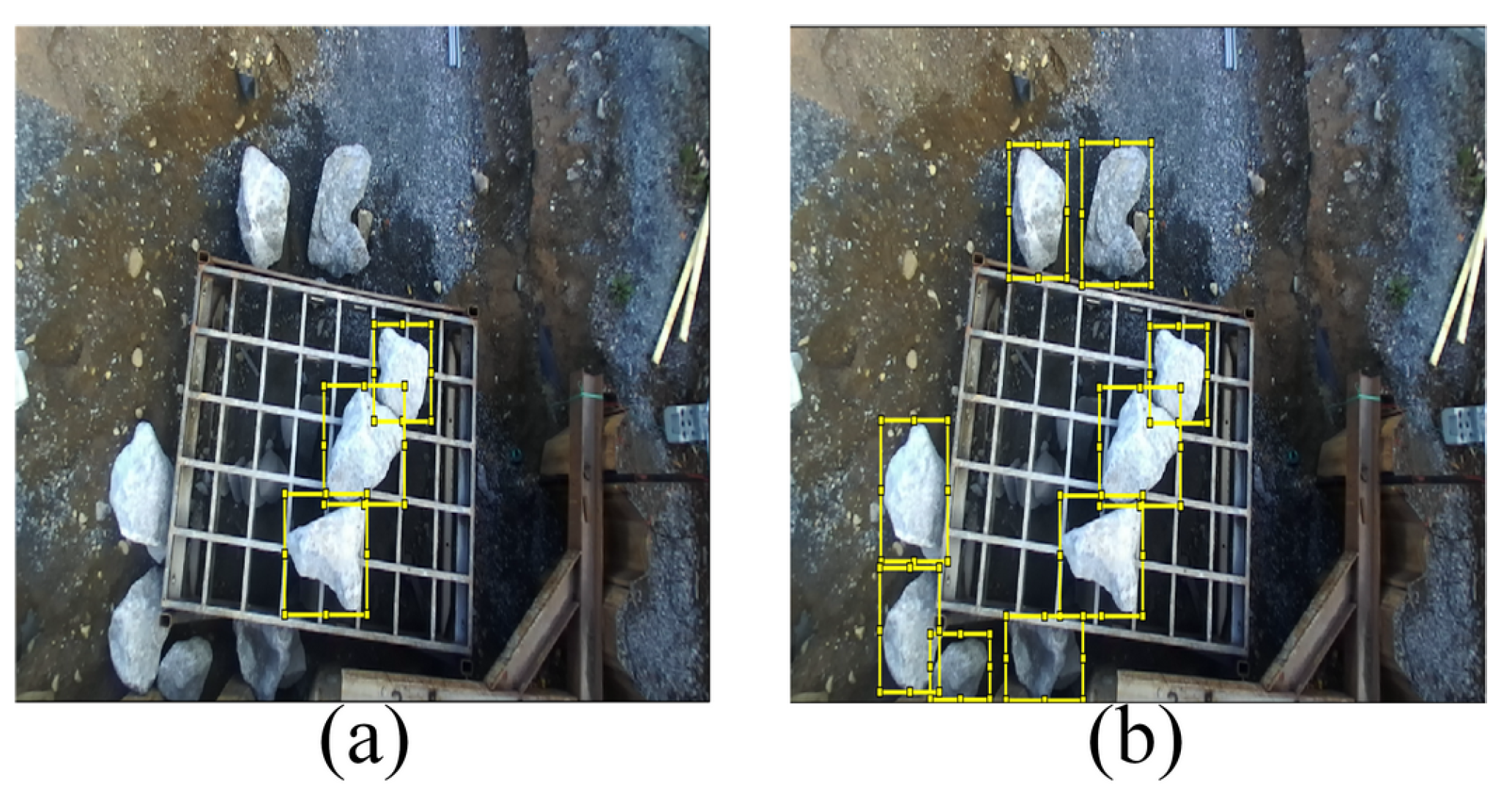
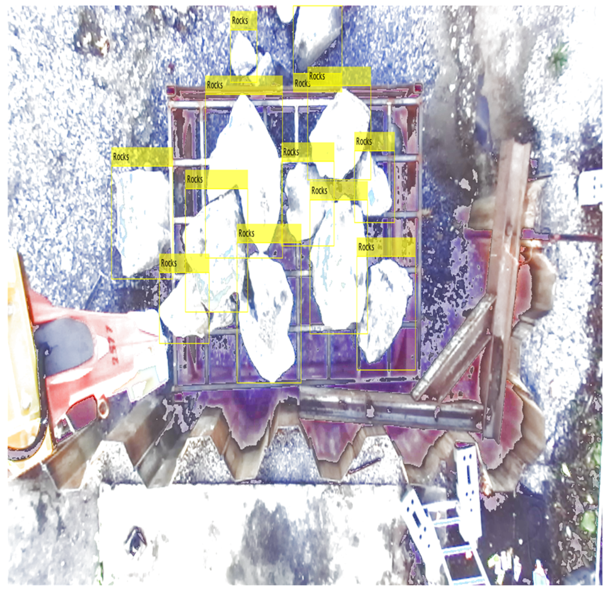
The labeling in this database has some drawbacks; for example, Figure 8a shows that they only label the rocks on the grid. This is undesirable since, in many mines, rocks are on the ground, and it can also positively affect the performance of detectors. All rocks in each scene were labeled using the MATLAB® version R2022a Image Labeler App, as shown in Figure 8b. We randomly selected 200 images for each visual contamination category. We marked 1000 images with 9460 Regions of Interest (ROIs). We selected 80% (7565 ROIs) for training, 10% (928 ROIs) for validation, and 10% (967 ROIs) for testing.

3.3. Performance Metrics

To evaluate and validate the algorithms, we used the following metrics: precision (P), recall (R), $F_1$-score, and average precision ($AP$). These metrics are commonly used in research studies [39,40,41] to analyze the performance of models. The precision, recall, and $F_1$-score are defined by Equations (2)–(4).

$$P=TP/(TP+FP),$$

(2)

$$R=TP/(TP+FN),$$

(3)

$$F_1=2\times (P\times R)/(P+R),$$

(4)

where $TP$, $FP$, and $FN$ represent the true positives, false positives, and false negatives, respectively. $AP$ is the area under the precision–recall curve. This measure describes the overall performance of the model across the different confidence thresholds. The $AP$ is defined in Equation (5).

$$AP=\sum _n\left((r_{n+1}-r_n)·p_{\mathrm{interp}}\left(r_{n+1}\right)\right),$$

(5)

where $p_{\mathrm{interp}}\left(r_{n+1}\right)={max}_{\tilde{r}\ge r_{n+1}}p\left(\tilde{r}\right)$. The precision value at a specific recall value is denoted by $p\left(\tilde{r}\right)$.The $AP$ values ranged between 0 and 1 based on a specific Intersection over Union (IoU). In this case, IoU was 0.5.

3.4. Algorithm Configuration

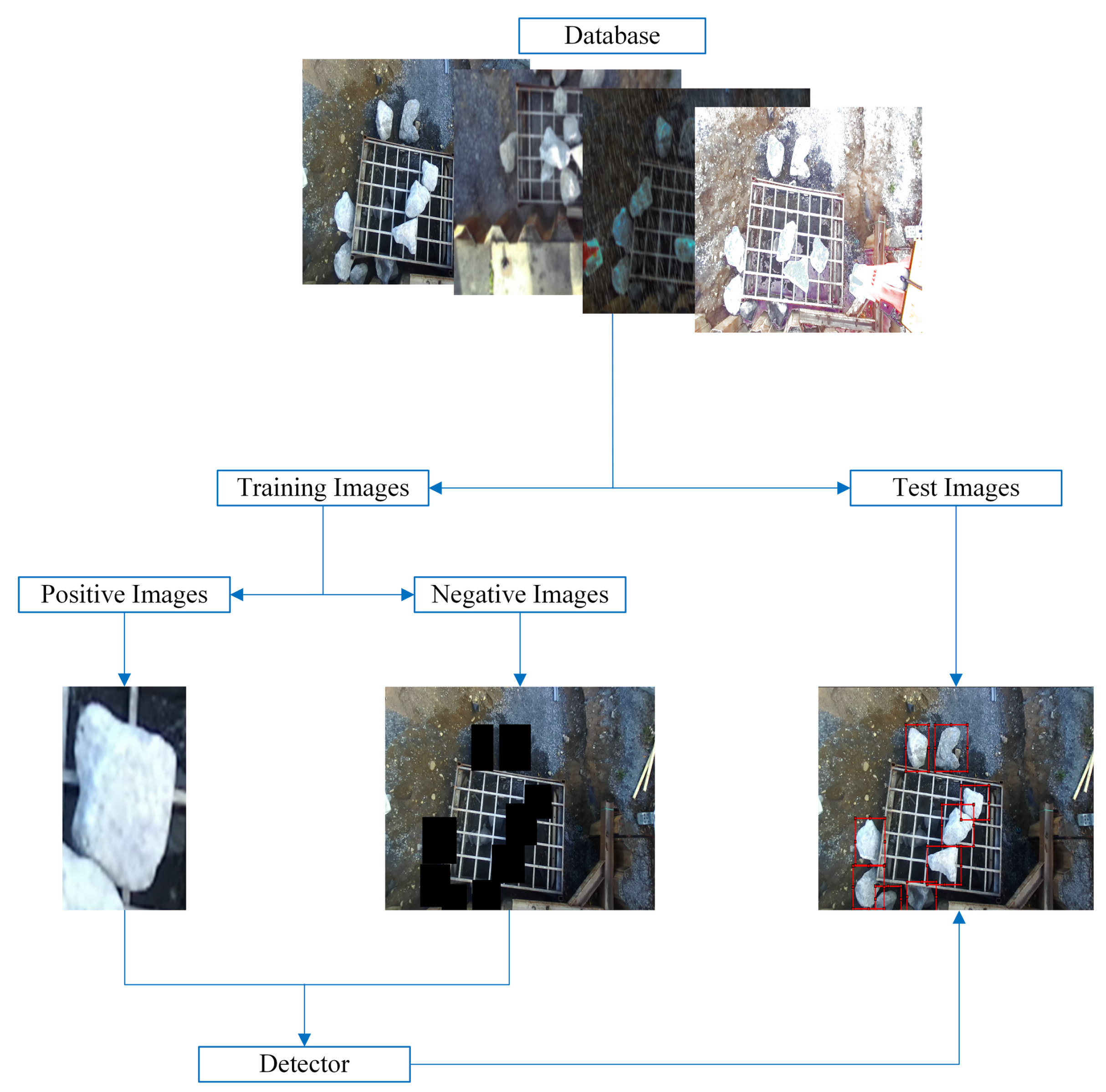
Machine learning algorithms require parameter settings for training. Various features, such as Haar-like, local binary patterns (LBPs), and HOG, can be used in the Viola-Jones detector. In this study, the detector is trained using these features. The ROI size was automatically calculated as 32 × 32 px. The methodology followed in this study to train and test the detector is shown in Figure 9.

To create negative images, scenes that did not contain an ROI were selected. The ROIs were then extracted from the positive images and used to generate 360,000 negative images through 360° rotations. The NumCascadeStages and FalseAlarmRate parameters were crucial to the process, and were set to 10 and 0.01, respectively. Although decreasing the FalseAlarmRate or increasing the NumCascadeStages can improve the robustness of the detector, it significantly lengthens the training time. For this study, it took approximately 60 h to train the Haar-like feature, whereas LBP and HOG features took 10 h and 20 h. All other parameters were set to their default values.

Several experiments were performed on an ACF detector with 10 stages each. The modified parameters were the number of weak classifiers and the ROI size. In the first experiment, these parameters were not modified, that is, the ROI was 23 × 23 px, and the number of weak classifiers was 2048 in all stages. In the other experiments, variations were made in these parameters to analyze their influence on the final detector. The ROI used in the combinations was 52 × 52 px, and the weak classifiers were [256 256 512 512 1024 1024 2048 2048 4096 4096]. This ROI was obtained from the maximum anchor box size of the deep learning algorithms. The experimental details are presented in

Table 1. Experiments with the ACF algorithm.

Parameters	Exp-1	Exp-2	Exp-3	Exp-4
Epochs	10	10	10	10
ROI	23 × 23	23 × 23	52 × 52	52 × 52
Weak classifiers	2048	Var	2048	Var

.

In this case, the negative images were automatically generated by the algorithm. The remaining parameters were set to default values. The total training time ranged from 0.15 to 0.20 h.

In the case of detectors based on deep learning, images were resized to 224 × 224 px. The anchor boxes were then estimated. According to this database, the obtained anchor boxes were [52 26; 42 28; 47 21; 34 25; 38 19; 26 24; 29 16; 22 15; 34 8]. A CSPDarkNet53 backbone was used in the YOLO v4 detector. ResNet-50 and MobileNetV2 were used as backbones for the Faster R-CNN and SSD detectors. The selection of these backbones was justified by the good results presented in [43,44,45,46]. The training times for the detectors were 2.25 h and 0.25 h.

3.5. Hyperparameters

Properly selecting parameters is a challenging task, especially for deep learning algorithms. This research aimed not to find the optimal parameters for each algorithm but to identify a potential candidate for use in challenging mining tasks. In the case of the Viola-Jones algorithm, the selection of the learning rate and the number of cascades was directly related to the training time. Decreasing the learning rate increased the training time without substantially improving the algorithm’s accuracy. This effect was compounded when using the Haar-like feature in the detector’s training. For the ACF algorithm, the main modifications were directly related to the ROI and the number of weak classifiers. The ROI size was obtained from the mean sizes of the training bounding boxes, and the number of weak classifiers was varied to assess its impact on the results.

A straightforward guide must be used to select the appropriate parameters in the deep learning-based detectors. However, specifically for rock detection, the optimizer that yielded the best results was Adaptive Moment Estimation (ADAM), although it does not imply it will always be the case. This method offers very good results and has been used in several investigations [47,48]. Batch size selection is related to the computational power available for loading images, depending on the machine’s hardware used for training. The learning rate is the most crucial parameter in training, chosen primarily to avoid significantly altering neuron weights during the stages. This decision was made because pre-trained backbones from other datasets were used as the basis for training. Moreover, similar configurations have been used in other research studies [14,15,16,17]. The number of epochs was chosen to be the same across all algorithms. The hyperparameters that were used are listed in

Table 2. Hyperparameters of the ADAM optimizer.

Hyperparameters	ADAM
Epochs	10
Batch size	8
Learning rate	0.001
Weight decay	0.0001
Gradient decay	0.9
Squared gradient decay	0.999

.

3.6. Results of Rock Detection

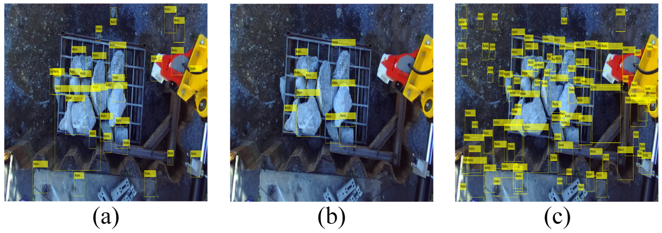
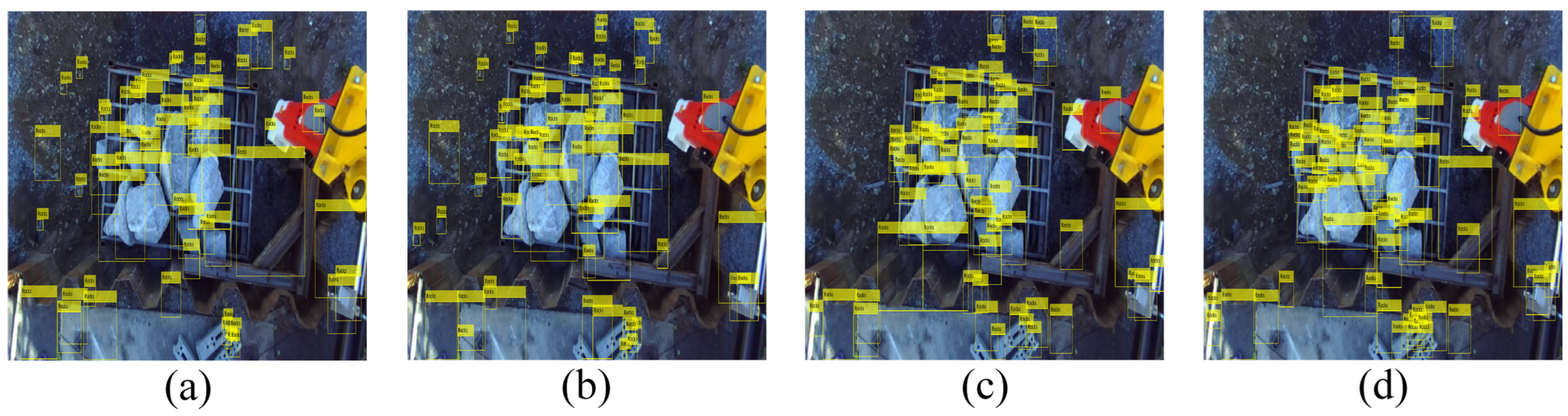
Figure 10 shows the results of the Viola-Jones algorithm against the different types of features used. It is observed that the Haar-like and HOG features present many FPs; however, the LBP feature effectively identifies the rock characteristics. Figure 11 shows the results of the ACF algorithm before the different experiments were conducted. Similar to the Viola-Jones algorithm, many false positives were observed for all variants.

Figure 12 and Figure 13 show the results of rock detection in a test image from the database and in an image that does not belong to the database. This was done to analyze the generalization capacity of these algorithms for images with different characteristics from the training images. The size of the images that were not from the database was 3264 × 2448 px. These two images correspond to a normal scenario without visual pollution. It is observed that the algorithms manage to detect rocks, but they have the problem of presenting many false positives, except for YOLO v4. The YOLO v4 algorithm effectively detects rocks even in images that do not belong to the database, and this demonstrates the generalization capacity obtained.

3.7. Results of Evaluated Metrics

In this section, the results of the machine learning algorithms are analyzed with respect to P, R, $F_1$-score, $A{P}_{50}$, and average detection time.

Table 3. Metrics of detectors.

Algorithm			Metrics (%)
		$\mathit{P}$	$\mathit{R}$	${\mathit{F}}_{\mathbf{1}}$-Score
Viola-Jones	Haar-like	40	100	57.1
	LBP	82.2	85	83.5
	HOG	10	100	18.1
ACF	Exp-1	54	75.7	63.1
	Exp-2	44.7	77.8	63.1
	Exp-3	41.8	78.6	54.6
	Exp-4	39.8	78.2	52.7
Faster R-CNN		97	93	94.9
SSD		99.6	90	94.5
YOLO v4		99.9	99.7	99.8

show the P, R, and $F_1$-score results of the Viola-Jones, ACF, and deep learning detectors.

The results shown by these algorithms concerning precision are mainly due to the presence of $FP$. Their authors have debated this large number of $FP$ as a disadvantage, because they detect the same object multiple times. Multiple detections occurred because of the use of sliding windows at different scales. The Haar-like and HOG features generally performed worse than the LBP features. The increase in the ROIs and number of weak classifiers in the ACF algorithm did not yield good results concerning precision; however, a slight increase in recall was observed. The LBP feature in the Viola-Jones algorithm showed the best results for all metrics compared to the analyzed classic algorithms. This feature efficiently describes the characteristics of the object of interest. These algorithms require a post-processing stage to decrease $FP$ and thus increase the precision.

In general, deep learning algorithms achieve better results than classic algorithms. This was expected because of their excellent generalization capabilities. In these detectors, different types of networks, such as ResNet-50, MobileNetV2, and CSPDarkNet53, are used as backbones. The Faster R-CNN algorithm achieved the lowest precision value owing to the presence of $FP$. These algorithms have fewer FPs than the classic algorithms owing to the Non-Maximum Suppression (NMS) technique. This technique helps eliminate redundancy and reduce the number of overlapping bounding boxes. The SSD algorithm produced the worst results in terms of recall, which might have been influenced by using MobileNetV2 as a backbone. The YOLO v4 algorithm displayed excellent precision, recall, and $F_1$-score results.

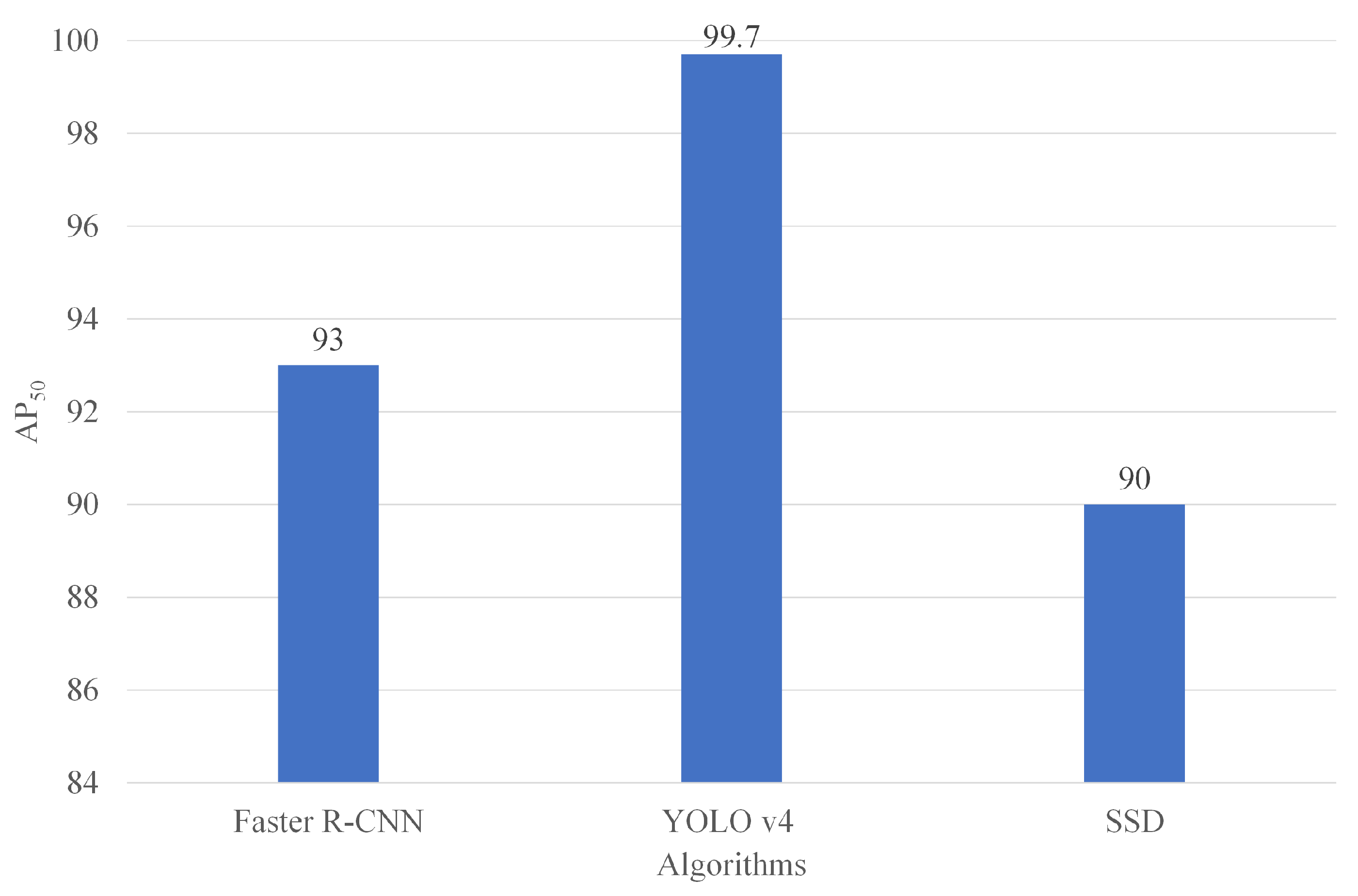
The $A{P}_{50}$ metric is widely used to evaluate object detection algorithms. This study used this metric in deep learning algorithms because they achieved the best results for P, R, and $F_1$-score. Figure 14 shows the $A{P}_{50}$. The $AP$ provides a single performance metric that summarizes the shape of the precision–recall curve. All deep learning algorithms achieved an $A{P}_{50}$ above 89%, with YOLO v4 achieving the highest value at 99.7%. This metric is important because it shows the average precision of the model when the recall is 50%.

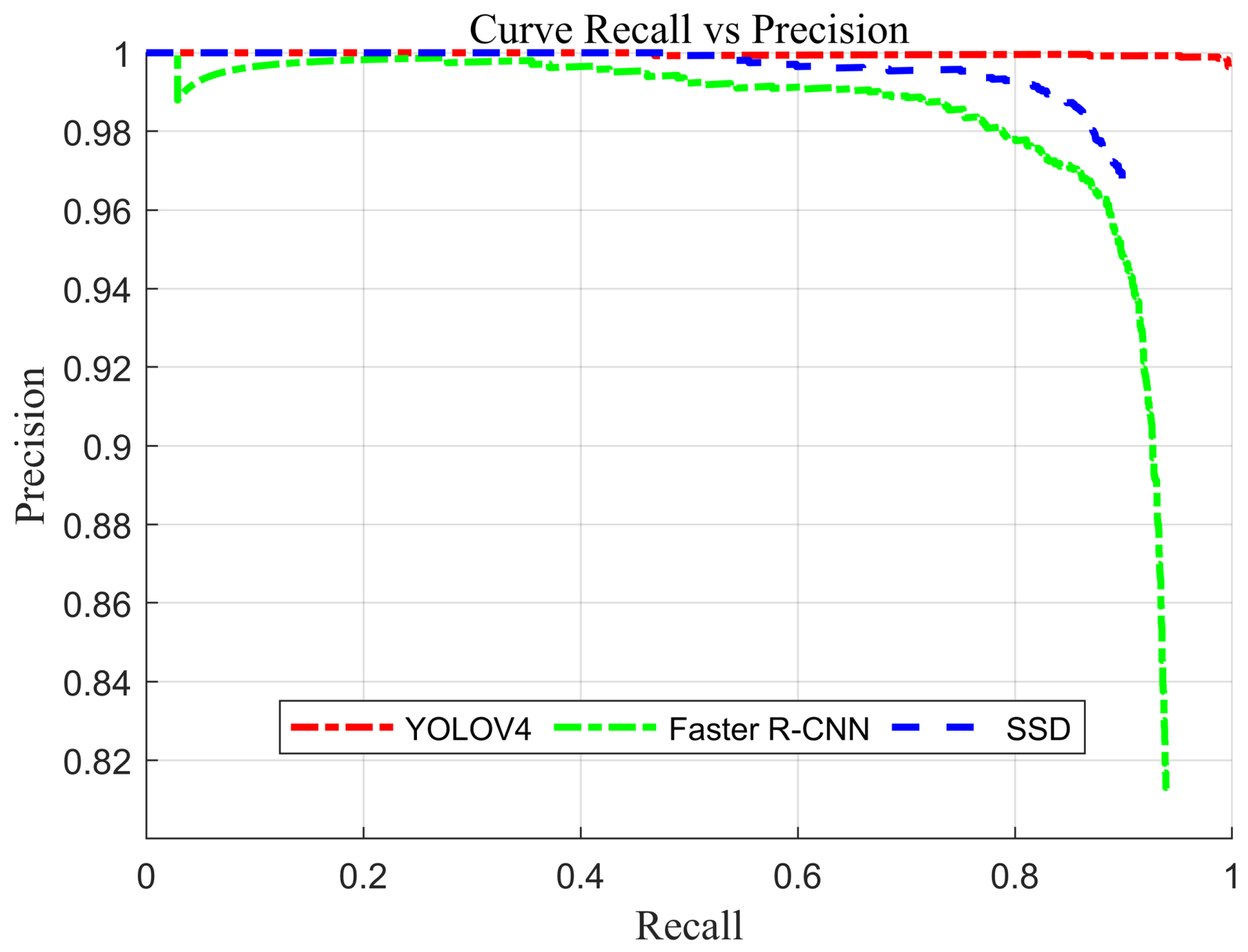
Figure 15 shows the precision vs. recall curve for the deep learning algorithms under analysis. This curve is a valuable tool for understanding the performance of the trained classification models. It also offers insight into how the performance of the models fluctuates across different thresholds. Given these factors, it is apparent that the YOLO v4 algorithm outperforms the other algorithms.

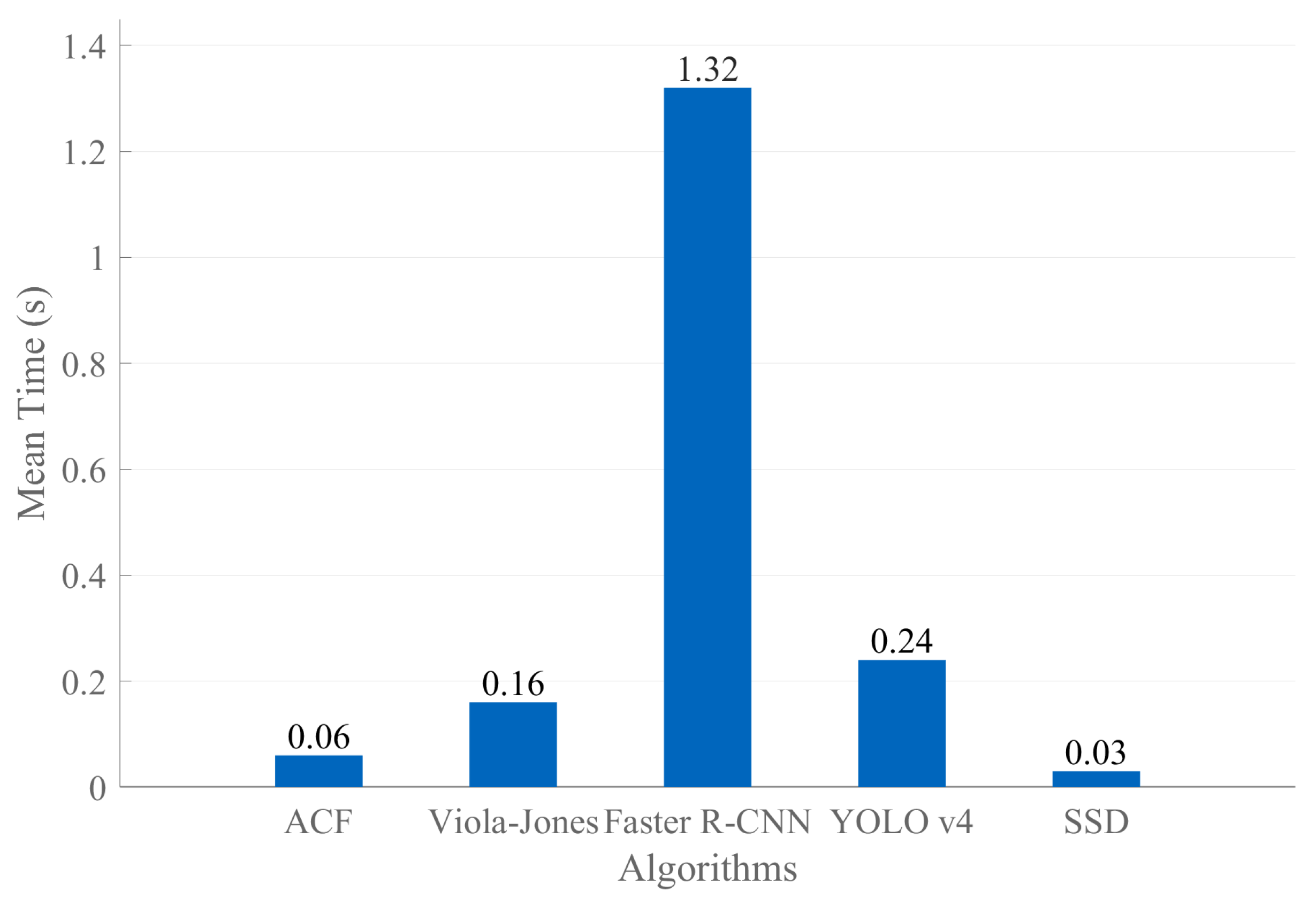
The detection time of an algorithm is a crucial parameter when it is used in real-time applications. In this regard, we tested the previously mentioned algorithms to assess their detection speed. We conducted 50 runs for each test image and calculated the average detection time. Figure 16 shows the average number of detections.

As a result, the fastest algorithm is SSD, with an average of 0.025 s, and the slowest is Faster R-CNN, with an average of 1.32 s. The latter is expected because one-stage deep learning methods are faster than two-stage methods. All algorithm times were low, enabling them to be used in real-time applications. The speed of the SSD algorithm is mainly attributed to using a lightweight network like MobileNetv2. Its main advantage is that it can be employed in embedded systems, which is common in practical applications in mining environments. Although it is less accurate than other analyzed deep learning algorithms, we could improve it by incorporating attention modules.

3.8. Influence of Visual Contamination on the Analyzed Algorithms

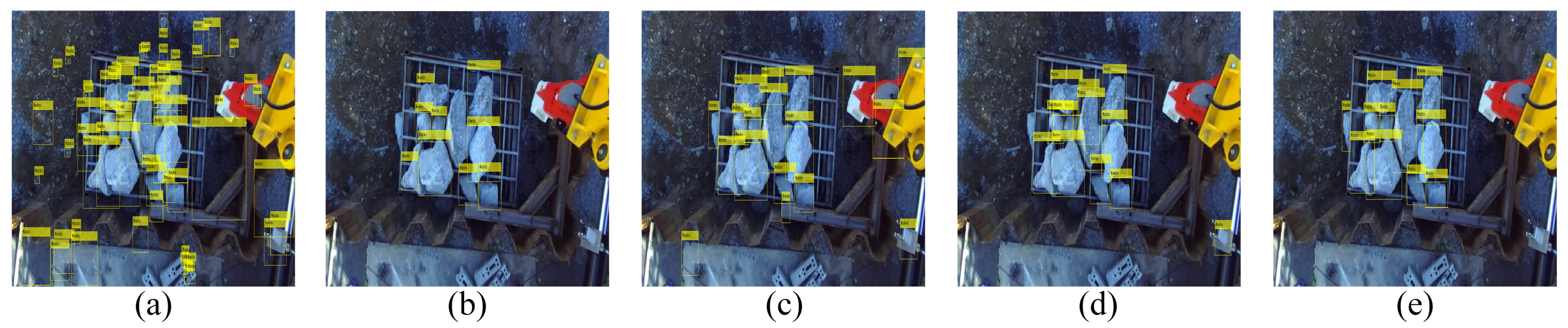
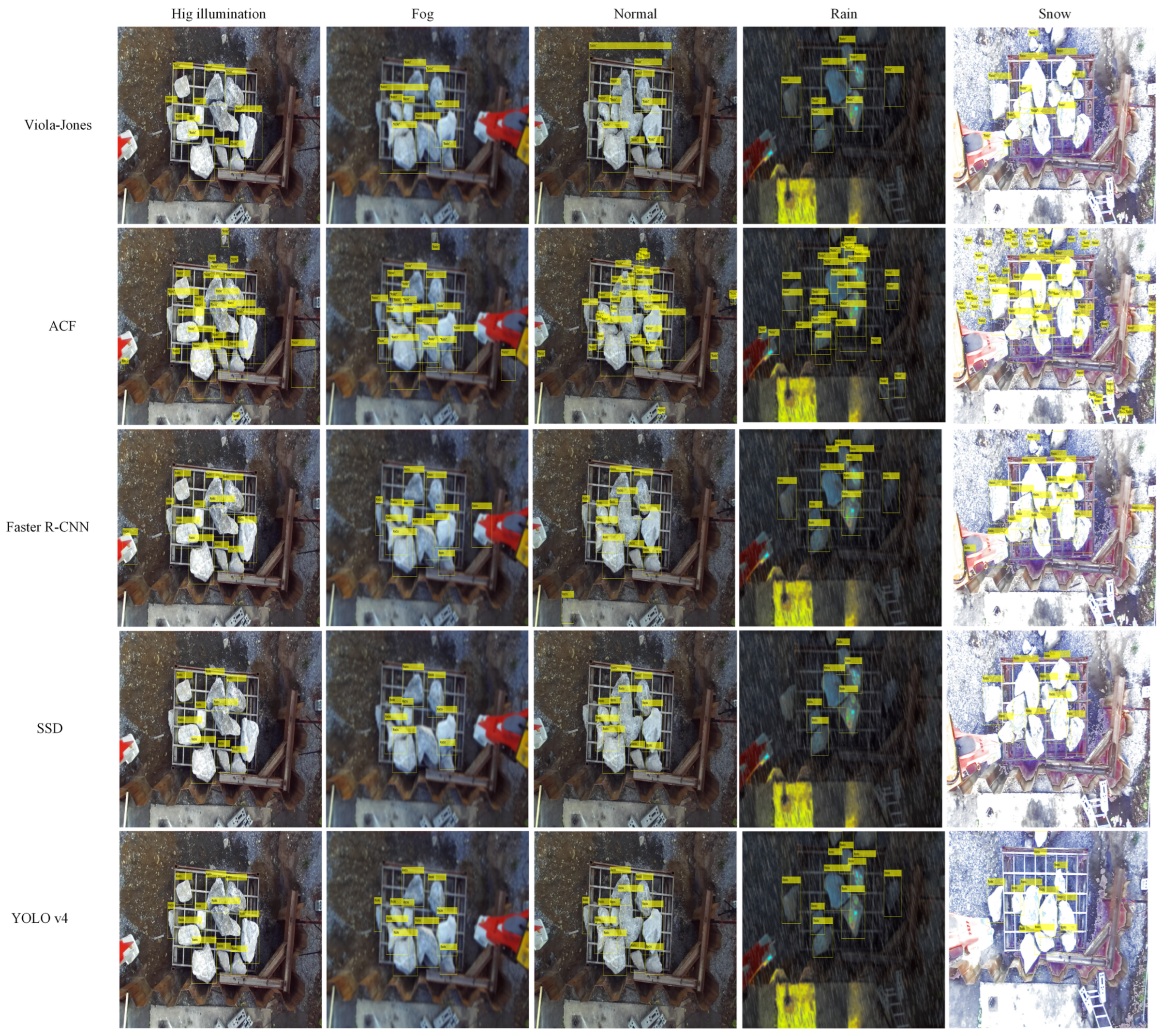
Figure 17 illustrates rock detection in various evaluated scenarios of visual contamination. The presented machine learning algorithms exhibit superior results compared to their variants. The ACF algorithm showed a significant number of FPs. It was observed that visual contamination from snow resulted in the highest number of FPs, followed by rain, while others maintained relatively similar amounts of FPs. Regarding the Viola-Jones algorithm, few FPs were observed in the LBP feature, demonstrating its efficiency in capturing rock characteristics across all scenarios. In the normal scenario, FP occurrences were observed at larger scales due to the processing performed by the algorithm, which utilizes a sliding window at multiple scales.

Regarding deep learning algorithms, all showed promising results; however, YOLO v4 demonstrated excellent performance. The Faster R-CNN algorithm exhibited FP occurrences, while the SSD algorithm had no FPs but failed to detect some objects. In all cases, the YOLO v4 algorithm correctly detected rocks. Figure 18 illustrates a case where the YOLO v4 algorithm fails to detect one rock, primarily due to the absence of a well-defined boundary between two rocks and their overlapping level. The scenarios that most affected the algorithms overall were snowy and rainy conditions.

3.9. Some Benefits and Limitations of Deep Learning vs. Machine Learning Algorithms

Deep learning algorithms have come to revolutionize multiple areas, primarily due to the efficiency they provide. However, they are still represented as black boxes and in-depth studies are needed to explain their functioning thoroughly. Among the main advantages of deep learning algorithms is a considerable increase in efficiency across various evaluation metrics compared to classical algorithms. This has led to widespread use in crucial areas such as medicine, industry, agriculture, autonomous driving, and robotics.

The utilization of CNNs eliminates the need for the feature engineering phase, which is customary and essential in classical algorithms. This phase involves selecting and normalizing features, among other procedures. Additionally, they can adapt to various conditions through parameter tuning, flexibility not achievable in classical algorithms. The primary disadvantage of these networks is the need for more understanding of their internal workings and the requirement for a large amount of labeled data for proper performance.

On the other hand, classical algorithms provide a better understanding of their internal workings, and some require a smaller amount of labeled data. However, they generally exhibit lower overall performance.

In the context of rock detection in visually contaminated mining environments, YOLO v4 has implemented substantial improvements in various areas, including:

• Efficient backbone with CSPDarknet53. Incorporates CSPDarknet53, an enhanced version of Darknet, using the CSP concept to improve feature learning efficiency. This results in a more adequate representation of visual features, which is particularly beneficial in visually complex mining environments.
• PANet as Head. YOLO v4 uses this module to enhance information integration at different spatial scales. This is crucial in rock detection, as there can be significant variations in the size and shape of rocks in mining environments. PANet helps handle these variabilities, improving the model’s ability to detect objects at different scales.
• Hyperparameter optimization. Enables hyperparameter optimization, including grid size and anchor dimensions. Adjusting these parameters for rock features and mining environments improves the model’s accuracy.
• Improvements in post-processing. YOLO v4 has enhanced post-processing to reduce false positives and improve accuracy. For example, it uses an improved NMS to eliminate redundant detections. It has improved model stability, influencing the mitigation of issues such as oscillations in predictions or unstable behaviors in certain scenarios. It offers the ability to adjust specific post-processing parameters, such as thresholds and suppression criteria, providing flexibility to adapt the model to different conditions and application requirements.

4. Conclusions and Future Work

The various complexities in images render object detection and classification a continuously developing area. In mining operations, fog, snow, and suspended particles can interfere with the detection of objects, such as rocks. Therefore, any machine learning algorithm used in these operations must meet specific requirements such as acceptable speed, adequate recall, and precision. This study evaluated various machine learning algorithms used for object detection.

Training algorithms in both machine learning and deep learning is a challenging task. Fundamental limitations or challenges include the selection of training parameters, manual database labeling, hardware requirements, primarily for deep learning algorithms, the proper selection of metrics, and the evaluation function. Additionally, difficulties were encountered in the training quality of deep learning algorithms when different versions of CUDA were installed, which was resolved by installing the required version according to the installed GPU. Challenges were identified in developing SSD and Faster R-CNN detectors regarding the selection of layers to build the detection network, leading to potential areas for future research.

The Viola-Jones and ACF algorithms showed the lowest precision, recall, and $F_1$-score results. The low precision of these algorithms is primarily due to the occurrence of FPs, which their authors address as a present inconvenience. The local binary patterns (LBP) feature efficiently encoded the rock characteristics compared to Haar-like and histogram of oriented gradients (HOG) features. The ACF algorithm improved the recall when the number of weak classifiers was varied, but the precision decreased. The low detection time of these algorithms enables their real-time use. A post-processing stage, such as Non-Maximum Suppression (NMS), could increase the evaluated metrics.

In general, algorithms based on deep learning achieved the best results in terms of precision, recall, $F_1$-score, and $A{P}_{50}$. This is expected owing to their significant improvements in machine learning. The increase in the training data was not used in these algorithms to make a proper comparison with the classic algorithms. The YOLO v4 detector with the CSPDarkNet53 backbone achieved the best results in the metrics evaluated compared with the SSD and Faster R-CNN architectures. The detection times were generally comparable to those obtained through the Viola-Jones and ACF algorithms, except for the Faster R-CNN detector, which had an average time of more than 1 s. The increase or decrease in these times depends on the architecture used and the backbone network, among other parameters.

Regarding the $A{P}_{50}$ metric, all the deep learning algorithms surpassed 90%, with the YOLO v4 detector achieving the best results. Generally, YOLO v4 has been proposed as a candidate for use in mining environments with visual pollution.

Future lines of research, including improvements in the analyzed algorithms, especially those related to deep learning, are being considered. Variations in the backbones, including attention mechanisms, could be explored. Additionally, an algorithm is currently being developed to reduce false positives. We appreciate the significance of this aspect in validating the functionality of the analyzed algorithms. The experimentation with hardware is indeed part of our planned next stage of research. Currently, we are actively engaged in the process of applying for research projects to secure funding for the acquisition of the necessary hardware.