Article

Prediction of Traffic Incident Locations with a Geohash-Based Model Using Machine Learning Algorithms

1
Occupational Health and Safety Department, Bandirma Onyedi Eylul University, Balikesir 10200, Türkiye
2
Defense Studies Department, National Defense University, Ankara 06530, Türkiye
3
Industrial Engineering Department, Istanbul University-Cerrahpasa, Istanbul 34320, Türkiye
*
Author to whom correspondence should be addressed.
Appl. Sci. 2024, 14(2), 725; https://doi.org/10.3390/app14020725
Submission received: 22 November 2023 / Revised: 20 December 2023 / Accepted: 9 January 2024 / Published: 15 January 2024

Abstract

:
This paper presents a novel geohash-based approach for predicting traffic incident locations using machine learning algorithms. The study utilized a three-stage model for predicting the locations of traffic incidents, which encompassed accidents, breakdowns, and other incidents. In the model, firstly, ArcGIS was used to convert the coordinates of traffic incidents into geohash areas, leading to the definition of incident locations. Secondly, variables affecting traffic incidents were extracted, and a dataset was created by utilizing the values of these variables in geohash fields. Finally, machine learning algorithms such as decision tree (DT), k-nearest neighbor (k-NN), random forest (RF), and support vector machine (SVM) algorithms were used to predict the geohash region of traffic incidents. After conducting hyperparameter optimization, we evaluated the efficacy of various machine learning algorithms in predicting the location of traffic incidents using different evaluation metrics. Our findings indicate that the RF, SVM, and DT models performed the best, with accuracy percentages of 91%, 88%, and 87%, respectively. The findings of the research revealed that traffic incident locations can be successfully predicted with the geohash-based forecasting model. The results offer traffic managers and emergency responders new perspectives on how to manage traffic incidents more effectively and improve drivers’ safety.

1. Introduction

Today, the rapid growth of cities and the increase in the population and number of vehicles pose a significant challenge in terms of traffic management and safety. Traffic incidents are defined as events that interrupt traffic flow and endanger the safety of drivers [1]. These incidents can occur due to numerous factors, including accidents, vehicle breakdowns, roadworks, traffic congestion, and other emergencies. The prediction of the location, timing, and nature of such events is essential, reducing their impact and enhancing traffic management.
Traffic incident management is a well-coordinated and planned process that involves multiple disciplines. Its purpose is to identify, respond to, and recover from traffic accidents as safely and efficiently as possible [1,2,3]. This process assesses the locations, timing, and potential causative factors of traffic incidents by analyzing historical traffic data, weather conditions, road infrastructure, and other relevant elements [4,5,6,7]. Accurate predictions resulting from this analysis can aid traffic management teams in responding promptly to incidents and recommending alternate routes for drivers. Therefore, precise estimation of the affected area due to road traffic accidents is crucial to enhance traffic flow efficiency and mitigate adverse traffic impacts.
This study investigates the geohash-based approach for predicting traffic incident locations. Geohash is a geocoding method used to represent geographic coordinates as a concise alphanumeric string, effectively defining specific areas on a map. This technique holds significant value in geographical data analysis, as highlighted by Xiang (2019) [8] and Zhang et al. (2022) [9]. This study investigates the potential of a geohash-based methodology for predicting traffic incidents.
Numerous studies in the literature address the topic of traffic accidents and their aftermath. These studies present valuable information for professionals in the field. Specifically, recent studies investigate traffic incident management [2,3,10], the duration of traffic incidents [11,12,13], traffic accident risk [14,15], traffic congestion [16,17], and traffic flow [18,19,20]. Traffic accident studies have explored topics such as severity [21,22], injury level [23], the number of accidents, and safety indicators [24,25,26]. While this research topic is applicable to various fields, no empirical studies exist on using machine learning algorithms to predict the location or scene of traffic incidents by identifying geohash areas. In this context, this study is the first attempt to use geohash to create spatial context for traffic events.
Ferreira-Vanegas C. et al. (2022) [27] conducted a comprehensive literature review on the methods used in traffic accidents and accident determinants. They found that in recent years, there has been an increase in prediction studies on traffic accident patterns using artificial intelligence techniques instead of traditional methods, which has garnered more attention. Today, several machine learning algorithms are used to predict traffic incidents [16,17,24,28,29]. In addition, deep learning [15,23,30,31,32] and fuzzy logic [19] have also been applied. Several studies in the literature have investigated traffic accidents and employed various methods to identify hotspots [33,34,35]. However, studies on the prediction of traffic incident locations have been conducted on traffic accidents or traffic congestion locations. For the first time, our study contributes to the literature by predicting the locations of traffic events, including traffic accidents, vehicle breakdowns, road maintenance, and emergencies, from a broader perspective, rather than focusing only on the locations of traffic accidents or congestion. Identifying hotspots requires extensive analysis. This is because accidents are considered random events and can vary in time and location [34]. In recent years, studies have been carried out to map road accidents or congestion hotspots using geographic information system (GIS)-based methods and spatial analysis [36,37,38,39,40,41]. With the advancement of data collection and processing technologies, GIS accident information systems have been increasingly used to understand traffic accidents. GIS-based systems aim to reduce the number of accidents by identifying accident hazards using spatial data analysis and statistical analysis methods [42]. However, it is an important problem to divide the regions where traffic incidents occur into reasonable dimensions and to collect and process data by considering these regions. Another contribution of this research is the utilization of geohash zones with suitable dimensions within the three-stage model to identify the locations of traffic incidents. Traffic data were collected and pre-processed for various variables that impact traffic events, including time, region, vehicles, traffic index, road structure, and weather conditions, specifically for these areas.
In recent years, there has been an increasing use of GIS-based systems and data-driven models in the study of traffic incidents. Liang et al. (2005) [43] provide an introduction to a GIS-based system for accident analysis, which is considered to be one of the earlier works in this area of research. The system aims to determine the accident location and sequence. A prototype Geographic Information System and Road Accident View System (GIS-RAVS) has been developed to reduce accidents. It allows users to quickly identify high-accident locations, view relevant road accident and location details, input and retrieve accident data, and conduct statistical analyses on selected accident locations. Shariff et al. (2018) [38] analyzed traffic accident data over a four-year period to determine if there was a clustered pattern of accidents in a particular area. To identify hotspots, the data were visualized using ArcGIS software, and two spatial analysis techniques were employed: nearest-neighbor hierarchical clustering and spatial-temporal clustering.
In Mali’s (2020) [44] research, which developed a GIS-based model for detecting traffic accident hotspots using XY coordinate data, traffic accident records reported by road users and police officers were the sensors used to determine the location of the application. This analysis supports the strategic deployment of traffic police resources in areas of high accident frequency, commonly referred to as “hot spots”. In their study, Feng and Zhu (2020) [45] introduced an innovative spatial autocorrelation method to identify traffic accident hot zones. Using ARC-GIS software and a spatial autocorrelation algorithm, the method takes into account accident characteristics and attributes. It works on road sections of 100 m and allows the identification of accident locations independent of their occurrence rates.
Alkhadour et al. (2021) [46] conducted a study to analyze the temporal and spatial patterns of traffic accidents in Amman, with a focus on hotspot detection. They used statistical analysis to examine temporal factors such as accident year, severity, road type, and lighting conditions. Additionally, they used GIS to evaluate the spatial distribution over three years and revealed high-density clusters. The study utilized the Nearest Neighbor Index (NNI) to identify clusters among all groups and hotspots in the study area through an experimental study. Xie et al. (2021) [47] presented a cell-grid model for mapping cyclist risks in their study. The study employed a Bayesian framework to construct a random parameter model that links bicycle accident costs in Manhattan, New York, to land use, transportation, and sociodemographic data. The proposed approach was compared with various models and was claimed to be more effective. Manap et al. (2021) [41] conducted a study to identify high-risk road areas in terms of heavy vehicle crashes despite low traffic volumes. The study used three criteria: heavy vehicle accident incidents, the number of heavy vehicles involved in accidents, and accident severity index values. Spatial autocorrelation (Moran’s I) and the Getis-Ord Gi statistic are used to detect clustering and assess the probability of risk. This approach guides the development of targeted countermeasures for identified hotspots, prioritizing segments with a high risk of heavy goods vehicle accidents.
The prediction of traffic incidents based on coordinates is a challenging task, resulting in scarce literature on this topic. To overcome this drawback, the geographical information system was used to convert past accident coordinates (latitude and longitude information) into geohash codes to predict traffic incident locations. It is not possible to determine the exact coordinates of traffic accidents, so appropriate geohash codes and defined regions were utilized to determine their location. These regions also consider the areas in close proximity to the accident location. The main purpose of our study is to make more accurate predictions by using geographic data and machine learning algorithms to determine the locations of traffic events. Including predictions of traffic incident locations in studies related to traffic predictions will offer significant insights into traffic control and potential traffic incidents. In the study, a three-stage model was utilized to estimate the location of traffic incidents requiring intervention by traffic teams. First, we analyzed the regions with the highest frequency of traffic incidents, identified potential incident areas in the selected pilot region, and converted the coordinates of potential incident locations into geohash fields through ArcGIS. During the second stage, a group of variables were identified as primary components that can impact traffic accidents and incidents. These variables consist of time-dependent factors that influence traffic events, variables linked to traffic density, accidents, road conditions, vehicle-related variables, and meteorological variables. Data on all variables were then collected for defined incident locations to create a comprehensive dataset. Finally, traffic incident locations were predicted for certain regions and time periods with the help of various machine learning algorithms such as DT, k-NN, RF, and SVM.
Including geographical data and geohash coding in machine learning algorithms as input variables can enhance prediction accuracy and contribute to traffic management and security. Improving the accuracy of predicting the location of traffic incidents has the potential to enhance traffic management and flow, decrease travel times, prevent accidents, ensure traffic safety, provide alternative routes, bolster public transportation, diminish fuel consumption and air pollution, and improve traffic management and planning. One of the primary benefits of this approach is its positive impact on both drivers and traffic management teams, as it improves traffic flow and mitigates the adverse effects of traffic [48,49].

2. Background Knowledge

2.1. Geohash

The geohash algorithm, proposed by Gustavo Niemever, is a geographic data coding technique that employs grid partitioning [50]. It converts geographic location data into a string for expressing latitude and longitude coordinates in an abbreviated format. Geohash describes a rectangular cell and uses a binary system of 0s and 1s to represent location data. To convert the latitude and longitude values of a location, a division algorithm truncates them into a series of binary bits. In Figure 1 [50], 0s represent smaller latitude or longitude ranges, while 1s represent larger ones. The resulting string forms a geohash string [8,51].
The geohash string provides a unique identifier for locations. Each character corresponds to one side of the half-field of the location. Longer geohash strings offer more precise information. For instance, a shorter geohash string like “sxk3k” denotes a larger area, whereas a longer geohash string such as “sxk3k1” represents a more specific location within a narrower region. Table 1 [52], contains the geohash parameters.
Geohash consists of 18 accuracy levels, ranging in area coverage from the highest level of 1–0.6 μ2 to the lowest level of 18–25 million km2. Table 2 [52], displays the 12 most commonly used geohash area levels.
Due to the safety measures taken in the traffic incident, the area affected by the accident can vary from 50 to 1000 square meters. Therefore, in our study, geohash code 6 was chosen to represent a rectangular region of 0.74 km2 with a cell width of 1.22 km and a cell height of 0.61 km.

2.2. Machine Learning

2.2.1. Decision Trees

DT is a machine learning algorithm developed by Quinlan in 1986. This algorithm creates a tree of rules to predict target values or labels for classification or regression problems. A decision tree begins with a root node and builds an inductive tree of rules by evaluating the relationship between features in a dataset. Each non-terminal node, which includes the root and other internal nodes in the tree, is associated with a property value. The dataset starts to be processed at the root node. Nodes create rules by examining features one at a time. Decision nodes connect via branches to leaf nodes. The decision tree algorithm generates multiple nodes for every potential outcome until it reaches a leaf node. The leaf nodes of a decision tree provide the final output of the algorithm and represent one or multiple classes [53].
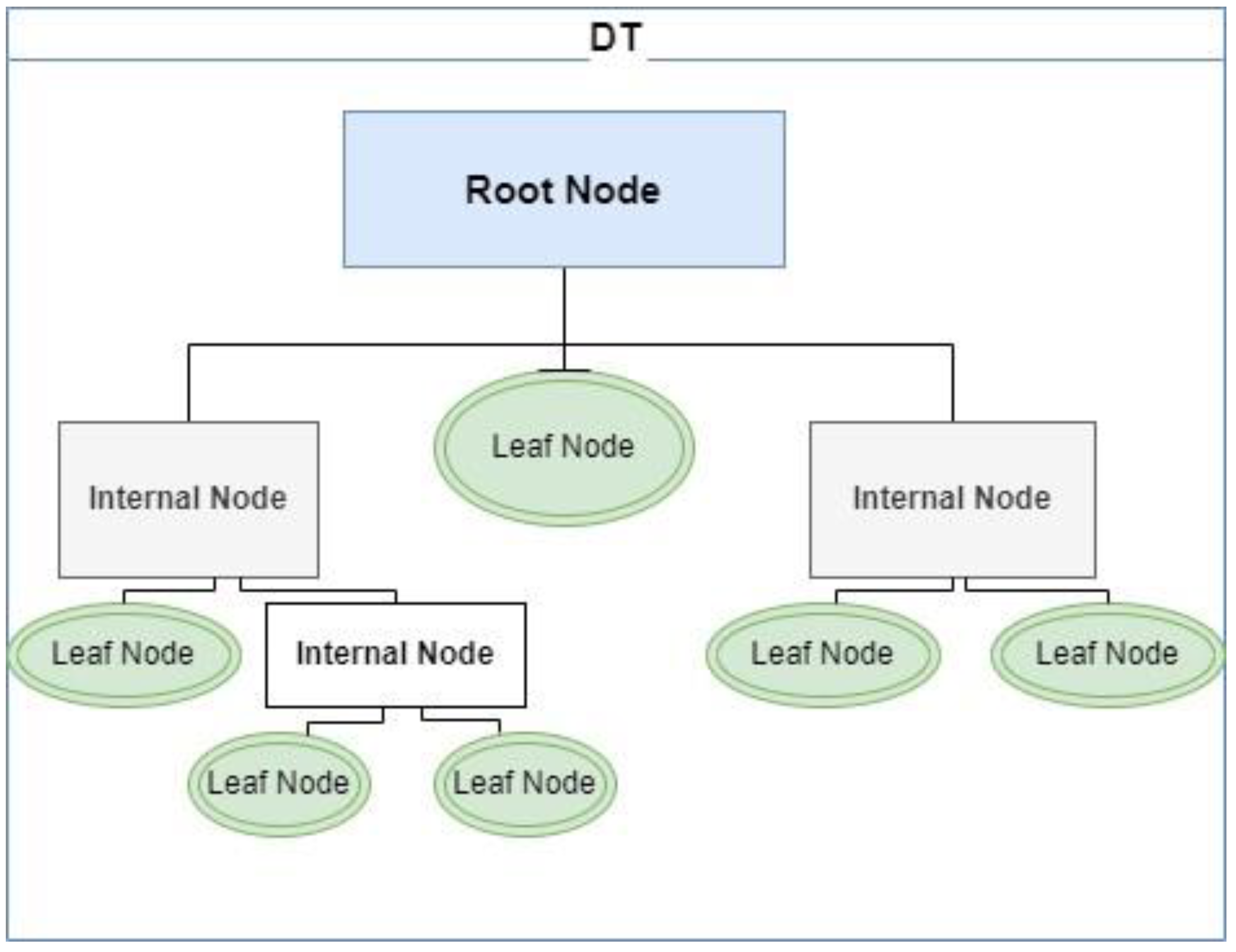
In the hierarchical order of the DT, the main root is located at the top node, as shown in Figure 2. Between the root and the leaves are internal nodes. The main purpose of constructing a DT is to find an attribute that needs to be retested at one node and then map it to another node [54]. In the DT model used in this study, the trees were not pruned.

2.2.2. Random Forest

RF is a supervised learning algorithm and ensemble model consisting of decision trees. The forest is made up of multiple decision trees created using the bagging technique. In essence, random forest constructs numerous decision trees and merges their results to achieve better accuracy and stability in prediction [21]. It can manage nonlinear, high-dimensional variables and is capable of handling outliers and noise. Furthermore, RF offers crucial benefits, such as relative variable importance and partial dependency plots, making the interpretation of RF results effortless. RF is widely employed for classification and regression tasks, as illustrated by Breiman (1996) [55] and Wan et al. (2023) [56].
Machine learning models have demonstrated superior predictive ability compared to traditional approaches. However, the black-box nature of many ML algorithms remains a challenge, as their inner workings are not easily interpreted [57,58,59]. The performance of machine learning algorithms can be enhanced by tuning their hyperparameters. Random forest (RF) has several advantages, including high resistance to overfitting and noise in the data. Additionally, this algorithm can handle large feature sets and perform well on datasets with missing data. The learning algorithm can generate a specific number of trees by using the “n_estimators” parameter or by passing a seed to randomize the trees with the “random_state” parameter [55]. In this study, we limited the number of trees generated to 200.

2.2.3. K-Nearest Neighbors

K-NN algorithm is a type of supervised learning method. It proves to be an uncomplicated algorithm for classifying or predicting regression values. Furthermore, the algorithm is considered “lazy” because it does not make generalizations on training data points, keeping them during the testing phase [60]. The classification or regression value of an example is computed by analyzing the similarities between each data sample in the dataset.
The k-NN algorithm consists of two steps. Firstly, it identifies the k training samples that are closest to the unknown sample. Secondly, it selects the class in which k samples occur most frequently. k-NN classification is typically used when all attributes are continuous [61]. The k-NN algorithm utilizes memorization instead of learning the training data. When prediction is required, it searches for the closest neighbors to the entire dataset. In addition to the Euclidean distance function, the Manhattan, Hamming, and Minkowski functions can also be used [62]. A k value of 1 means that the predictions of the new patterns to be predicted are made using the closest single training sample. The value of k can vary depending on the size of the dataset. In this study, we used Manhattan distance as the distance parameter because of the presence of both continuous and categorical variables.

2.2.4. Support Vector Machines

SVM is a commonly utilized machine learning algorithm that was developed in the 1990s. It is a supervised algorithm [63] and is used in both classification and regression problems. SVM separates data in either a linear or nonlinear manner, making it a versatile tool [64]. SVM can yield favorable outcomes despite the presence of noisy data. The benefits of the SVM algorithm consist of high accuracy, strong generalization properties, a limited number of hyperparameters, and proficiency in processing multidimensional data. Nevertheless, processing large datasets can be time-intensive, and selecting an appropriate kernel function is crucial.
The SVM algorithm is used to solve classification problems. It classifies data using a hyperplane that best separates the dataset into two classes. The chosen hyperplane provides the best margin to separate the classes of data. Margin refers to the distance between the data classes and the hyperplane. SVM can be used to classify both linearly separable and nonlinearly separable data. SVM works by selecting a hyperplane that maximizes the margin between two classes in linearly separable data. In cases where the data cannot be linearly separated, SVM transforms the data into a high-dimensional feature space using the kernel trick [63,64]. SVM uses various parameters, including the complexity parameter that controls the flexibility of the line used to separate classes. A value of 0 enforces a strict margin, while the default value is 1. Another crucial parameter is the kernel type. The linear kernel is the simplest and separates data with a straight line or hyperplane. A polynomial kernel separates data into classes using a curve or curved line. The strength of the separation decreases as the polynomial exponent value increases. The radial basis function (RBF) kernel, which is the most popular and powerful kernel, uses closed polygons and complex shapes to separate classes. This study employs linear, polynomial, and radial basis function kernels with default parameters. The input vectors are mapped nonlinearly on a high-dimensional plane, and a linear decision surface is formed on this plane to ensure the generalizability of the learning machine.

2.2.5. GridSearchCV

Grid Search Cross Validation (GridSearchCV) is a method for optimizing hyperparameters in machine learning algorithms. It seeks to improve model performance by selecting the most suitable dataset features. GridSearchCV tests all potential combinations within a specified set of hyperparameters to determine the ones that deliver the best results [65,66].
Previous studies have primarily employed grid search to explore the parameter space. However, this approach can be computationally intensive, particularly when dealing with high-dimensional parameter spaces. As an alternative, Bayesian optimization is often less computationally demanding. In our study, we employed grid search to explore values in the high-dimensional parameter space, which is a powerful technique for selecting high-quality parameters of machine learning problems [21]. Despite the high dimensionality of the parameter space, we used grid search to explore the parameter space. This is because the GridSearchCV method is well-suited to our problem and scales well. Testing each unique hyperparameter combination in the search space took a reasonable amount of time to determine the best-performing combination.

3. Experiment

3.1. Study Area

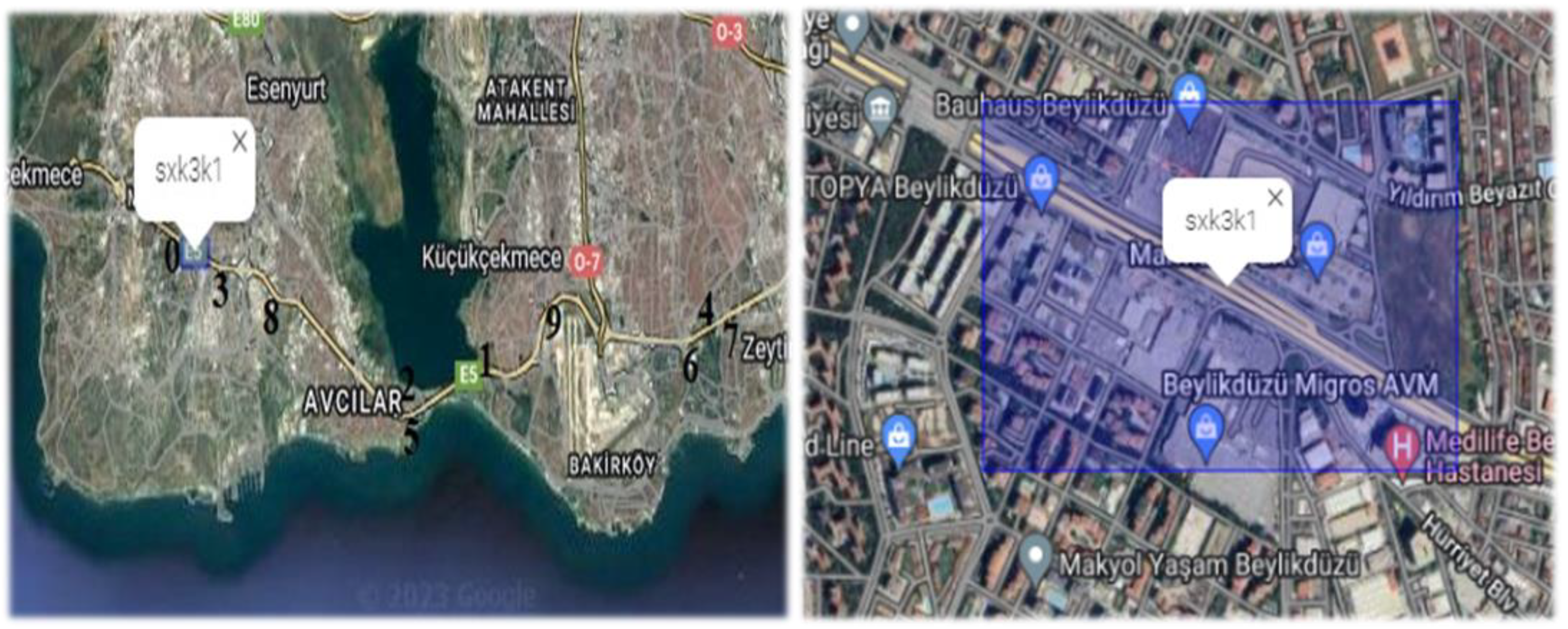
Istanbul was selected as the location for predicting traffic incidents in our study due to the high frequency of accidents and traffic incidents in the metropolis, which can lead to significant traffic flow disruptions in an already heavily congested city. During the data collection phase, the coordinates of the accidents and incidents were recorded and assigned a 6th geohash code with the use of ArcGIS software. The study’s data entail records of traffic accidents such as vehicle collisions and barrier collisions, as well as incidents like vehicle malfunctions, road fires, and traffic-related altercations. The total number of traffic incidents in Istanbul was recorded within 682 geohash areas, with each geohash area measuring 1.22 × 0.61 km2. Basic statistics of traffic incidents occurring in all defined areas were extracted, and the frequencies of traffic incidents occurring in these areas were obtained. When the 16-month data used in the study were examined, it was seen that there were no frequent accidents in most of the 682 defined areas. Narrowing the study area is predicted to improve the accuracy of predicting accident locations in Istanbul, which is a densely populated metropolis comprising 682 distinct zones that exhibit varying characteristics and accident rates. Due to the high occurrence of traffic incidents such as accidents, vehicle breakdowns, and road deformations in Beylikduzu-Bakirkoy, with a total of 5114 incidents, and the similarity of road conditions across all defined locations, this region was chosen as the study area. The substantial number of accidents/incidents in the region presents an opportunity to estimate the risky region with a large dataset. Furthermore, the adjacent geohash areas within the same region allow for the problem to be evaluated within a homogeneous region in Istanbul. Figure 3 shows the 10 geohash areas selected for the analysis and also the region specifically covered by geohash code 0.
The number of traffic incidents for 10 geohash areas with similar characteristics selected in this region is shown in Table 3. According to the table, 378 incidents occurred in the area with the fewest traffic incidents, and 654 accidents/incidents occurred in the area with the most traffic incidents.
The study defined a time interval in four periods, as outlined in Table 4, during which traffic incidents occurred at the identified locations. The highest frequency of incidents took place between 8 a.m. and 8 p.m., attributed to increased commuting for work, school, hospital, and other reasons. Few accidents occurred during sleeping hours, given the reduced traffic on roads.

3.2. Data Acquisition

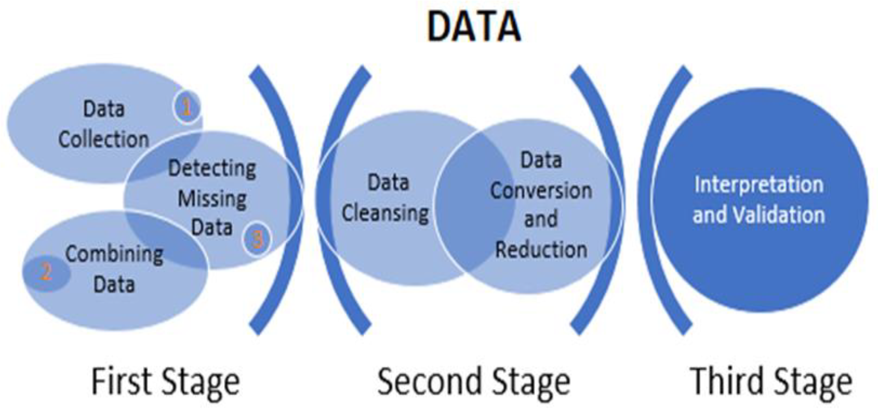
To achieve success in machine learning models, thorough and precise data collection is crucial for accurate predictions in the targeted area. We obtained data on traffic incidents from various national institutions and open data portals, including the Istanbul Metropolitan Municipality, the Turkish Statistical Institute, and the Turkish State Meteorological Service, as well as ArcGIS, IMM Open Data Portal, Development Library, OpenStreetMap, and Google Maps. The study analyzed various datasets, which were combined after pre-processing to gather necessary variables for predicting locations of traffic incidents. Data pre-processing steps are given in Figure 4.
During merging, ArcGIS and geohash codes were used to separate coordinate information for the variables and group them based on location. The research dataset comprises data on 74 variables in ten categories. A concise description of these categories is provided below, while complete information and descriptions of all variables are presented in Appendix A:
  • Time-dependent variables include year, month, day, special day, and incident time.
  • Location-dependent variables consist of latitude, longitude, geohash (output), and region, among others.
  • Vehicle variables encompass cars, trucks, and motorcycles, among others.
  • Variables related to traffic index include minimum, maximum, and average traffic index as well as traffic density.
  • Speed-related variables consist of minimum, maximum, and average speed and the number of vehicles per day.
  • Road structure and condition variables include road type, number of lanes, and divided road information.
  • Meteorological variables include temperature, humidity, wind speed and direction, road temperature, and rainfall amount.
  • Social and demographic variables include the number of schools, hospitals, residences, cafes/restaurants, and workplaces.
  • District-related variables consist of population, number of neighborhoods, agricultural area, surface area, etc.

3.3. Hyperparameter Tuning

Hyperparameters are configurable settings that need to be established by the user before training a machine learning model. It is essential to carefully fine-tune hyperparameters as it is a critical stage in training any machine learning model. Thus, accurate determination of hyperparameters can have a significant impact on resulting accuracy levels. Tools like GridSearchCV optimize critical hyperparameters, such as the learning rate and the batch size of the model, in cases where some hyperparameters have been specified. Precisely tuning these hyperparameters is crucial to maximize accuracy levels, increase computational efficiency, and avoid common issues like overfitting [67,68,69].
The GridSearchCV algorithm can perform cross-validation on models while simultaneously searching for their optimal parameters. The performance of each model is impacted to varying degrees by different parameters. Table 5 provides details on the parameters for the four machine learning algorithms employed.

3.4. Performance Matrix

Various measures are used to evaluate the effectiveness of classification-algorithm-generated models to determine the optimal model. One of these measures is the creation of a confusion matrix. In the fields of machine learning and statistics, a confusion matrix is a valuable instrument for assessing the classification models’ efficiency [48]. The 2 × 2 grid presented in this matrix displays four unique combinations resulting from the comparison of actual and predicted class values, as depicted in Table 6.
Each cell in the matrix depicts a unique classification outcome, facilitating the assessment of the model’s accuracy and efficacy. The investigation employed performance indicators such as accuracy, precision, recall, and F-measure scores.
Accuracy, the primary metric used for evaluating models, signifies the number of correct predictions out of all predictions. An algorithm for classification is deemed accurate when it correctly identifies a certain percentage of the sample. As shown formulaically below, accuracy is determined by dividing the sum of true positives (TP) and true negatives (TN) by the total number of samples (TP, TN, false positives (FP), and false negatives (FN).
A c c u r a c y = T P + T N T P + T N + F P + F N
The precision measures the proportion of accurately classified samples in a given category, specifically the percentage that are true positives. The precision is calculated using the following formula:
P r e c i s i o n = T P T P + F P
Recall indicates the accuracy of classifying a specific category. It shows how precisely a class was categorized. Recall is computed as
R e c a l l = T P T P + F N
The F1-Score is a statistical measure that combines precision and recall. It is commonly defined as the harmonic mean of the two values. F1-score is calculated with the following formula:
F 1 S c o r e = 2   P r e c i s i o n R e c a l l P r e c i s i o n + R e c a l l
Matthews correlation coefficient (MCC) is a measure used to evaluate the performance of classification models. MCC is computed as
M C C = T P T N F P F N T P + F P T P + F N T N + F P T N + F N  

3.5. Setup for the Experiment

Four distinct machine learning algorithms were implemented in our investigation utilizing the Scikit-learn library in Python in order to forecast the location of traffic incidents in Istanbul. The utilized machine learning models, including DT, RF, k-NN, and SVM, underwent optimization with the hyperparameter optimization technique resulting in a significant increase in model efficiency. With the aid of ArcGIS, we identified the geohash areas where most traffic accidents, vehicle breakdowns, and other traffic incidents took place in Istanbul, and we carefully examined 10 geohash areas accordingly. The study utilized a total of 5114 traffic incident data, depending on 74 input variables, to generate a classification problem for geohash fields. During the experiment, we tested different ratios for test and training data and found that the best outcome was obtained when the test data were 20% and the training data were 80%, using four distinct machine learning algorithms. Consequently, we randomly selected 4091 traffic incidents from diverse time periods over 16 months as training data, while the remaining 1023 traffic incidents were employed as test data.
The experiments were performed in the Anaconda3 2021.05 environment using Python version 3.8.8 (64-bit) on a computing system equipped with an Asus Intel(R) Core (TM) i5-8265U CPU running at 2.10 GHz (with a turbo boost frequency of 2.59 GHz), an Intel (R) graphics processing unit, and 16 GB of RAM. Windows 10 was the operating system used for these experiments.

4. Results

Performance metrics such as accuracy, precision, recall, and F1-score were computed to evaluate the effectiveness of the DT, k-NN, RF, and SVM algorithms employed. The results of the study are presented in Table 7, which highlights the performance of the four distinct machine learning models.
Table 7 displays that although random forest (RF) offers the highest accuracy rate of 90,8% for predicting traffic incident locations, other machine learning algorithms also deliver notable performance. The sequence of algorithm success in classification was RF, SVM, DT, and k-NN. The close distribution of traffic events within the 10 geohash clusters prevented over-learning of the training dataset, resulting in similar macro and micro precision, recall, and F1-scores. In RF, Precision_macro minimizes error costs to 8.5% and attains a success rate of 91.5%.
When evaluating the other performance metrics and situations where the correct and incorrect identifications were reversed, a 9% error was observed. Guessing the truth accurately and identifying errors in the wrong place showed significant performance in differentiating the clusters. This finding will be a valuable point of reference for further studies in the literature.
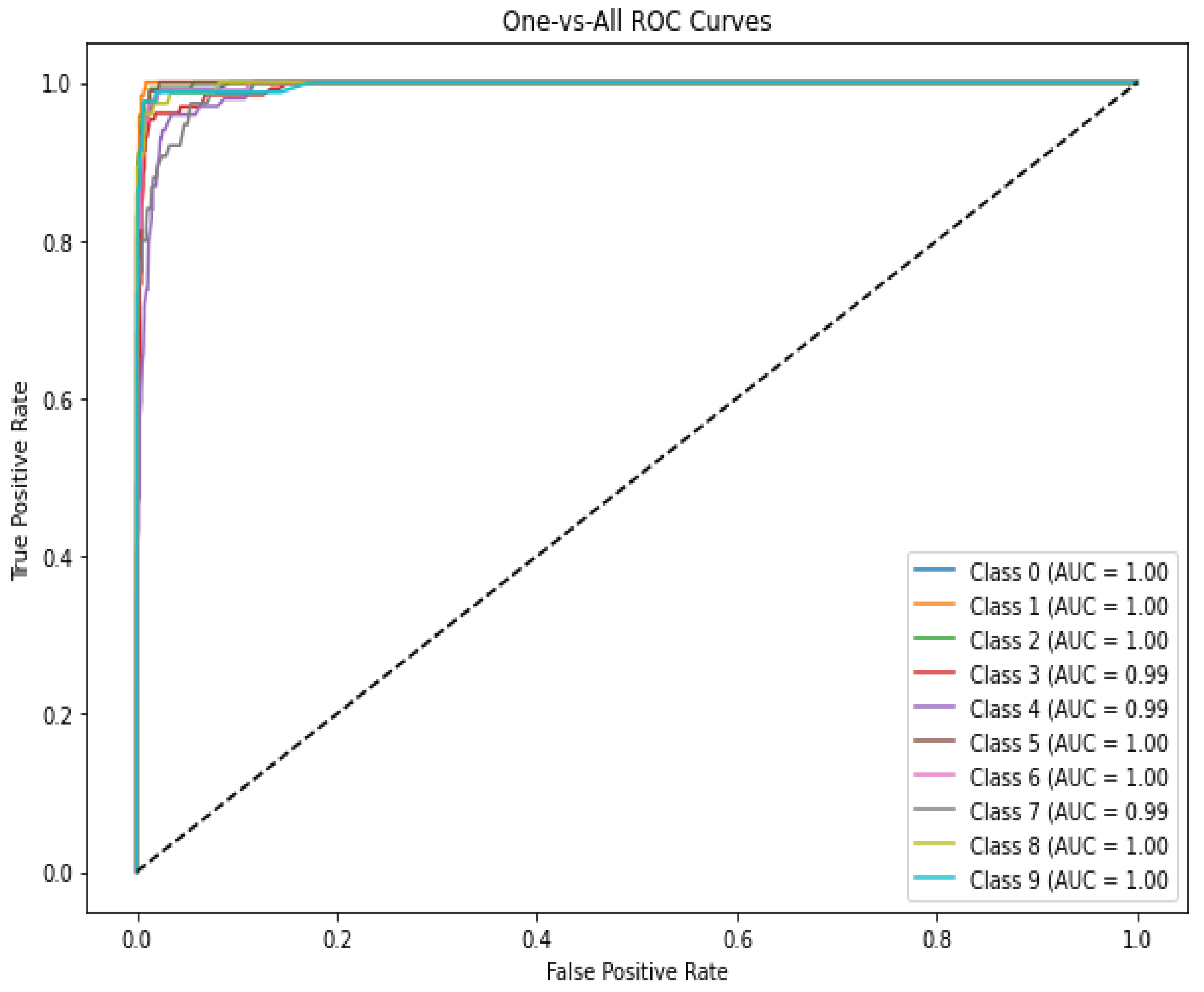
MCC is an evaluation metric that takes into account the imbalance between classes, especially in unbalanced classification problems. MCC value takes a value between −1 and 1. In our study, the MCC value of the RF model was calculated as 0.93. The closer the value of MCC is to 1, the better the performance of the RF model is. Additionally, the Roc_Auc graph of the RF model is given in Appendix B.
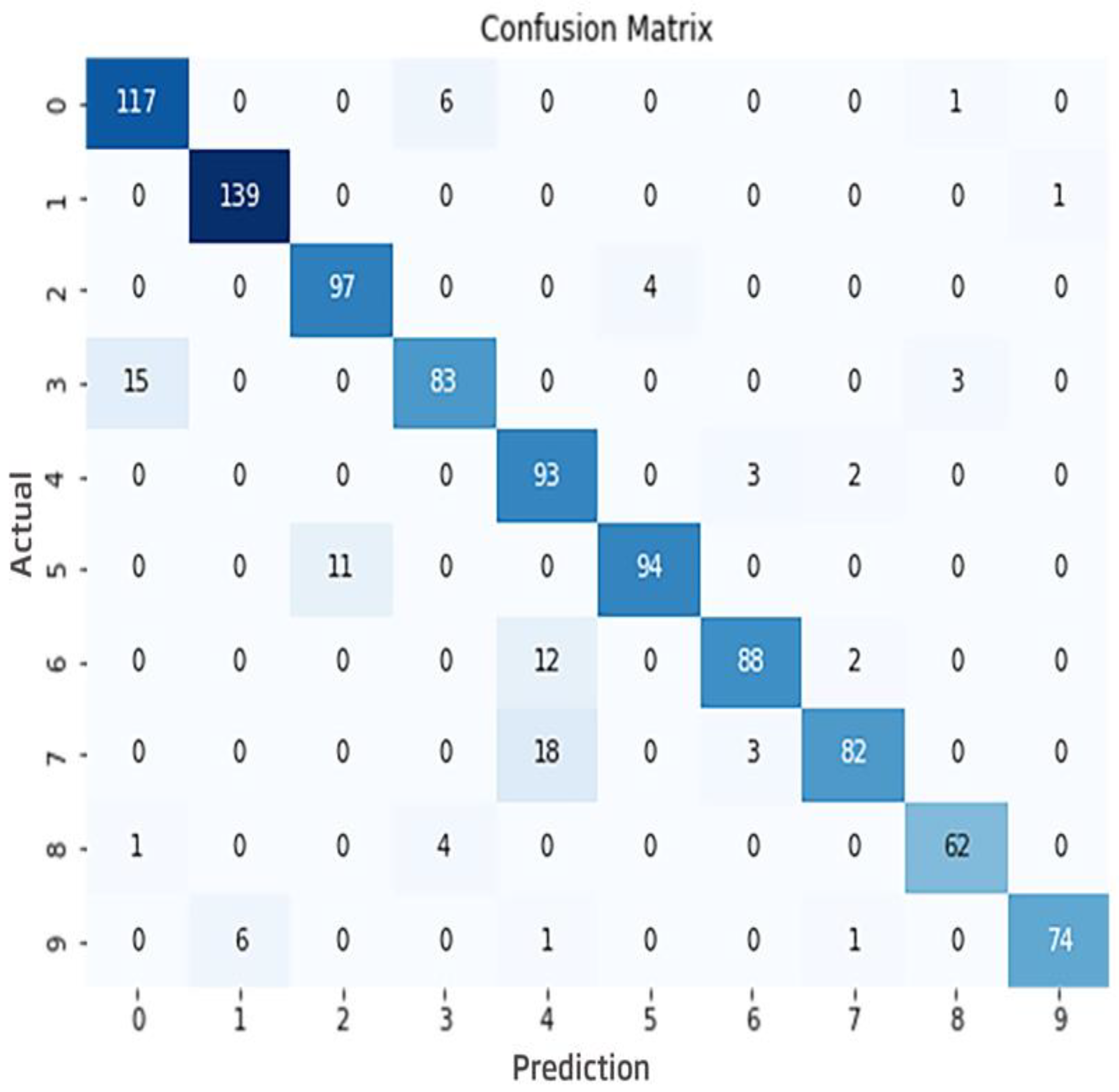
Figure 5 displays the confusion matrix for the RF model, which produced the most favorable outcomes. Confusion matrices for the other three models are included in Appendix B.
The confusion matrix depicted in Figure 5 illustrates how clusters representing geohash areas are distributed according to the test results obtained from 1023 traffic data. The confusion matrix shows a high number of correctly predicted instances, indicating the model’s success in predicting traffic event locations. Each class has a relatively high number of correctly predicted instances, demonstrating successful identification. From the test dataset, it is evident that the first geohash region had the highest number of traffic incidents reported with 140 occurrences, while the eighth geohash region had the lowest count of traffic events with only 67 incidents. A prediction accuracy of 99% was achieved as 139 out of 140 traffic incident locations in the first cluster were predicted correctly. The cluster indices with accuracy rates exceeding 90% for predicting traffic incident locations are 1, 2, 4, 0, 8, and 9, from the largest to the smallest. On the other hand, clusters 7, 3, 6, and 5 have accuracy rates lower than 90% when arranged numerically from the least to the most accurate. It was observed that cluster 7 had an accuracy rate of only 80%, and cluster 4 presented significant difficulty in predicting the traffic incident. It is understood that these two clusters are neighboring locations bordering each other, which explains the mixing situation. The close proximity of the regions allows for a relaxed approach, resulting in an 80% accuracy rate. Upon examining cluster 3, 15 traffic incidents that should have occurred were found to be in cluster 0 due to the two geohash fields being very close to each other. Twelve traffic incident locations that should be in cluster 6 were found to be in cluster 4, which are not close to each other. Although the model was unable to fully distinguish them, it achieved an acceptable 86% accuracy rate, representing a significant outcome for the ten cluster assignments. In clusters 1, 2, and 5, incorrect predictions were confused with only one cluster. Cluster 9 was confused with the highest number of different clusters, with a total of three. This indicates that the model’s incorrect predictions were primarily due to confusion between regions that are close to each other. Conversely, predictions for regions that are relatively distant from each other were more accurate.
A total of 1023 traffic accident-incidents that occurred in four different time intervals, (8:00 a.m.–1:59 p.m., 2:00 p.m.–7:59 p.m., 8:00 p.m.–1:59 a.m., and 2:00 a.m.–7:59 a.m.) in ten different geohash areas over a period of 16 months were used as test data. Table 8 displays the actual and predicted results of the traffic incidents that occurred in these various time periods and locations.
Upon examining the table, it becomes clear that 29 out of 33 traffic incidents that took place between 8:00 a.m. and 1:59 p.m. in geohash field number 5 were accurately forecasted. Thirty-three traffic events occurred at various times during the test period in the geohash area 1. During the first time period between 08:00 and 13:59 in the fifth region, our model successfully predicted 29 of the events. According to the table, the prediction success rate for 10 traffic incidents in time zone 1 is 92.48%. Out of the 27 incorrect predictions made in time zones, the largest amount occurred in the geohash field no. 7, with a total of 8 incorrect predictions. Notably, these incorrect predictions occurred within two adjacent geohash areas that produced the most errors.
In time zone 2, ten locations where traffic incidents are likely to occur were predicted with an accuracy rate of 90.16%. Among them, 44 incorrect predictions were made for the traffic incident location, and the majority of the errors occurred in geohash field number 3, with 11 incorrect predictions. These predictions erroneously estimated the incident location in geohash field 0. Here, as in nearby areas previously observed, the proximity of these locations contributes to the occurrence of these errors.
Ten traffic incidents were accurately predicted at a rate of 91.57% in time zone 3. However, the accuracy rate dropped to 82.35% in time zone 4, which corresponds to the early morning hours with relatively little traffic. This suggests that the prediction success decreases due to the scarcity of traffic events during this period. Compared to other time intervals, the success rate of learning from traffic events is relatively low during the fourth hour.

5. Conclusions

This study demonstrates the effectiveness of a geohash-based prediction model in estimating the locations of traffic incidents. The algorithms produced accurate and dependable estimations of incident locations. The suggested algorithm for predicting traffic incidents achieved a substantial accuracy rate of 90.81%. The use of geohash areas, combined with the consideration of all variables affecting traffic events, greatly influenced the success of the model. Analysis of geohash areas revealed that machine learning algorithms achieved remarkable success in predicting traffic incident locations through the use of geohash-area-based geographical data.
RF, SVM, and k-NN are generally more complex and flexible models. RF works as an ensemble learning method. In this case, it involves creating a strong learner by using multiple weak learners (DT). Ensemble learning increases overall performance by combining different learning strategies. A single tree model such as DT may overfit the training data, leading to overfitting. RF is more resistant to overfitting because it trains trees with random samples and features. For this reason, it gave the best results. SVM and k-NN are generally more flexible and powerful in terms of feature selection. This allows the model to make better use of important features in the dataset.
The prediction model enables dynamic geohash-based predictions. It captures real-time data, allowing for dynamic prediction of traffic incident scenes. Taking into account different time zones is also significant for the model’s ability to quickly adapt to traffic situations. The study’s findings indicate that precise analysis of geographic data, coupled with efficient utilization of geohash-based machine learning algorithms, can substantially aid in forming strategies to mitigate adverse consequences of traffic incidents. These results extend fresh insights to traffic managers and emergency responders on more effective management of traffic incidents to enhance the safety of drivers.
The model’s ability to successfully forecast can be used for automatic alerts and emergency management when integrated into traffic management systems. For example, when high probabilities of traffic incidents are detected in a given area, the system can automatically send alerts and mobilize emergency teams. Predicted traffic incident locations give traffic managers the chance to respond to incidents in advance. In this case, it can help traffic management systems utilize their resources more effectively and better plan emergency responses.
If real-time data from various variables, which may impact traffic accidents and incidents involving cities, traffic conditions, vehicles, and people, are incorporated into the model along with the flow of real-time data collected from various institutions’ databases, traffic events that are likely to occur within specific time frames can be predicted with high accuracy rates, apart from the 74 variables already included in the model. This can significantly improve traffic management and safety by optimizing traffic flow within cities and reducing adverse effects caused by traffic incidents. The prediction model will assist traffic supervisors and emergency response teams in precisely intervening at crucial sites and efficiently managing personnel during traffic incidents.

5.1. Limitations

This study has some limitations. Firstly, it focuses only on a specific region of Istanbul, namely Beylikduzu-Bakirkoy, which may limit the generalizability of the results. Secondly, it uses data from a specific time period covering a period of 16 months. Including a longer time frame may provide a more comprehensive analysis. Thirdly, the use of geohash fields is associated with a certain level of geographical precision.
When considering smaller geographical areas, forecasting success may be more challenging, but it can lead to more precise area estimation. On the other hand, if larger geographical areas are taken into account using geohash codes, prediction success may increase, but location accuracy may decrease. Additionally, the study’s model selection and evaluation metrics are based on a specific preference. These results could have been different if a specific algorithm or metric had been chosen.

5.2. Future Research

This study focuses on a specific geographical region. Future research could assess the effectiveness of a similar model in different cities, regions, or countries. Examining the impact of various geographical conditions, cultural factors, and traffic regulations can provide a more comprehensive understanding of the model’s general applicability. Additionally, comparing changes in traffic incident locations over time with ongoing traffic incidents in that area can be useful. Periodic factors should be analyzed in addition to feature selection to comprehensively address the factors affecting traffic incidents.
Our study introduced an innovative approach based on geohash, utilizing ArcGIS and machine learning algorithms. Future research could develop a more comprehensive approach by integrating different variables and various data sources not included in the current study into the model. In addition to the research conducted, gathering and consolidating real-time data from the various analyzed regions could potentially lead to significant advancements in future studies. This approach provides the advantage of predicting traffic incidents instantaneously, thus allowing for a swift response by emergency response teams.

Author Contributions

Conceptualization, M.U.; methodology, M.U.; software, M.U.; validation, Y.S.T. and M.U.; formal analysis, M.U.; investigation, M.U.; resources, E.K.; data curation, M.U. and Y.S.T.; writing—original draft preparation, M.U.; writing—review and editing, Y.S.T.; visualization, M.U. and Y.S.T.; supervision, M.U. and Y.S.T.; project administration, Y.S.T. and E.K. All authors have read and agreed to the published version of the manuscript.

Funding

This research received no external funding.

Institutional Review Board Statement

Not applicable.

Informed Consent Statement

Not applicable.

Data Availability Statement

Contact the corresponding author if interested in using data. The data are not publicly available due to privacy.

Conflicts of Interest

The authors declare no conflicts of interest.

Appendix A

VariablesData TypeExplanation
YearNumericYear of traffic incident
MonthCategoricalMonth in which the traffic incident occurred (1–12)
DayCategoricalDay of the month in which the traffic incident occurred (1–31)
Special dayCategoricalRepresentation of public holidays, religious holidays, and important days
Incident DayCategoricalDay of the week when the traffic incident occurred (1–7)
Time periodCategoricalTime range of the day when the traffic incident occurred (1 8–14, 2 14–20, 3 20–2, 4 2–8)
DistrictCategoricalDistricts where traffic incidents occur such as Avcilar, Bakirkoy, Bahcelievler, etc.
District populationNumericPopulation information of the district where the traffic incident occurred
Number of NeighborhoodsNumericNumber of neighborhoods in the district where the traffic incident occurred
Area measurementNumericArea of the district where the traffic incident took place
Minimum speedNumericMinimum speed for the relevant geohash area on the given day and time
Maximum speedNumericMaximum speed for the relevant geohash area on the given day and time
Average speedNumericAverage speed for the relevant geohash area on the given day and time
Number of unique vehiclesNumericNumber of different vehicles within the relevant geohash area on the given day and time
Minimum traffic indexNumericField containing minimum traffic index information on the relevant day and time
Maximum traffic indexNumericField containing maximum traffic index information on the relevant day and time
Average traffic indexNumericField containing average traffic index information on the relevant day and time
Number of vehicles per dayNumericTotal number of vehicles passing within the given day and the relevant geohash area
Daily average speedNumericAverage speed of vehicles on the given day and within the relevant geohash area
Traffic percentageNumericPercentage of overall traffic measured at five-minute intervals on a given day
TemperatureNumericAir temperature of the relevant district on the given day and time
Road temperatureNumericRoad temperature information of the relevant district on the given day and time
HumidityNumericAir humidity rate of the relevant district on the given day and time
Rainfall AmountNumericRainfall amount of the relevant district on the given day and time
Wind speedNumericWind speed of the relevant district on the given day and time
Wind directionNumericDirection of the wind speed of the relevant district on the given day and time
Ground informationCategoricalGround information of the relevant geohash area (dry/wet, etc.) on the given day and time
Road type-1CategoricalRoad type of the relevant geohash area (access road, side road, intersection, bridge, etc.)
Road type-2CategoricalRoad type in the relevant geohash area (main artery, highways, etc.)
Number of lanesCategoricalNumber of stripes of the relevant geohash area
Divided roadCategoricalDivided road information of the relevant geohash area
SpeedNumericCurrent speed limit
WidthNumericWidth of the road in the relevant geohash area
One WayCategoricalOne-way information of the road in the relevant geohash area
CarNumericNumber of cars registered in the relevant month and district
MinibusNumericNumber of minibuses registered in the relevant month and district
BusNumericNumber of buses registered in the relevant month and district
VanNumericNumber of vans registered in the relevant month and district
TruckNumericNumber of trucks registered in the relevant month and district
MotorcycleNumericNumber of motorcycles registered in the relevant month and district
Special purpose vehicleNumericNumber of special purpose vehicles registered in the relevant month and district
Total number of vehiclesNumericTotal number of vehicles in the relevant month
Bachelor’s degree rateNumericRate of people with a bachelor’s degree by year in the given district
Illiteracy rateNumericYear-based illiteracy rate of the given district
Student rateNumericYear-based student rate for the given district
Average household sizeNumericYear-based average household size for the given district
Number of housesNumericMonthly number of houses in the given district
Number of private workplacesNumericMonthly number of private workplaces in the given district
Agricultural fieldNumericYear-based agricultural area of the given district
Number of hospitalsNumericYear-based number of hospitals in the given district
Number of schoolsNumericYear-based number of schools in the given district
UniversityNumericYear-based number of universities in the given district
University facilityNumericNumber of university facilities in the given district
PoliceNumericYear-based number of police officers in the given district
Fire stationNumericYear-based fire department area of the given district
personSOSNumericYear-based number of emergency healthcare workers in the given district
Metrobus stationNumericYear-based number of metrobus stations in the given district
Metro stationNumericYear-based number of metro stations in the given district
PortNumericYear-based number of ports for the given district
Number of parking lotsNumericYear-based number of parking lots in the given district
Number of banksNumericYear-based number of banks in the given district
Number of ATMsNumericYear-based number of ATMs in the given district
Number of shopping mallsNumericYear-based number of shopping malls in the given district
Number of marketsNumericYear-based number of markets in the given district
Number of mini marketsNumericYear-based number of minimarkets in the given district
Number of super marketsNumericYear-based number of supermarkets in the given district
Number of hotelsNumericYear-based number of hotels in the given district
Number of storesNumericYear-based number of stores in the given district
Industrial areaNumericYear-based industrial area amount for the given district
Number of bars/clubsNumericYear-based number of bars/clubs in the given district
Number of cafesNumericYear-based number of cafes in the given district
Number of museum galleriesNumericYear-based number of museums and galleries in the given district
Sports facilityNumericYear-based number of sports facilities in the given district
Number of theatersNumericYear-based number of theater halls in the given district

Appendix B

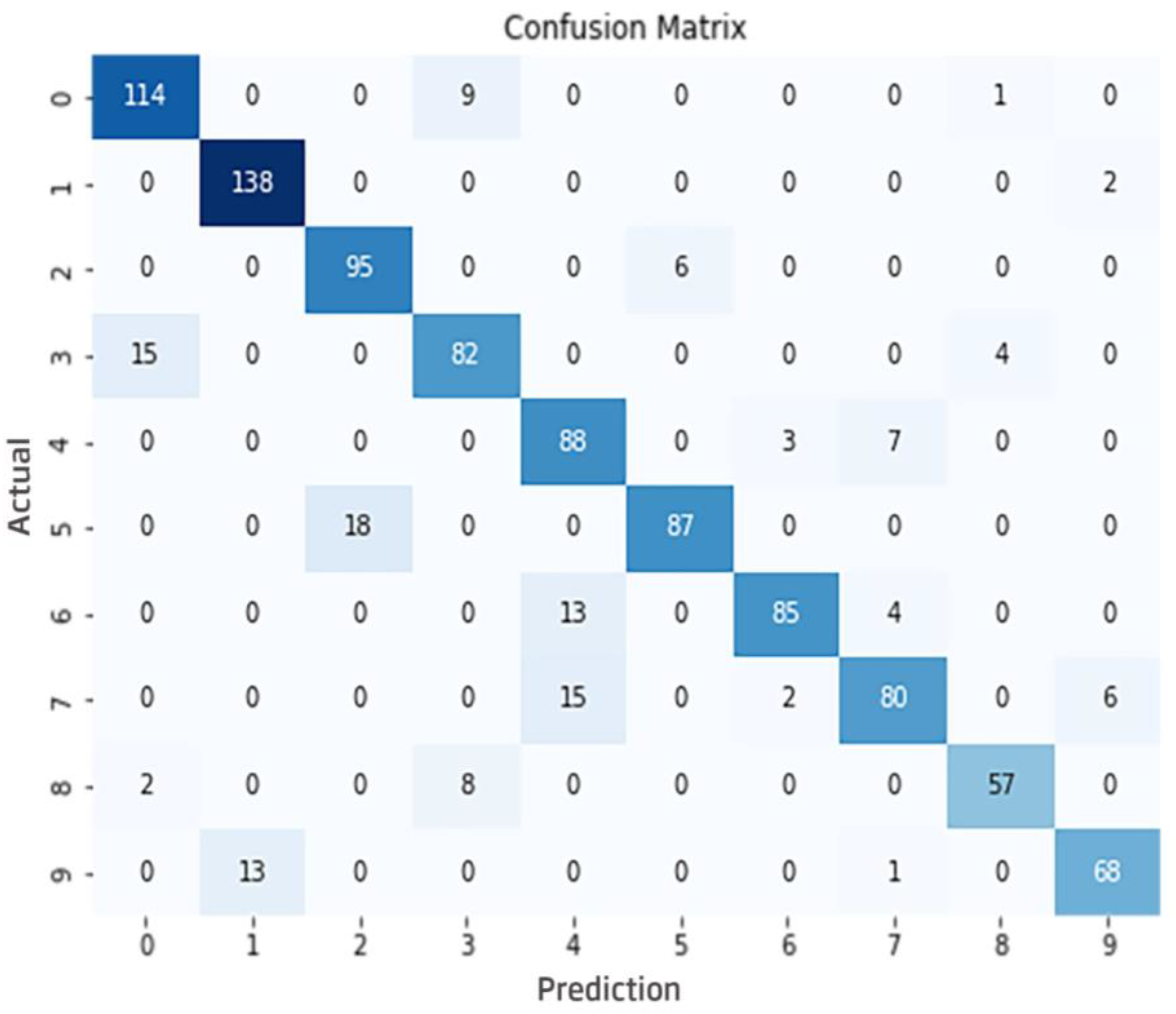
Figure A1. DT model confusion matrix.
Applsci 14 00725 g0a1
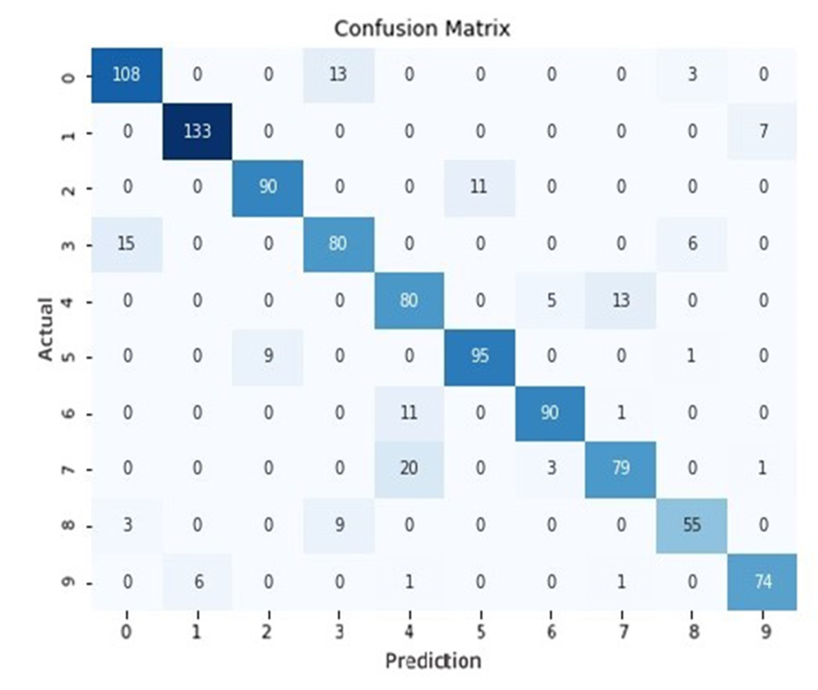
Figure A2. k-NN model confusion matrix.
Applsci 14 00725 g0a2
Figure A3. SVM model confusion matrix.
Applsci 14 00725 g0a3
Figure A4. Roc_Auc graph of RF model.
Applsci 14 00725 g0a4

References

  1. Helman, D.L. Traffic incident management. Public Roads 2004, 68, 14–21. [Google Scholar]
  2. Farrag, S.G.; Outay, F.; Yasar, A.U.H.; Janssens, D.; Kochan, B.; Jabeur, N. Toward the improvement of traffic incident management systems using Car2X technologies. Pers. Ubiquitous Comput. 2021, 25, 163–176. [Google Scholar] [CrossRef]
  3. Farrag, S.G.; Sahli, N.; El-Hansali, Y.; Shakshuki, E.M.; Yasar, A.; Malik, H. STIMF: A smart traffic incident management framework. J. Ambient Intell. Humaniz. Comput. 2021, 12, 85–101. [Google Scholar] [CrossRef]
  4. Wang, C.; Quddus, M.A.; Ison, S.G. The effect of traffic and road characteristics on road safety: A review and future research direction. Saf. Sci. 2013, 57, 264–275. [Google Scholar] [CrossRef]
  5. Touahmia, M. Identification of risk factors influencing road traffic accidents. Eng. Technol. Appl. Sci. Res. 2018, 8, 2417–2421. [Google Scholar] [CrossRef]
  6. Zou, Y.; Zhang, Y.; Cheng, K. Exploring the impact of climate and extreme weather on fatal traffic accidents. Sustainability 2021, 13, 390. [Google Scholar] [CrossRef]
  7. Ulu, M.; Türkan, Y.S.; Mengüç, K. Trafik kazalarını etkileyen faktörlerin ağırlıklarının BWM ve SWARA yöntemleri ile belirlenmesi. Akıllı Ulaşım Sist. Ve Uygulamaları Derg. 2022, 5, 227–238. [Google Scholar] [CrossRef]
  8. Xiang, W. An efficient location privacy preserving model based on Geohash. In Proceedings of the 2019 6th International Conference on Behavioral, Economic and Socio-Cultural Computing (BESC), Beijing, China, 28–30 October 2019; pp. 1–5. [Google Scholar]
  9. Zhang, Z.; Sun, X.; Chen, S.; Liang, Y. LPPS-AGC: Location privacy protection strategy based on alt-geohash coding in location-based services. Wirel. Commun. Mob. Comput. 2022, 2022, 3984099. [Google Scholar] [CrossRef]
  10. Basheer Ahmed, M.I.; Zaghdoud, R.; Ahmed, M.S.; Sendi, R.; Alsharif, S.; Saad, B.A.A.; Alsabt, R.; Rahman, A.; Krishnasamy, G. A real-time computer vision based approach to detection and classification of traffic incidents. Big Data Cogn. Comput. 2023, 7, 22. [Google Scholar] [CrossRef]
  11. Grigorev, A.; Mihaita, A.S.; Lee, S.; Chen, F. Incident duration prediction using a bi-level machine learning framework with outlier removal and intra–extra joint optimisation. Transp. Res. Part C Emerg. Technol. 2022, 141, 103721. [Google Scholar] [CrossRef]
  12. Li, L.; Sheng, X.; Du, B.; Wang, Y.; Ran, B. A deep fusion model based on restricted Boltzmann machines for traffic accident duration prediction. Eng. Appl. Artif. Intell. 2020, 93, 103686. [Google Scholar] [CrossRef]
  13. Zhao, Y.; Deng, W. Prediction in traffic accident duration based on heterogeneous ensemble learning. Appl. Artif. Intell. 2022, 36, 2018643. [Google Scholar] [CrossRef]
  14. Gutierrez-Osorio, C.; González, F.A.; Pedraza, C.A. Deep Learning Ensemble Model for the Prediction of Traffic Accidents Using Social Media Data. Computers 2022, 11, 126. [Google Scholar] [CrossRef]
  15. Lin, D.J.; Chen, M.Y.; Chiang, H.S.; Sharma, P.K. Intelligent traffic accident prediction model for Internet of Vehicles with deep learning approach. IEEE Trans. Intell. Transp. Syst. 2021, 23, 2340–2349. [Google Scholar] [CrossRef]
  16. Chuanxia, S.; Han, Z.; Peixuan, Y. Machine learning and IoTs for forecasting prediction of smart road traffic flow. Soft Comput. 2023, 27, 323–335. [Google Scholar] [CrossRef]
  17. Bai, M.; Lin, Y.; Ma, M.; Wang, P.; Duan, L. PrePCT: Traffic congestion prediction in smart cities with relative position congestion tensor. Neurocomputing 2021, 444, 147–157. [Google Scholar] [CrossRef]
  18. Liu, Y.; Wu, C.; Wen, J.; Xiao, X.; Chen, Z. A grey convolutional neural network model for traffic flow prediction under traffic accidents. Neurocomputing 2022, 500, 761–775. [Google Scholar] [CrossRef]
  19. An, J.; Fu, L.; Hu, M.; Chen, W.; Zhan, J. A Traffic congestion prediction in smart cities with relative position network method to traffic flow prediction with uncertain traffic accident information. IEEE Access 2019, 7, 20708–20722. [Google Scholar] [CrossRef]
  20. Quek, C.; Pasquier, M.; Lim, B. A novel self-organizing fuzzy rule-based system for modelling traffic flow behaviour. Expert Syst. Appl. 2009, 36, 12167–12178. [Google Scholar] [CrossRef]
  21. Yan, M.; Shen, Y. Traffic accident severity prediction based on random forest. Sustainability 2022, 14, 1729. [Google Scholar] [CrossRef]
  22. Vaiyapuri, T.; Gupta, M. Traffic accident severity prediction and cognitive analysis using deep learning. Soft Comput. 2021, 1–13. [Google Scholar] [CrossRef]
  23. Yang, Z.; Zhang, W.; Feng, J. Predicting multiple types of traffic accidents using deep learning techniques. Cluster-task deep learning framework. Saf. Sci. 2022, 146, 105522. [Google Scholar] [CrossRef]
  24. Santos, D.; Saias, J.; Quaresma, P.; Nogueira, V.B. Machine learning approaches to traffic accident analysis and hotspot prediction. Computers 2021, 10, 157. [Google Scholar] [CrossRef]
  25. Zhang, Z.; Yang, W.; Wushour, S. Traffic accident prediction based on LSTM-GBRT model. J. Control Sci. Eng. 2020, 2020, 4206919. [Google Scholar] [CrossRef]
  26. Godumula, D.T.; Ravi Shankar, K.V.R. Safety evaluation of horizontal curves on two lane rural highways using machine learning algorithms: A priority-based study for sight distance improvements. Traffic Inj. Prev. 2023, 24, 331–337. [Google Scholar] [CrossRef]
  27. Ferreira-Vanegas, C.M.; Vélez, J.I.; García-Llinás, G.A. Analytical methods and determinants of frequency and severity of road accidents: A 20-year systematic literature review. J. Adv. Transp. 2022, 145, 7239464. [Google Scholar] [CrossRef]
  28. Lin, Y.; Li, R. Real-time traffic accidents post-impact prediction: Based on crowdsourcing data. Accid. Anal. Prev. 2020, 145, 105696. [Google Scholar] [CrossRef]
  29. Zhang, C.; Li, Y.; Li, T. A road traffic accidents prediction model for traffic service robot. Libr. Hi Tech 2002, 40, 1031–1048. [Google Scholar] [CrossRef]
  30. Gan, J.; Li, L.; Zhang, D.; Yi, Z.; Xiang, Q. An alternative method for traffic accident severity prediction: Using deep forests algorithm. J. Adv. Transp. 2020, 2020, 1257627. [Google Scholar] [CrossRef]
  31. Park, R.C.; Hong, E.J. Urban traffic accident risk prediction for knowledge-based mobile multimedia service. Pers. Ubiquitous Comput. 2022, 26, 417–427. [Google Scholar] [CrossRef]
  32. Azhar, A.; Rubab, S.; Khan, M.M.; Bangash, Y.A.; Alshehri, M.D.; Illahi, F.; Bashir, A.K. Detection Predicting multiple types of deep learning techniques. Clust. Comput. 2023, 26, 477–493. [Google Scholar] [CrossRef]
  33. Rahman, M.T.; Jamal, A.; Al-Ahmadi, H.M. Examining hotspots of traffic collisions and their spatial relationships with land use: A GIS-based geographically weighted regression approach for Dammam, Saudi Arabia. ISPRS Int. J. Geo-Inf. 2020, 9, 540. [Google Scholar] [CrossRef]
  34. Qu, X.; Meng, Q. A note on hotspot identification for urban expressways. Saf. Sci. 2014, 66, 87–91. [Google Scholar] [CrossRef]
  35. Anderson, T.K. Kernel density estimation and K-means clustering to profile road accident hotspots. Accid. Anal. Prev. 2009, 41, 359–364. [Google Scholar] [CrossRef]
  36. Macedo, M.R.; Maia, M.L.; Rabbani, E.R.K.; Neto, O.C.L.; Andrade, M. Traffic accident prediction model for rural highways in Pernambuco. Case Stud. Transp. Policy 2022, 10, 278–286. [Google Scholar] [CrossRef]
  37. Moons, E.; Brijs, T.; Wets, G. Identifying hazardous road locations: Hot spots versus hot zones. In Transactions on Computational Science VI; Springer: Berlin/Heidelberg, Germany, 2009; pp. 288–300. [Google Scholar]
  38. Shariff, S.R.; Maad, H.A.; Halim, N.N.A.; Derasit, Z. Determining hotspots of road accidents using spatial analysis. Indones. J. Electr. Eng. Comput. Sci. 2018, 9, 146–151. [Google Scholar]
  39. Al-Omari, A.; Shatnawi, N.; Khedaywi, T.; Miqdady, T. Prediction of traffic accidents hot spots using fuzzy logic and GIS. Appl. Geomat. 2020, 12, 149–161. [Google Scholar] [CrossRef]
  40. Al-Aamri, A.K.; Hornby, G.; Zhang, L.C.; Al-Maniri, A.A.; Padmadas, S.S. Mapping road traffic crash hotspots using GIS-based methods: A case study of Muscat Governorate in the Sultanate of Oman. Spat. Stat. 2021, 42, 100458. [Google Scholar] [CrossRef]
  41. Manap, N.; Borhan, M.N.; Yazid, M.R.M.; Hambali, M.K.A.; Rohan, A. Identification of hotspot segments with a risk of heavy-vehicle accidents based on spatial analysis at controlled-access highway. Sustainability 2021, 13, 1487. [Google Scholar] [CrossRef]
  42. Erdogan, S.; Yilmaz, I.; Baybura, T.; Gullu, M. Geographical information systems aided traffic accident analysis system case study: City of Afyonkarahisar. Accid. Anal. Prev. 2008, 40, 174–181. [Google Scholar] [CrossRef]
  43. Liang, L.Y.; Ma’soem, D.M.; Hua, L.T. Traffic accident application using geographic information system. J. East. Asia Soc. Transp. Stud. 2005, 6, 3574–3589. [Google Scholar]
  44. Mali, S. Traffic police operation based on sensors and data analytics. Transp. Res. Procedia 2020, 47, 187–194. [Google Scholar] [CrossRef]
  45. Feng, Y.; Zhu, W. Formulating an Innovative Spatial-Autocorrelation-based Method for Identifying Road Accident Hot Zones. IOP Conf. Ser. Earth Environ. Sci. 2020, 446, 052068. [Google Scholar] [CrossRef]
  46. Alkhadour, W.; Zraqou, J.; Al-Helali, A.; Al-Ghananeem, S. Traffic accidents detection using geographic information systems (GIS). Int. J. Adv. Comput. Sci. Appl. 2021, 12, 484–494. [Google Scholar] [CrossRef]
  47. Xie, K.; Ozbay, K.; Yang, D.; Xu, C.; Yang, H. Modeling bicycle crash costs using big data: A grid-cell-based Tobit model with random parameters. J. Transp. Geogr. 2021, 91, 102953. [Google Scholar] [CrossRef]
  48. Ulu, M. Trafik Olay Yönetiminde Yapay Zeka Tabanlı Bir Optimizasyon Modeli ve Uygulaması. Doctoral Dissertation, Istanbul University–Cerrahpasa, Istanbul, Türkiye, 2023. [Google Scholar]
  49. Menguc, K.; Aydin, N.; Yilmaz, A. A Data Driven Approach to Forecasting Traffic Speed Classes Using Extreme Gradient Boosting Algorithm and Graph Theory. Phys. A Stat. Mech. Its Appl. 2023, 620, 128738. [Google Scholar] [CrossRef]
  50. Huang, K.; Li, G.; Wang, J. Rapid retrieval strategy for massive remote sensing metadata based on GeoHash coding. Remote Sens. Lett. 2018, 9, 1070–1078. [Google Scholar] [CrossRef]
  51. Suwardi, I.S.; Dharma, D.; Satya, D.P.; Lestari, D.P. Geohash index based spatial data model for corporate. In Proceedings of the 2015 International Conference on Electrical Engineering and Informatics (ICEEI), Denpasar, Indonesia, 10–11 August 2015; IEEE: Piscataway, NJ, USA, 2015; pp. 478–483. [Google Scholar]
  52. GeoHash. Available online: https://learn.microsoft.com/tr-tr/azure/data-explorer/kusto/query/geo-point-to-geohash-function (accessed on 10 June 2023).
  53. Quinlan, J.R. Induction of decision trees. Mach. Learn. 1986, 1, 81–106. [Google Scholar] [CrossRef]
  54. Vanfretti, L.; Arava, V.N. Decision tree-based classification of multiple operating conditions for power system voltage stability assessment. Int. J. Electr. Power Energy Syst. 2020, 123, 106251. [Google Scholar] [CrossRef]
  55. Breiman, L. Bagging predictors. Mach. Learn. 1996, 24, 123–140. [Google Scholar] [CrossRef]
  56. Wan, M.; Wu, Q.; Yan, L.; Guo, J.; Li, W.; Lin, W.; Lu, S. Taxi drivers’ traffic violations detection using random forest algorithm: A case study in China. Traffic Inj. Prev. 2023, 24, 362–370. [Google Scholar] [CrossRef]
  57. Dwivedi, Y.K.; Hughes, L.; Ismagilova, E.; Aarts, G.; Coombs, C.; Crick, T.; Duan, Y.; Dwivedi, R.; Edwards, J.; Eirug, A.; et al. Artificial Intelligence (AI): Multidisciplinary perspectives on emerging challenges, opportunities, and agenda for research, practice and policy. Int. J. Inf. Manag. 2021, 57, 101994. [Google Scholar] [CrossRef]
  58. Rudin, C.; Radin, J. Why are we using black box models in AI when we don’t need to? A lesson from an explainable AI competition. Harv. Data Sci. Rev. 2019, 1, 1–9. [Google Scholar]
  59. Raja, M.N.A.; Abdoun, T.; El-Sekelly, W. Smart prediction of liquefaction-induced lateral spreading. J. Rock Mech. Geotech. Eng. 2023. [Google Scholar] [CrossRef]
  60. Song, Y.; Liang, J.; Lu, J.; Zhao, X. An efficient instance selection algorithm for k nearest neighbor regression. Neurocomputing 2017, 251, 26–34. [Google Scholar] [CrossRef]
  61. Peterson, L.E. K-nearest neighbor. Scholarpedia 2009, 4, 1883. [Google Scholar] [CrossRef]
  62. Abu Alfeilat, H.A.; Hassanat, A.B.; Lasassmeh, O.; Tarawneh, A.S.; Alhasanat, M.B.; Eyal Salman, H.S.; Prasath, V.S. Effects of distance measure choice on k-nearest neighbor classifier performance: A review. Big Data 2019, 7, 221–248. [Google Scholar] [CrossRef]
  63. Jakkula, V. Tutorial on Support Vector Machine (Svm); School of EECS, Washington State University: Pullman, WA, USA, 2006; Volume 37, p. 3. [Google Scholar]
  64. Alpaydin, E. Machine Learning: The New AI; MIT Press: Cambridge, MA, USA, 2016. [Google Scholar]
  65. Géron, A. Hands-on Machine Learning with Scikit-Learn, Keras, and TensorFlow; O’Reilly Media, Inc.: Sebastopol, CA, USA, 2022. [Google Scholar]
  66. Liao, L.; Li, H.; Shang, W.; Ma, L. An empirical study of the impact of hyperparameter tuning and model optimization on the performance properties of deep neural networks. ACM Trans. Softw. Eng. Methodol. (TOSEM) 2022, 31, 1–40. [Google Scholar] [CrossRef]
  67. Liang, E.; Stamp, M. Predicting pedestrian crosswalk behavior using Convolutional Neural Networks. Traffic Inj. Prev. 2023, 24, 338–343. [Google Scholar] [CrossRef]
  68. Raschka, S. Python Machine Learning; Packt Publishing Ltd.: Birmingham, UK, 2015. [Google Scholar]
  69. Radhakrishnan, P. What are Hyperparameters? And How to tune the Hyperparameters in a Deep Neural Network? Data Sci. 2017, 18. [Google Scholar]
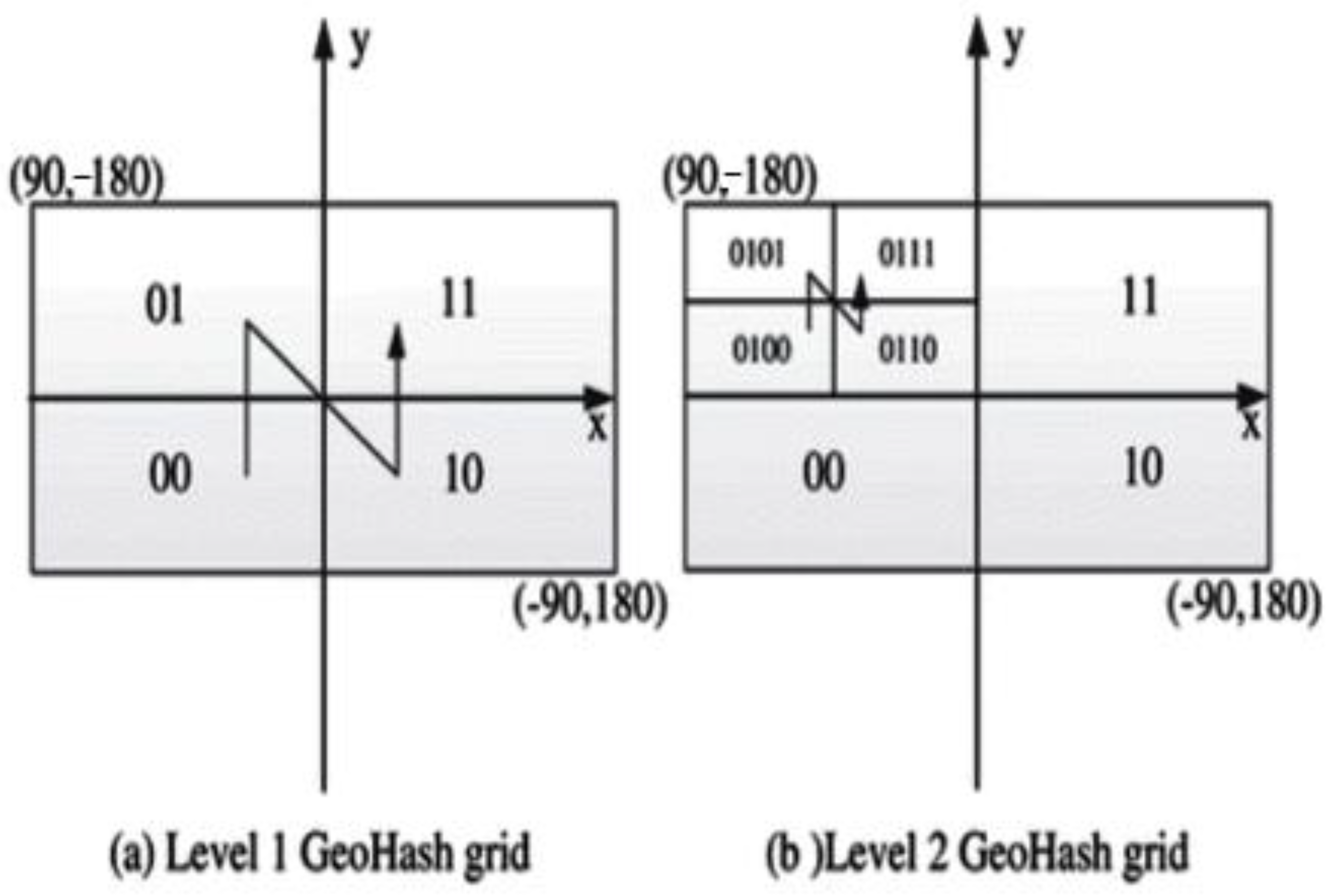
Figure 1. Geohash grid division diagram.
Applsci 14 00725 g001
Figure 2. Decision tree representation.
Applsci 14 00725 g002
Figure 3. Displayed geohash areas and 0th geohash area.
Applsci 14 00725 g003
Figure 4. Data pre-processing.
Applsci 14 00725 g004
Figure 5. RF model confusion matrix.
Applsci 14 00725 g005
Table 1. Geohash parameters.
NameDescription
LatitudeGeospatial coordinate is the latitude value in degrees. The valid value is a real number and is in the range [−90, +90].
LongitudeGeospatial coordinate is the longitude value in degrees. The valid value is a real number and is in the range [−180, +180].
AccuracyIt defines the requested level of accuracy. The supported values fall within the range of (1, 18). If a value is not specified, the default of 5 will be used.
Table 2. Geohash lengths/codes.
Geohash Length/CodeCell WidthCell Height
15000 km5000 km
21250 km625 km
3156.25 km156.25 km
439.06 km19.53 km
54.88 km4.88 km
61.22 km0.61 km
7152.59 m152.59 m
838.15 m19.07 m
94.77 m4.77 m
101.19 m0.59 m
11149.01 mm149.01 mm
1237.25 mm18.63 mm
Table 3. Frequency of traffic incidents.
IndexGeohashIncident Frequency
0sxk3k1654
1sxk3nt600
2sxk3ju561
3sxk3k2542
4sxk90z529
5sxk3n5510
6sxk90w463
7sxk91p472
8sxk3k8405
9sxk3pr378
Table 4. Traffic incident time interval.
Time IntervalsTraffic Incident Time IntervalIncident Frequency
108:00–13:591927
214:00–19:592148
320:00–01:59754
402:00–07:59285
Table 5. Parameters of the GridSearchCV algorithm.
DTk-NN
HyperparameterValueHyperparameterValue
max_depth3, 5, 7, Nonen_neighbors3, 5, 7, 9, 11
min_samples_split2, 5, 10weightsuniform, distance
min_samples_leaf1, 2, 4p1, 2, 3
RFSVM
HyperparameterValueHyperparameterValue
n_estimators50, 100, 200C0.1, 1, 10
max_depthNone, 5, 10kernellinear, poly, rbf
min_samples_split2, 5
min_samples_leaf1, 2, 4degree2, 3
Table 6. Confusion matrix [48].
Predicted PositivePredicted Negative
Actual PositiveTrue Positive (TP)False Negative (FN)
Actual NegativeFalse Positive (FP)True Negative (TN)
Table 7. Test results.
Performance MetricDTk-NNRFSVM
accuracy0.8740.7860.9080.875
balanced accuracy0.8670.7740.9050.872
precision micro0.8740.7860.9080.875
precision macro0.8780.7900.9150.876
recall micro0.8740.7860.9080.875
recall macro0.8670.7740.9050.872
f1 micro0.8740.7860.9080.875
f1 macro0.8700.7750.9070.873
Table 8. Actual and predicted traffic incidents.
Geohash
Area
Actual/
Predicted
1st
Time
Zone
2nd
Time
Zone
3rd
Time
Zone
4th
Time
Zone
Total
0Actual3868153124
Predicted3862143117
1Actual5052326140
Predicted5051326139
2Actual3639188101
Predicted333818897
3Actual27541010101
Predicted25437883
4Actual44409598
Predicted43379493
5Actual3346242105
Predicted294222194
6Actual4733175102
Predicted422814488
7Actual3347149103
Predicted254011682
8Actual21368267
Predicted19338262
9Actual303219182
Predicted282917074
Total
Incidents
359447166511023
Total
Predictions
33240315242929
Accuracy
Rate
92.4890.1691.5782.3590.81
Disclaimer/Publisher’s Note: The statements, opinions and data contained in all publications are solely those of the individual author(s) and contributor(s) and not of MDPI and/or the editor(s). MDPI and/or the editor(s) disclaim responsibility for any injury to people or property resulting from any ideas, methods, instructions or products referred to in the content.