Abstract
The incidence of bladder cancer is on the rise, and its molecular heterogeneity presents significant challenges for personalized cancer therapy. Transcriptome data can characterize the variability among patients. Traditional machine-learning methods often struggle with high-dimensional genomic data, falling into the ’curse of dimensionality’. To address this challenge, we have developed MVMSGAT, an innovative predictive model tailored for forecasting responses to neoadjuvant therapy in bladder cancer patients. MVMSGAT significantly enhances model performance by incorporating multi-perspective biological prior knowledge. It initially utilizes the Boruta algorithm to select key genes from transcriptome data, subsequently constructing a comprehensive graph of gene co-expression and protein–protein interactions. MVMSGAT further employs a graph convolutional neural network to integrate this information within a multiview knowledge graph, amalgamating biological knowledge maps from various scales using an attention mechanism. For validation, MVMSGAT was tested using a five-fold cross-validation approach on two specific GEO datasets, GSE169455 and GSE69795, involving a total of 210 bladder cancer samples. MVMSGAT demonstrated superior performance, with the following metrics (mean ± standard deviation): AUC-ROC of , accuracy of , F1 score of , and recall of . These results underscore the potential of MVMSGAT in advancing personalized treatment and precision medicine in bladder cancer.
1. Introduction
Bladder cancer, a prevalent malignancy in the urinary system, has an increasing annual incidence rate [1]. This cancer is classified as either non-muscle-invasive (NMIBC) or muscle-invasive (MIBC) based on the extent of bladder wall invasion. The main treatment for MIBC is radical cystectomy, often combined with neoadjuvant platinum-based chemotherapy [2]. However, due to bladder cancer’s molecular heterogeneity, responses to this therapy vary greatly among individuals [3]. Accurate prediction of treatment effectiveness prior to therapy commencement is crucial for personalized treatment strategies, improving cure rates, and minimizing the impact of ineffective therapies. However, reliable biomarkers for predicting MIBC patients’ responses to neoadjuvant therapy are still unidentified.
Genomic research is vital in advancing personalized cancer diagnosis and treatment [4]. Analyzing patients’ transcriptome data provides insights into the current state of cancer and its individual variability. Machine-Learning (ML) integration in biomedical research is creating new paths for cancer diagnostics and treatment [5,6]. ML models have predicted hepatocellular carcinoma recurrence with 74.19% accuracy using whole-genome data [7]. Other research has employed supervised ML methods for high-precision prediction of non-small cell lung cancer responses to immunotherapy [8]. Moreover, ML analysis of data from 762 breast cancer patients has led to the early detection of breast cancer and the identification of key biomarkers [9]. However, traditional pattern recognition methods face challenges in high-dimensional, low-sample datasets, known as the ’curse of dimensionality’.
Incorporating biological prior knowledge into these models can enhance their generalization ability and yield better results [10]. By integrating relevant biological information, models can more accurately navigate the complex genetic data landscape, leading to clinically relevant predictions [11]. Transforming biological knowledge into graph structures is advantageous, as graphs effectively represent complex biological system relationships and interactions [12]. This method allows for a more intuitive and thorough analysis of genetic data’s intricate connections. For instance, Graph Convolutional Networks (GCN) have been used to predict circular RNA-disease connections, outperforming traditional methods [13]. Another study combined GCN with biological knowledge graphs to identify genes linked to complex diseases [14]. These graph-based approaches have proven effective in enhancing model performance and stability.
In our study, we sought to predict the effectiveness of neoadjuvant therapy in bladder cancer patients using baseline transcriptome data, multiview knowledge graphs, and graph convolutional neural network techniques. Using the Boruta algorithm, we identified significant gene sets for constructing graph nodes related to treatment outcomes. Gene co-expression and protein–protein interaction networks were formed from these nodes, enriched with extensive biological knowledge. A multi-head graph attention convolutional neural network refined features, with pooling to extract multi-scale biomarkers. An attention mechanism combined features from different network layers for outcome prediction. This method improved our model’s accuracy and contributed to precision medicine. Our study’s key achievements include:
- 1.
- Creating a predictive model for bladder cancer patient responses to neoadjuvant therapy based on a multiview knowledge graph.
- 2.
- Using a multi-head graph attention mechanism to integrate gene co-expression and protein–protein interaction network features, capturing essential multi-scale features via pooling.
- 3.
- Demonstrating the model’s precision in predicting treatment responses, proving its competitive advantage over existing methods.
2. Review of Existing Work
In the context of personalized medicine, the unique biological information provided by a patient’s gene expression patterns is particularly crucial in determining which patients are likely to benefit from neoadjuvant therapy [4]. This section presents a review of studies focused on the selection of bladder cancer patients who benefit from neoadjuvant therapy.
Initial research concentrated on analyzing the expression levels of specific individuals’ genes, as these expressions are directly linked to the tumor’s sensitivity or responsiveness to treatment. For instance, a study of BRCA1 mRNA expression levels in 57 patients with advanced bladder cancer revealed that those with lower or moderate expression levels were more likely to benefit from neoadjuvant therapy (p = 0.01) [15]. This finding highlights the predictive value of BRCA1 expression levels in the efficacy of platinum-based neoadjuvant chemotherapy and could impact the formulation of personalized treatment strategies. The role of BRCA1 in DNA repair mechanisms may explain its association with treatment responsiveness. Additionally, in another study involving 50 patients receiving neoadjuvant therapy, whole-exome sequencing identified that patients with ERCC2 gene mutations were more likely to benefit from treatment (p < 0.01). ERCC2’s critical role in the DNA repair process may be the key link between its mutation and treatment efficacy [16]. An analysis of 178 cancer-related genes in 71 patients revealed that ERBB2 mutations were common among those who benefited from neoadjuvant therapy, although this result was not statistically significant, possibly due to limited sample size or high data variability [17]. Subsequent research shifted towards multi-gene analysis. For example, after conducting a differential gene expression analysis in 18 patients undergoing neoadjuvant therapy, researchers identified 14 genes with significant expression differences and developed a treatment effect prediction scoring system [18]. This system was tested in a validation cohort of 22 patients and successfully predicted the treatment outcomes in 19 patients, confirming the feasibility of using gene expression differences to construct a treatment effect prediction scoring system [19].
Although traditional statistical methods like the t-test and ANOVA have proven effective in multiple fields, they faced numerous challenges when handling large-scale biomarker data with numerous features, high dimensionality, and nonlinear relationships [20]. Genomic data, for instance, often do not conform to the assumption of a normal distribution and may contain outliers and biomarkers beyond detection limits, potentially skewing data distribution. To address these challenges, new ML techniques have been developed to handle large datasets, cope with complex data distributions, and address nonlinear issues.
This research based on models utilizing Support Vector Machine (SVM) algorithms has demonstrated the ability to accurately predict the response of individual cancer patients to various standard chemotherapy drugs based on tumor gene expression characteristics (such as RNA sequencing or microarray data), with an accuracy rate exceeding 80% [21]. This indicates the potential value of machine-learning algorithms in clinical applications, particularly in identifying effective second-line treatment options for patients who fail first-line standard treatments. Moreover, machine-learning methods have also been applied to early identification of patients with metastatic or recurrent colorectal cancer who are sensitive to FOLFOX therapy (a chemotherapy regimen combining 5-FU, leucovorin, and oxaliplatin) [22]. Researchers used microarray meta-analysis to identify differentially expressed genes (DEGs). These genes showed significant expression level differences between patients who responded to FOLFOX therapy and those who did not. These genes are closely associated with biological processes such as autophagy, ErbB signaling pathway, mitochondrial autophagy, endocytosis, FoxO signaling pathway, apoptosis, and resistance to antifolate drugs. Using these candidate genes, researchers applied various machine-learning algorithms and assessed the models’ performance through cross-validation methods. In other studies, machine-learning techniques have been used to predict responses to immunotherapy and neoadjuvant chemotherapy. For example, machine learning was utilized to explore the limitations of known drug mechanisms in predicting pathological complete response (pCR) and the impact of biological characteristics on response prediction in the first 10 treatment regimens of the I-SPY 2 trial [23]. Additionally, research has proposed a new classification of Hepatocellular Carcinoma (HCC) cancer stem cell-related using machine-learning algorithms based on RNA sequencing datasets to predict patients’ responses to immunotherapy [24].
Deep-learning technologies have shown significant potential in precision medicine, particularly in predicting the response of bladder cancer patients to neoadjuvant therapy. These algorithms, by analyzing patterns in complex biological and chemical data, can effectively predict how cancer cell lines and patients might respond to new drugs or drug combinations, therefore aiding in personalized treatment planning [25]. For instance, deep-learning models integrating gene expression, gene mutations, and compound chemical structures have significantly improved prediction accuracy in applications on GDSC and CCLE datasets by analyzing cancer-related gene and chemical information features [26]. The CDRscan model employs a dual-step convolutional architecture to process the gene mutation fingerprint of cell lines and the molecular fingerprint of drugs, and through “virtual docking”, it successfully identifies potential new cancer indications for existing drugs. Furthermore, models based on residual neural networks have been applied to NCI-60 drug pair screening data, focusing on drug combination activity, emphasizing the importance of drug descriptors in predicting cell line responses to drug pairings, and highlighting the potential of deep learning in predicting drug combination effects [27]. The DeepDR model, combining mutation encoders, expression encoders, and drug response predictors, has outperformed traditional methods in training on cancer cell lines and demonstrated potential in predicting tumor responses to drugs, providing insights into known and novel drug targets and drug resistance mechanisms [28]. These studies collectively illustrate the growing importance of deep learning in the field of cancer drug response prediction. By leveraging deep-learning technologies and integrating diverse genomic and chemical information data, these models are enhancing our understanding of drug responses and paving the way for more personalized and effective cancer treatments.
However, challenges remain in the current state of research. First, to date, graph convolutional neural networks have not been extensively applied in predicting the efficacy of neoadjuvant therapy for bladder cancer, representing an unexplored avenue with potential for significant impact. Second, the inherent complexity of genes poses a considerable challenge, with their intricate interactions and variations contributing to the difficulty in accurately predicting treatment outcomes. This complexity underscores the need for advanced computational models that can effectively decipher the nuances of genomic data in the context of bladder cancer therapy.
3. Materials and Methods
The detailed methodology of our approach is illustrated in Figure 1. We commence by selecting datasets from the Gene Expression Omnibus (GEO) Database that fulfill specific inclusion criteria, followed by preprocessing to negate batch effects, therefore ensuring data uniformity (Figure 1a). The Boruta algorithm is employed for feature selection, isolating a gene set highly correlated with treatment effectiveness for constructing the nodes of a multiview biological knowledge graph (Figure 1b). Subsequently, we analyze gene co-expression correlations and integrate protein–protein interaction networks to establish the edges of the graph. The MSMVGAT network updates node features, aggregates gene function clusters, and fuses multiview, multi-scale features for patient prediction (Figure 1c). Lastly, the model undergoes five-fold cross-validation to assess its generalization capabilities thoroughly (Figure 1d).
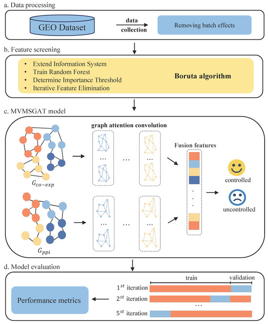
Figure 1.
Overview of the proposed method for bladder cancer treatment response prediction.
3.1. Boruta Algorithm for Feature Selection
Feature selection is a crucial step in building predictive models, improving both performance and accuracy [29]. Datasets usually contain many features, but not all are equally important for prediction. Some features can unintentionally add noise or redundancy, leading to model overfitting and reduced generalization ability. This issue is especially prominent in transcriptome sequencing data, which is known for its high dimensionality.
Among various feature selection methods, Boruta stands out [30]. Based on the Random Forest algorithm, Boruta excels in identifying and keeping all relevant features in a dataset while removing insignificant ones. Its effectiveness is not just theoretical; it has been proven in numerous medical datasets, as confirmed by several studies [31,32,33]. This evidence highlights Boruta’s role in boosting predictive accuracy and strengthening model robustness, especially in complex, high-dimensional data settings.
The Boruta algorithm has been adopted for feature selection. Rooted in the principles of the random forest methodology, Boruta assesses the import of original variables in contrast to a set of generated shadow features, facilitating the discernment of relevant variables from those deemed inconsequential. This algorithm exhibits robustness in handling diverse data typologies, including both categorical and numerical datasets, and is characterized by a reduced susceptibility to outlier influences. The utilization of Boruta contributes to the interpretability of the model, enabling a more profound comprehension of gene expression variables that are pivotal in the prediction of therapeutic efficacy. This approach is indicative of an in-depth appreciation of the complex and high-dimensional nature of genetic data, targeted towards the refinement of predictive accuracy in patient treatment outcomes. The steps of the Boruta algorithm are as follows:
- 1.
- Extend the information system by adding shadow attributes created by shuffling original ones.
- 2.
- Train a random forest classifier on the extended information system and gather the importance measure (e.g., Mean Decrease Accuracy) for all attributes.
- 3.
- Find the maximum Z score among shadow attributes (MZSA) and then assign a significance level to each attribute where the importance measure for a given attribute is higher than MZSA.
- 4.
- Remove all attributes that are confirmed to be less relevant than shadow attributes, and iterate the above steps until all attributes are confirmed or rejected.
The significance of original features is assessed using a Z test. The null hypothesis of this test is that a feature’s importance is not greater than that of the shadow features. The Z score, calculated as follows, helps determine this:
where M is the original attribute’s importance, and are the mean and standard deviation of the shadow attributes’ importance. Attributes with a Z score exceeding a predefined threshold, , are considered relevant.
3.2. Construction of Multiview Graphs
In our study, gene co-expression graphs are essential for elucidating the relational expression among various genes, thus contributing to an understanding of the molecular underpinnings of diseases. The construction of these graphs involved two principal components: gene expression correlations and protein–protein interaction (PPI) data.
3.2.1. Gene Co-Expression Graph
Gene co-expression networks play a key role in revealing complex relationships between gene expressions, offering valuable insights into disease mechanisms [34]. In our study, we began with a carefully selected set of genes, treating each gene as a node in a network graph. We used the Pearson correlation coefficient, which ranges from −1 to 1, to measure correlations between these genes [35]. A coefficient close to 1 implies a strong positive correlation, while a value close to −1 indicates a strong negative correlation. Values around 0 suggest no linear correlation. In constructing the network graph, we connected gene pairs only if the absolute value of their Pearson correlation coefficient exceeded a soft threshold of , indicating a substantial correlation, regardless of whether it is positive or negative. This threshold was chosen to ensure that only gene pairs with a significant level of correlation, either positive or negative, are included, therefore enhancing the biological relevance of the network. The Pearson correlation coefficient itself, when its absolute value is greater than 0.4, determines the weight of each edge, representing the significant strength of gene expression correlation.
3.2.2. Protein–Protein Interaction Graph
In addition to the gene co-expression graph, we integrated a PPI graph to explore the mechanisms of disease progression and evolution [36]. The PPI graph shows physical and functional connections between proteins, shedding light on their functionalities and interactions [37]. We gathered PPI data relevant to our selected genes from the STRING database [38]. Gene IDs were matched with their corresponding protein IDs. For genes linked to multiple proteins, we averaged the interaction weights to calculate an overall interaction weight between genes. By setting a soft threshold of , we have ensured that our analysis focuses on interactions with a substantial likelihood of biological significance. This threshold was chosen based on the STRING-score, reflecting a balance between including meaningful connections and excluding low-confidence ones [39]. This approach aims to provide a more accurate representation of the molecular interactions relevant to bladder cancer progression and response to neoadjuvant therapy.
3.3. Developing a Graph Attention Network across Multiple Perspectives and Scales
In the current study, we introduce a multi-perspective, multi-scale graph attention network, as depicted in Figure 2. This network is designed to integrate various biological datasets for predicting the response of bladder cancer patients to neoadjuvant therapy. The model inputs two distinct types of biological graphs: the gene co-expression graph , based on gene expression patterns, and the protein–protein interaction graph , which delineates the interplay among proteins. In these representations, and represent the nodes of the respective graphs, while and denote the corresponding edges.
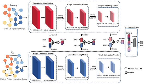
Figure 2.
Visualization of the MVMSGAT Network Architecture, highlighting the integration of two distinct biological graphs: the gene co-expression graph and the protein–protein interaction graph . For each graph, G is represented as where V denotes the node set, E denotes the edge set, and X denotes the node feature matrix. This representation captures the structure and attributes of the graph, with each layer beneath the network diagram indicating the number of nodes , the number of edges , and the feature-length at that layer. Such detail illustrates the evolving complexity and informational depth as the data progresses through the network.
Our approach involves capturing information from adjacent nodes through a Graph Embedding Module to update the information of the nodes themselves. Subsequently, we employ a TOP-k pooling operation to obtain a more compact graph representation. Following this, feature vectors for each graph dimension are extracted using a readout operation. The feature vectors from the gene co-expression graph and the protein–protein interaction graph, corresponding to the same dimension, are then fused through an attention mechanism. This step ensures the effective integration of information extracted from both graph types. Finally, the fused vectors across different dimensions are concatenated to form a comprehensive feature vector, which is then fed into a fully connected layer for the prediction of patient outcomes post-neoadjuvant therapy. These outcomes are classified into two categories: tumor controlled—Complete Response [CR], Partial Response [PR], and Stable Disease [SD]—and tumor uncontrolled—Progressive Disease [PD].
Through this methodology, our model leverages multi-scale graph representations and attention mechanisms to deeply understand the response of bladder cancer patients to neoadjuvant therapy, providing robust data support for personalized treatment strategies.
3.3.1. Node Feature Update Mechanism
In graph convolutional neural networks, node feature updates are achieved by aggregating features from neighboring nodes, enabling the network to discern local connectivity patterns [40]. This neighborhood-focused feature aggregation renders GCNs suitable for graph data analysis, facilitating direct engagement with graph structures and the acquisition of complex and advanced node feature representations, which offers deeper insights into various graph analysis tasks. In our research, we harnessed a multi-head graph convolutional neural network to independently extract features from two distinct graphs, and . Employing the graph attention network (GAT) with a multi-head attention mechanism, we updated the node features [41]. This framework allowed each node’s feature representation to be influenced not only by its inherent features but also by the weighted features of its adjacent nodes. This multi-head attention approach enabled each head to focus independently on varying information facets, allowing for a more comprehensive capture of the intricate inter-node interactions within the graph’s structure. This method is advantageous for generating distinctive feature representations, providing a potent means for decoding the complex information embedded within the graph. Attention coefficients for each node pair i and j were individually calculated for each head using the following formula:
where denotes the attention score between nodes i and j for the k-th head, computed as follows:
Here, signifies the linear transformation weight matrix for the k-th head, is the corresponding attention vector, and are the feature vectors for nodes i and j, respectively, and represents vector concatenation. Building upon the multi-head attention mechanism, we refined the node feature update process by layering multiple graph attention layers. Each node’s new feature was updated using the equation:
In this expression, denotes an activation function, and represents the weighted summation of the neighbors j of node i, incorporating neighbor information. The weighting , as derived from the described attention mechanism, signifies the degree of contribution from neighbor node j to node i, with representing the linear transformation weights for the head, and as the initial feature vector for node j.
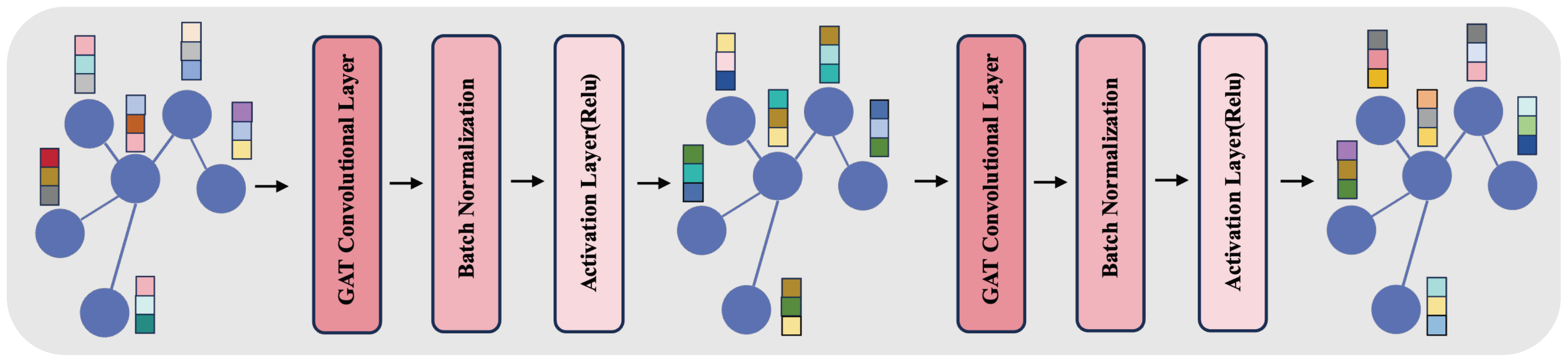
Additionally, our approach integrates a Graph Embedding Module, as depicted in Figure 3. This module employs a two-layered structure, each layer comprising a GAT convolutional layer followed by batch normalization and an activation layer (ReLU). In the GAT layers, we configure the number of channels to 128 and the number of heads to 8, enhancing the model’s ability to focus on different information facets within the graph. This architecture avoids the issues of over-smoothing and vanishing gradients, which are common in deeper networks. Batch normalization aids in stabilizing the training process, while ReLU introduces necessary non-linearity, enabling effective capture of complex patterns in the graph data.
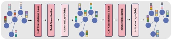
Figure 3.
The figure represents the Graph Embedding Module, showcasing a two-layer structure with GAT convolutional layers, each with 128 channels and 8 heads, batch normalization, and ReLU activation. This architecture aims to balance complexity and efficiency, addressing common challenges in deep networks while processing features from and graphs.
3.3.2. Aggregation of Functional Group Genes via TOP-K Pooling
Distinct functional gene groups possess unique biological significance, often representing specific biological processes and cellular functions. Our approach utilized the TOP-K pooling operation, set at a ratio of 0.8, to coalesce gene clusters exhibiting common biological functions [42,43]. This operation selects the top 80% of nodes based on their importance scores, computed via a learnable transformation followed by an activation function. Specifically, the importance score for a node i is determined using:
where is the weight matrix, is the attention vector, and is the feature vector of node i. Selection based on the score retains the top 80% of nodes deemed most crucial, discarding the remainder, therefore streamlining the graph’s complexity while capturing extensive biological information, providing robust feature representations for understanding disease mechanisms and predicting treatment responses.
3.3.3. Model Prediction via Multi-Scale Feature Fusion
In this study, feature fusion was conducted through an attention layer that integrated the gene co-expression graph with the protein–protein interaction graph . Global average pooling was employed to obtain the final layer of graph node features for each scale, represented as and , which were concatenated to yield , defined as . Attention weights for the combined feature were determined through a linear transformation and a sigmoid function, producing the fused feature . Subsequent to feature fusion, a multi-scale concatenation integrated feature information across different layers and scales, resulting in . The model then fed into a multi-layer perceptron for final predictions, with the treatment response prediction probability being the sigmoid output of the fully connected layer. Patient tumor control was designated as label 1, while tumor uncontrolled was labeled 0.
4. Experiment
4.1. Data Acquisition
Gene expression data and clinical information were obtained from two cohorts of bladder cancer patients with neoadjuvant treatment retrieved from the GEO database (https://www.ncbi.nlm.nih.gov/geo/(accessed on 24 September 2023)) with the accession numbers GSE169455 [44] and GSE69795 [45]. The criteria for study inclusion were as follows: (1) The cases were diagnosed with MIBC. (2) All patients received neoadjuvant treatment. (3) The cases had complete expression data. (4) For analysis of clinical characteristics, the patients had corresponding clinical and prognosis information. The dataset encompasses comprehensive clinical details and gene expression information, as delineated in the Supplementary Materials (see Tables S1 and S2). Furthermore, a concise summary of the principal attributes of the dataset, including sample size, platform, and data sources, is systematically tabulated in Table 1.

Table 1.
Characteristics of the GSE169455 and GSE69795 Datasets.
The integration of multiple datasets typically resulted in batch effects or non-biological variations. To tackle these effects, we utilized the empirical Bayes algorithm provided in the ComBat function of the SVA package during our data preprocessing phase [46]. This method was crucial for reducing batch-related discrepancies, therefore enhancing the overall quality and reliability of our data analysis.
4.2. Implementation Details
The programming language employed for the experiments was Python 3.9, provided by the Python Software Foundation, based in the Netherlands. The deep-learning tasks were facilitated by the PyTorch framework, which was developed by Facebook in the USA. Graphical computations were executed using an NVIDIA GeForce RTX 3090-TI GPU, supplied by NVIDIA, Santa Clara, CA, USA. The training process was configured with a batch size of eight and a learning rate set to . Loss computation was performed using the cross-entropy function, and the model was optimized with the AdamW algorithm, which incorporates weight decay.
5. Results
5.1. Construction of Multiview Graphs and Efficacy of Boruta Feature Selection
In our study, we effectively used the Boruta feature selection algorithm to identify genes crucial for bladder cancer treatment. We limited the algorithm’s random forest classifier to five layers to prevent overfitting and maintain simplicity. A key part of our analysis was setting the boruta_perc feature importance threshold at 80%. This threshold required a feature to be significant in at least 80% of 2400 iterations (boruta_max_iter = 2400) to be included.
We meticulously explored various boruta_perc thresholds to strike an optimal balance between retaining significant features and enhancing model performance. Ultimately, the 80% threshold was selected, ensuring the retention of pertinent features with no compromise on accuracy. Notably, the top 20 genes, ranked by their importance, are systematically presented in Table 2. Furthermore, a comprehensive list of all evaluated genes is available in Supplementary Materials Table S3 for detailed reference.
Table 2.
Top 20 genes by importance ranking: Gene abbreviations and their corresponding full names.
After selecting features, the gene co-expression network showed an average of 8.914 neighbors per node, a diameter of 8, and a clustering coefficient of 0.404, indicating moderate connectivity and a tendency for clustering. This is supported by a network density of 0.033, suggesting gene clusters often form closely connected groups. Detailed statistical information can be found in Table 3.
Table 3.
Topological statistics of the gene co-expression and protein–protein interaction networks.
Meanwhile, the PPI graph was larger, with 847 nodes and an average of 8.944 neighbors per node. Its diameter of 13 and radius of 7 indicate a more extensive network. The PPI network’s clustering coefficient of 0.25 suggested less clustering compared to the gene network. The PPI network, with more nodes and edges, appeared less clustered but more spread out. Its larger diameter and radius, along with a higher number of connected components, hint at a more fragmented structure. This fragmentation may reflect that a complex interaction landscape is important for understanding diseases.
Our analysis showed the value of examining bladder cancer treatment from two biological network perspectives. The PPI network, with 128 connected components, revealed complex protein interactions related to bladder cancer. In contrast, the gene co-expression network provided insights into gene interaction patterns. Integrating Boruta feature selection with multiview graph construction, we examined the biological complexities of bladder cancer. This method allowed us to gather comprehensive information from both networks, forming a robust biological knowledge base for future analysis and treatment outcome prediction.
5.2. Comparative Analysis of Predictive Models
In this study, we evaluated the performance of traditional machine-learning models, such as Support Vector Machines (SVM), Decision Trees (DT), Random Forests (RF), and Gradient Boosting Decision Trees (GBDT), against advanced graph-based models like Graph Attention Networks (GAT), Multi-Scale Graph Attention Networks (MSGAT), and Multiview Multi-Scale Graph Attention Networks (MVMSGAT). The traditional models were optimized using grid search to find the best combination of parameters, ensuring optimal model performance. Furthermore, to assess the robustness and consistency of these models, we employed a five-fold cross-validation method. This approach divides the dataset into five parts, using one as the test set and the others for training in rotation, thus minimizing fluctuations in model performance across different data splits.
We also explored advanced graph-based models such as GAT, MSGAT, and MVMSGAT. GAT introduces an attention mechanism to weight neighboring nodes’ features, enabling the model to focus on key information. MSGAT expands upon this by incorporating multi-scale processing, capturing both local node features and overall graph structure. MVMSGAT further extends this approach by combining data from multiple views, capturing richer and more comprehensive graph structure features across multiple scales.
In evaluating these models, we used metrics such as AUC-ROC, accuracy, F1 score, recall, and precision. These metrics helped us comprehensively assess the models’ performance in predicting the effectiveness of neoadjuvant chemotherapy in bladder cancer patients. Through this comparison, we aimed to understand the relative strengths and limitations of traditional machine-learning models versus advanced graph-based models in handling complex medical data.
Although RF and GBDT from the traditional models showed notable performance, it was the graph-based models, especially the MVMSGAT, that outshined the others. The MVMSGAT model recorded the highest AUC-ROC at , accuracy of , F1 score of , recall of , and precision of . This indicates that incorporating multiview biological prior knowledge into the graph attention mechanism significantly enhances the accuracy of predicting bladder cancer treatment outcomes. For a comprehensive model comparison, see Table 4.
Table 4.
Comparison of Model Performance Metrics for Predicting the Efficacy of Neoadjuvant Chemotherapy in Bladder Cancer (Table 3).
5.3. Comparative Analysis of Graph-Based Models as Inputs
Building on the comparison of various models, we also quantitatively evaluated the effectiveness of different graph-based models as inputs for predictive modeling of treatment outcomes. This assessment utilized metrics such as AUC-ROC, accuracy, F1 score, recall, and precision. The detailed results of this evaluation are presented in Table 5.
Table 5.
Performance metrics of graph-based models.
The gene co-expression graph model achieved an AUC-ROC of and an accuracy of , with the F1 score, recall, and precision at , , and , respectively. The protein–protein interaction graph model exhibited an enhanced AUC-ROC of , with the accuracy remaining consistent with the gene co-expression graph model. Notably, the recall reached a striking , although the precision was , indicating a high true positive rate but a moderate rate of false positives.
Combining gene co-expression with protein interaction data into a multiview graph model resulted in the best overall performance, with an AUC-ROC of , accuracy of , F1 score of , recall of , and precision of . This integrated approach outperformed the individual graph models, underscoring the synergistic effect of combining multiple data views for a more accurate prediction of treatment outcomes.
5.4. Influence of Network Size on Predictive Accuracy
We evaluated the impact of network size on predictive accuracy by comparing models with varying proportions of genes, using different boruta_perc thresholds. Specifically, we assessed models at boruta_perc thresholds of 70% (Boruta-70), 80% (Boruta-80), and 90% (Boruta-90). The Boruta-80 model showed superior performance, as detailed in Table 6, achieving the highest AUC-ROC (), accuracy (), F1 score (), recall (), and precision (). Conversely, the Boruta-70 model had lower performance, with an AUC-ROC of , accuracy , F1 score , recall , and precision . The Boruta-90 model, though the most selective, displayed an AUC-ROC of , accuracy , F1 score , recall , and precision . Overall, the Boruta-80 model, with a moderately sized gene network, provides the optimal balance between sensitivity and specificity, leading to the best predictive performance for evaluating the efficacy of neoadjuvant chemotherapy in bladder cancer.
Table 6.
Performance metrics of models with different network sizes.
5.5. Ablation Study on Model Architecture
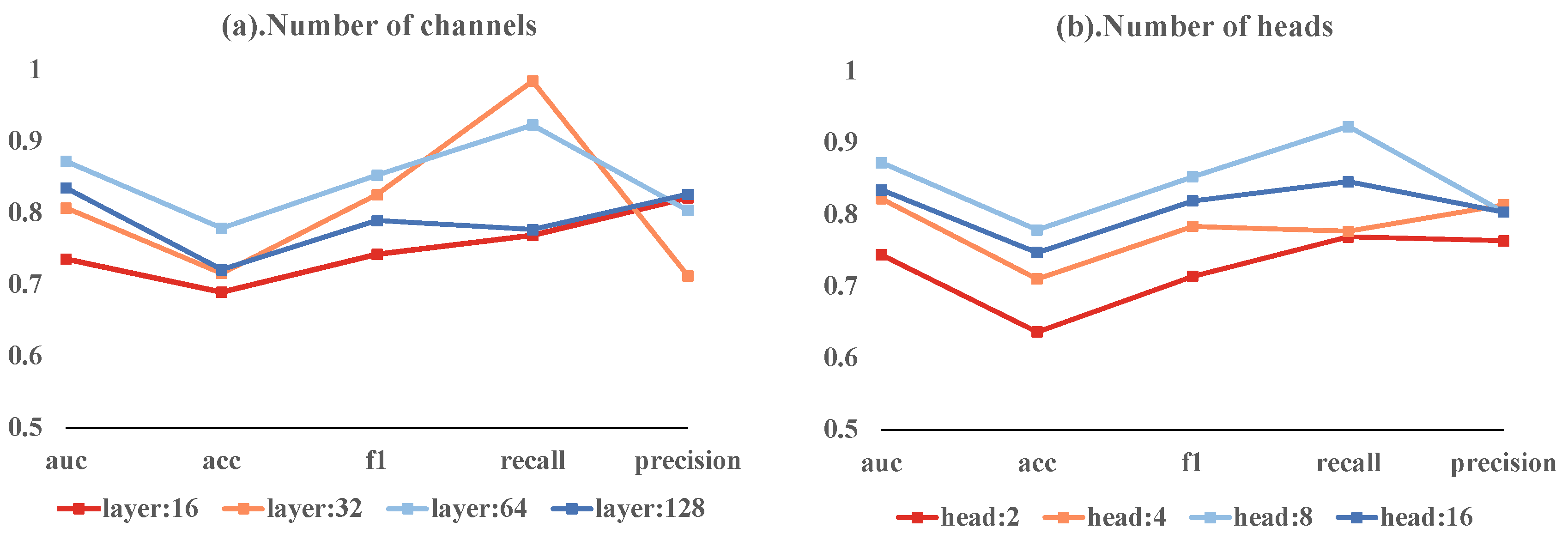
Our ablation study investigated the effects of varying the number of channels and heads in a multi-head attention mechanism on model performance. The models with 16, 32, 64, and 128 channels achieved AUC-ROCs of 0.7359, 0.8071, 0.8724, and 0.8352, respectively. The 64-channel model had the highest accuracy at 0.7789, with the 128-channel model close behind at 0.7211. These models exhibited different F1 scores, recall rates, and precision values. Notably, the 32-channel model achieved the highest recall of 0.9846.
In terms of head counts, models with 2, 4, 8, and 16 heads achieved AUC-ROCs of 0.7442, 0.8224, 0.8724, and 0.8346, respectively. The 8-head model stood out with the highest accuracy of 0.7789 and the highest F1 score of 0.8529. It also had the highest recall at 0.9231, while the 4-head model reached the peak precision of 0.8139.
The most balanced model combined 64 hidden layer channels with 8 heads, achieving an AUC-ROC of 0.8724, accuracy of 0.7789, F1 score of 0.8529, recall of 0.9231, and precision of 0.8038. These results suggest that deviating from these optimal settings leads to reduced performance. These variations are depicted in Figure 4, emphasizing the importance of a balanced model architecture for effective predictions.
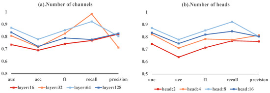
Figure 4.
Ablation study results showing the impact of different head counts and channel numbers on model performance.
6. Discussion
This study evaluated the effectiveness of our method in predicting the responses of bladder cancer patients to neoadjuvant therapy using transcriptomic data. The Boruta algorithm used in this study initially identified genes linked to treatment outcomes. Our Boruta-80 model outperformed other versions, highlighting the importance of choosing relevant genes for increased model precision. This aligns with Occam’s Razor, suggesting that simpler models often generalize better while maintaining strong predictive power. However, in the field of biomedical research, considering the complexity of biological processes, the complexity of models is sometimes necessary [47].
We underscore the importance of integrating biological insights with network-based ML techniques in clinical decision-making for neoadjuvant therapies. A major challenge we faced was applying traditional machine-learning methods to complex genetic data, which often led to issues of overfitting or underfitting [48,49]. In our experiment, despite SVM exhibiting commendable precision (), it may fail to accurately identify all patients who could benefit from the treatment, therefore increasing the risk of misdiagnosis. This concern is further demonstrated by the low recall rate of SVM (), reflecting the potential for overlooking patients who would respond positively to the therapy. Additionally, the clinical application of artificial intelligence in the medical field faces challenges in terms of transparency and reproducibility [50]. Studies in the domain of radiomics machine-learning (employing methods to analyze CT and MRI data for disease prediction, akin to our focus on small, high-dimensional datasets for clinical prognosis) have shown that single random train-test splits may lead to unreliable model performance assessments [51]. This highlights the importance of employing cross-validation or other techniques for a more accurate evaluation of model generalization capabilities. Against this backdrop, our proposed MVMSGAT model demonstrates more promising results compared to traditional models. Across multiple performance metrics, including AUC-ROC (), accuracy (), F1 score (), recall (), and precision (), MVMSGAT generally outperforms SVM, DT, RF, GBDT, GAT, MSGAT. Incorporating biological prior knowledge provides a significant benefit: models such as GAT, MSGAT, and MVMSGAT demonstrate smaller standard deviations in five-fold cross-validation, suggesting more stable results. This stability, particularly in contrast to traditional data-driven machine-learning methods, is likely because graph-based models handle high-dimensional data more effectively and are better at capturing complex biomarker interactions. These interactions, such as gene-gene interactions or protein pathways, are crucial for understanding disease mechanisms. Instead of relying solely on data-driven patterns like traditional methods, these models integrate biological insights, potentially enhancing their analytical capabilities and yielding more reliable and consistent results [52].
The primary goal of neoadjuvant therapies is shrinking tumor size to improve surgical outcomes, eliminating micro-metastases to lower recurrence risk, and assessing tumor response to specific treatments [53,54]. In this setting, the MVMSGAT model excels. Its recall rate is the second highest among its counterparts. More importantly, it leads in critical metrics like AUC-ROC, Accuracy, and F1 Score. This model’s overall effectiveness ensures it accurately identifies many patients likely to benefit from treatment. It reduces false diagnoses and ensures that all eligible patients receive the right care. This accurate and comprehensive diagnostic capability is vital for the success of neoadjuvant therapies, significantly affecting patient prognosis and quality of life. The effectiveness and accuracy of the MVMSGAT model mainly come from two areas: its handling of multi-scale gene cluster features and the integration of graph inputs from various biological perspectives at the mRNA level. Traditional methods for graph-level prediction often use simple readout operations, like averaging or maximizing node values, which can lead to a loss of important structural information. The MVMSGAT model overcomes this with multi-scale pooling and hierarchical pooling operations. These allow for data integration at different levels of detail, preserving crucial structural information. The model’s ability to combine gene clusters at multiple scales captures finer biological details and biomarker features. Additionally, by specifically integrating gene co-expression networks and protein–protein interaction networks at the mRNA level, the MVMSGAT model offers a more thorough analysis of the biological processes involved in new adjuvant therapies. This combination of technical advancements and focus on mRNA-level interactions greatly improves the model’s performance in complex biological studies. This aligns well with the goals of neoadjuvant therapies to enhance patient outcomes.
Furthermore, the relevance of selected genes, like VCAM1, IL6R, CD46, and ATF3, is supported by clinical research. VCAM1, a cell adhesion molecule, is upregulated in several cancers, including bladder cancer. It plays a crucial role in tumor cell adhesion, migration, and invasion, possibly interacting with immune cells in the tumor microenvironment [55,56]. IL6R, a cytokine receptor, regulates immune and inflammatory responses. Its activation in bladder cancer may encourage tumor growth and progression by affecting cell survival and proliferation [57,58,59]. CD46, regulating immune responses, shows abnormal expression in some cancers and relates to the aggressiveness and prognosis of bladder cancer [60]. ATF3, a stress-responsive transcription factor, is activated in various cell stress and pathological conditions. It may regulate cellular stress responses, affecting the survival and death of tumor cells in bladder cancer [61,62]. These insights shed light on the complex biological processes in bladder cancer and validate the MVMSGAT model’s ability to accurately predict patient responses to therapy.
6.1. Limitations
Although our method has demonstrated potential in predicting the efficacy of neoadjuvant therapy for bladder cancer, it is crucial to acknowledge its limitations for a comprehensive understanding. A significant limitation of our study is the reliance on a relatively small dataset, comprising only 210 samples. This size limits the statistical power of our analysis and may not adequately represent the diversity in bladder cancer stages and subtypes, potentially impacting the robustness and generalizability of our findings to different patient populations. The inherent biases present in publicly available datasets, such as the potential over-representation of certain demographic groups or under-representation of specific bladder cancer subtypes, further exacerbate this issue. Additionally, our study’s methodological framework, particularly regarding threshold settings, warrants careful consideration. This includes not only the feature importance threshold established for the dataset but also the threshold settings used in constructing the network models, which might vary significantly across different bladder cancer datasets due to variations in clinical characteristics and treatment responses. These thresholds, while effective within the context of our current study, might not be directly applicable to other datasets or different stages and subtypes of bladder cancer. This limitation is crucial as it affects both the selection of significant features and the structure of the network models, which are integral to our method’s performance. The specificity of these thresholds to our dataset underscores the need for caution when extrapolating our results beyond the current study’s scope.
6.2. Future Work
In terms of future work, addressing these limitations is paramount. First, expanding the dataset size is essential. Incorporating a larger and more diverse sample pool of bladder cancer patients would help mitigate the biases and enhance the generalizability of our model. This expansion would also provide a more robust foundation for validating the feature importance and network model thresholds across various types of bladder cancer data. Moreover, an exciting direction for future work is the integration of multi-omics data with artificial intelligence. Multi-omics approaches, which encompass genomics, proteomics, metabolomics, and more, offer a holistic view of the biological mechanisms underlying bladder cancer [63,64]. Leveraging such comprehensive data can uncover deeper insights into bladder cancer biology and potentially lead to more accurate and personalized treatment strategies. The combination of multi-omics data and AI has the potential to significantly advance our understanding of bladder cancer, enabling more effective and tailored interventions [65].
In conclusion, our study introduces a new precision medicine approach for bladder cancer treatment, combining multiview knowledge graphs with graph convolutional neural networks. This methodology has been thoroughly tested on the GEO dataset using a five-fold cross-validation, demonstrating excellent performance with an AUC-ROC of , accuracy of , F1 score of , recall of , and precision of . These results outperform most metrics of other methods and underscore the benefits of integrating graph convolutional neural networks with biological knowledge in predicting treatment outcomes. Furthermore, the alignment of selected genes with clinical insights confirms the reliability of our approach. Although these findings are promising for the prediction of neoadjuvant therapy efficacy in bladder cancer, the need for further research is evident. Future studies involving larger and more diverse datasets, as well as the exploration of multi-omics data in conjunction with AI, are crucial. These steps, challenging as they may be and requiring interdisciplinary collaboration and funding, are essential to enhance the reliability and applicability of our approach and to achieve significant advancements in personalized medicine for bladder cancer treatment.
7. Conclusions
In our research, we introduced MVMSGAT, a new predictive model specifically designed to accurately predict bladder cancer patients’ responses to neoadjuvant therapy. Our approach began with the Boruta algorithm to identify key genes from transcriptomic data. The central innovation of MVMSGAT is its integration of biological prior knowledge with a multiview knowledge graph, forming a detailed and effective analytical framework. This integration is pivotal, allowing the model to process complex biological information efficiently, therefore significantly boosting its precision and reliability. Tested through five-fold cross-validation on two datasets from the GEO database, encompassing a total of 210 bladder cancer cases, MVMSGAT demonstrated superior performance in most metrics compared to existing methods. This showcases its substantial potential in advancing personalized treatment and precision medicine for bladder cancer. Additionally, the congruence of the selected genes with clinical insights underlines the model’s applicability and relevance in the context of bladder cancer therapy.
Supplementary Materials
The following supporting information can be downloaded at: https://www.mdpi.com/article/10.3390/app14020669/s1, Table S1: Clinical information of patients; Table S2: Expression data from the GSE169455 and GSE69795 datasets; Table S3: The detailed gene names under different Boruta selection thresholds.
Author Contributions
Conceptualization, X.L. and X.C.; methodology, X.L.; software, X.L.; validation, X.L., X.C. and Y.Y.; formal analysis, X.L.; data curation, X.L.; writing—original draft preparation, X.L.; writing—review and editing, X.L. and X.C.; visualization, X.L.; funding acquisition, Y.Y. All authors have read and agreed to the published version of the manuscript.
Funding
This work was supported by the Sichuan Province Key Research and Development Project [Project No. RZHZ2022004].
Institutional Review Board Statement
Not applicable.
Informed Consent Statement
Not applicable.
Data Availability Statement
Data are contained within the article and Supplementary Materials.
Conflicts of Interest
The authors declare no conflict of interest.
Abbreviations
The following abbreviations are used in this manuscript:
| NMIBC | Non-Muscle-Invasive Bladder Cancer |
| MIBC | Muscle-Invasive Bladder Cancer |
| ML | Machine Learning |
| GCN | Graph Convolutional Networks |
| SVM | Support Vector Machines |
| DEGs | differentially expressed genes |
| pCR | pathological complete response |
| HCC | Hepatocellular Carcinoma |
| GEO | Gene Expression Omnibus |
| MZSA | Maximum Z score among shadow attributes |
| PPI | Protein–Protein Interaction |
| CR | Complete Response |
| PR | Partial Response |
| SD | Stable Disease |
| PD | Progressive Disease |
| DT | Decision Trees |
| RF | Random Forest |
| GBDT | Gradient Boosting Decision Trees |
| GAT | Graph Attention Networks |
| MSGAT | Multi-Scale Graph Attention Networks |
| MVMSGAT | Multiview Multi-Scale Graph Attention Networks |
| VCAM1 | Vascular Cell Adhesion Molecule 1 |
| IL6R | Interleukin 6 Receptor |
| ATF3 | Activating Transcription Factor 3 |
References
- Siegel, R.L.; Miller, K.D.; Wagle, N.S.; Jemal, A. Cancer statistics, 2023. CA Cancer J. Clin. 2023, 73, 17–48. [Google Scholar] [CrossRef] [PubMed]
- Prasad, S.M.; DeCastro, G.J.; Steinberg, G.D. Urothelial carcinoma of the bladder: Definition, treatment and future efforts. Nat. Rev. Urol. 2011, 8, 631–642. [Google Scholar] [CrossRef] [PubMed]
- da Costa, J.B.; Gibb, E.A.; Nykopp, T.K.; Mannas, M.; Wyatt, A.W.; Black, P.C. Molecular tumor heterogeneity in muscle invasive bladder cancer: Biomarkers, subtypes, and implications for therapy. Urol. Oncol. Semin. Orig. Investig. 2022, 40, 287–294. [Google Scholar] [CrossRef]
- Chin, L.; Andersen, J.N.; Futreal, P.A. Cancer genomics: From discovery science to personalized medicine. Nat. Med. 2011, 17, 297–303. [Google Scholar] [CrossRef] [PubMed]
- Alqahtani, A.; Alsubai, S.; Binbusayyis, A.; Sha, M.; Gumaei, A.; Zhang, Y.D. Prediction of Urinary Tract Infection in IoT-Fog Environment for Smart Toilets Using Modified Attention-Based ANN and Machine Learning Algorithms. Appl. Sci. 2023, 13, 5860. [Google Scholar] [CrossRef]
- Zhang, Y.; Hong, J.; Chen, S. Medical Big Data and Artificial Intelligence for Healthcare. Appl. Sci. 2023, 13, 3745. [Google Scholar] [CrossRef]
- Shen, J.; Qi, L.; Zou, Z.; Du, J.; Kong, W.; Zhao, L.; Wei, J.; Lin, L.; Ren, M.; Liu, B. Identification of a novel gene signature for the prediction of recurrence in HCC patients by machine learning of genome-wide databases. Sci. Rep. 2020, 10, 4435. [Google Scholar] [CrossRef]
- Wiesweg, M.; Mairinger, F.; Reis, H.; Goetz, M.; Kollmeier, J.; Misch, D.; Stephan-Falkenau, S.; Mairinger, T.; Walter, R.F.; Hager, T. Machine learning reveals a PD-L1–independent prediction of response to immunotherapy of non-small cell lung cancer by gene expression context. Eur. J. Cancer 2020, 140, 76–85. [Google Scholar] [CrossRef]
- Taghizadeh, E.; Heydarheydari, S.; Saberi, A.; JafarpoorNesheli, S.; Rezaeijo, S.M. Breast cancer prediction with transcriptome profiling using feature selection and machine learning methods. BMC Bioinform. 2022, 23, 410. [Google Scholar] [CrossRef]
- Li, Y.; Wu, F.X.; Ngom, A. A review on machine learning principles for multi-view biological data integration. Briefings Bioinform. 2018, 19, 325–340. [Google Scholar] [CrossRef]
- Crawford, J.; Greene, C.S. Incorporating biological structure into machine learning models in biomedicine. Curr. Opin. Biotechnol. 2020, 63, 126–134. [Google Scholar] [CrossRef] [PubMed]
- Alber, M.; Buganza Tepole, A.; Cannon, W.R.; De, S.; Dura-Bernal, S.; Garikipati, K.; Karniadakis, G.; Lytton, W.W.; Perdikaris, P.; Petzold, L.; et al. Integrating machine learning and multiscale modeling—perspectives, challenges, and opportunities in the biological, biomedical, and behavioral sciences. NPJ Digit. Med. 2019, 2, 115. [Google Scholar] [CrossRef] [PubMed]
- Mudiyanselage, T.B.; Lei, X.; Senanayake, N.; Zhang, Y.; Pan, Y. Predicting CircRNA disease associations using novel node classification and link prediction models on graph convolutional networks. Methods 2022, 198, 32–44. [Google Scholar] [CrossRef] [PubMed]
- Choi, W.; Lee, H. Identifying disease-gene associations using a convolutional neural network-based model by embedding a biological knowledge graph with entity descriptions. PLoS ONE 2021, 16, e0258626. [Google Scholar] [CrossRef] [PubMed]
- Font, A.; Taron, M.; Gago, J.; Costa, C.; Sánchez, J.; Carrato, C.; Mora, M.; Celiz, P.; Perez, L.; Rodríguez, D.; et al. BRCA1 mRNA expression and outcome to neoadjuvant cisplatin-based chemotherapy in bladder cancer. Ann. Oncol. 2011, 22, 139–144. [Google Scholar] [CrossRef]
- Van Allen, E.M.; Mouw, K.W.; Kim, P.; Iyer, G.; Wagle, N.; Al-Ahmadie, H.; Zhu, C.; Ostrovnaya, I.; Kryukov, G.V.; O’Connor, K.W.; et al. Somatic ERCC2 mutations correlate with cisplatin sensitivity in muscle-invasive urothelial carcinoma. Cancer Discov. 2014, 4, 1140–1153. [Google Scholar] [CrossRef]
- Groenendijk, F.H.; de Jong, J.; van de Putte, E.E.F.; Michaut, M.; Schlicker, A.; Peters, D.; Velds, A.; Nieuwland, M.; van den Heuvel, M.M.; Kerkhoven, R.M.; et al. ERBB2 mutations characterize a subgroup of muscle-invasive bladder cancers with excellent response to neoadjuvant chemotherapy. Eur. Urol. 2016, 69, 384–388. [Google Scholar] [CrossRef]
- Takata, R.; Katagiri, T.; Kanehira, M.; Tsunoda, T.; Shuin, T.; Miki, T.; Namiki, M.; Kohri, K.; Matsushita, Y.; Fujioka, T.; et al. Predicting response to methotrexate, vinblastine, doxorubicin, and cisplatin neoadjuvant chemotherapy for bladder cancers through genome-wide gene expression profiling. Clin. Cancer Res. 2005, 11, 2625–2636. [Google Scholar] [CrossRef]
- Takata, R.; Katagiri, T.; Kanehira, M.; Shuin, T.; Miki, T.; Namiki, M.; Kohri, K.; Tsunoda, T.; Fujioka, T.; Nakamura, Y. Validation study of the prediction system for clinical response of M-VAC neoadjuvant chemotherapy. Cancer Sci. 2007, 98, 113–117. [Google Scholar] [CrossRef]
- Ng, S.; Masarone, S.; Watson, D.; Barnes, M.R. The benefits and pitfalls of machine learning for biomarker discovery. Cell Tissue Res. 2023, 394, 17–31. [Google Scholar] [CrossRef]
- Huang, C.; Clayton, E.A.; Matyunina, L.V.; McDonald, L.D.; Benigno, B.B.; Vannberg, F.; McDonald, J.F. Machine learning predicts individual cancer patient responses to therapeutic drugs with high accuracy. Sci. Rep. 2018, 8, 16444. [Google Scholar] [CrossRef]
- Lu, W.; Fu, D.; Kong, X.; Huang, Z.; Hwang, M.; Zhu, Y.; Chen, L.; Jiang, K.; Li, X.; Wu, Y.; et al. FOLFOX treatment response prediction in metastatic or recurrent colorectal cancer patients via machine learning algorithms. Cancer Med. 2020, 9, 1419–1429. [Google Scholar] [CrossRef] [PubMed]
- Sayaman, R.W.; Wolf, D.M.; Yau, C.; Wulfkuhle, J.; Petricoin, E.; Brown-Swigart, L.; Asare, S.M.; Hirst, G.L.; Sit, L.; O’Grady, N.; et al. Abstract P1-21-08: Application of machine learning to elucidate the biology predicting response in the I-SPY 2 neoadjuvant breast cancer trial. Cancer Res. 2020, 80, P1-21-08. [Google Scholar] [CrossRef]
- Chen, D.; Liu, J.; Zang, L.; Xiao, T.; Zhang, X.; Li, Z.; Zhu, H.; Gao, W.; Yu, X. Integrated machine learning and bioinformatic analyses constructed a novel stemness-related classifier to predict prognosis and immunotherapy responses for hepatocellular carcinoma patients. Int. J. Biol. Sci. 2022, 18, 360. [Google Scholar] [CrossRef] [PubMed]
- Baptista, D.; Ferreira, P.G.; Rocha, M. Deep learning for drug response prediction in cancer. Briefings Bioinform. 2021, 22, 360–379. [Google Scholar] [CrossRef]
- Chang, Y.; Park, H.; Yang, H.J.; Lee, S.; Lee, K.Y.; Kim, T.S.; Jung, J.; Shin, J.M. Cancer drug response profile scan (CDRscan): A deep learning model that predicts drug effectiveness from cancer genomic signature. Sci. Rep. 2018, 8, 8857. [Google Scholar] [CrossRef]
- Xia, F.; Shukla, M.; Brettin, T.; Garcia-Cardona, C.; Cohn, J.; Allen, J.E.; Maslov, S.; Holbeck, S.L.; Doroshow, J.H.; Evrard, Y.A.; et al. Predicting tumor cell line response to drug pairs with deep learning. BMC Bioinform. 2018, 19, 71–79. [Google Scholar] [CrossRef]
- Chiu, Y.C.; Chen, H.I.H.; Zhang, T.; Zhang, S.; Gorthi, A.; Wang, L.J.; Huang, Y.; Chen, Y. Predicting drug response of tumors from integrated genomic profiles by deep neural networks. BMC Med Genom. 2019, 12, 143–155. [Google Scholar]
- Guyon, I.; Elisseeff, A. An introduction to variable and feature selection. J. Mach. Learn. Res. 2003, 3, 1157–1182. [Google Scholar]
- Kursa, M.B.; Rudnicki, W.R. Feature selection with the Boruta package. J. Stat. Softw. 2010, 36, 1–13. [Google Scholar] [CrossRef]
- Kursa, M.B.; Jankowski, A.; Rudnicki, W.R. Boruta—A system for feature selection. Fundam. Informaticae 2010, 101, 271–285. [Google Scholar] [CrossRef]
- Tang, R.; Zhang, X. CART decision tree combined with Boruta feature selection for medical data classification. In Proceedings of the 2020 5th IEEE International Conference on Big Data Analytics (ICBDA), Xiamen, China, 8–11 May 2020; pp. 80–84. [Google Scholar]
- Kumar, S.S.; Shaikh, T. Empirical evaluation of the performance of feature selection approaches on random forest. In Proceedings of the 2017 International Conference on Computer and Applications (ICCA), Doha, Qatar, 6–7 September 2017; pp. 227–231. [Google Scholar]
- Yang, Y.; Han, L.; Yuan, Y.; Li, J.; Hei, N.; Liang, H. Gene co-expression network analysis reveals common system-level properties of prognostic genes across cancer types. Nat. Commun. 2014, 5, 3231. [Google Scholar] [CrossRef] [PubMed]
- Zhang, B.; Horvath, S. A general framework for weighted gene co-expression network analysis. Stat. Appl. Genet. Mol. Biol. 2005, 4, 17. [Google Scholar] [CrossRef] [PubMed]
- Stelzl, U.; Worm, U.; Lalowski, M.; Haenig, C.; Brembeck, F.H.; Goehler, H.; Stroedicke, M.; Zenkner, M.; Schoenherr, A.; Koeppen, S. A human protein-protein interaction network: A resource for annotating the proteome. Cell 2005, 122, 957–968. [Google Scholar] [CrossRef] [PubMed]
- Rual, J.F.; Venkatesan, K.; Hao, T.; Hirozane-Kishikawa, T.; Dricot, A.; Li, N.; Berriz, G.F.; Gibbons, F.D.; Dreze, M.; Ayivi-Guedehoussou, N. Towards a proteome-scale map of the human protein–protein interaction network. Nature 2005, 437, 1173–1178. [Google Scholar] [CrossRef] [PubMed]
- Mering, C.v.; Huynen, M.; Jaeggi, D.; Schmidt, S.; Bork, P.; Snel, B. STRING: A database of predicted functional associations between proteins. Nucleic Acids Res. 2003, 31, 258–261. [Google Scholar] [CrossRef] [PubMed]
- Dahiya, S.; Saini, V.; Kumar, P.; Kumar, A. Protein-protein interaction network analyses of human WNT proteins involved in neural development. Bioinformation 2019, 15, 307. [Google Scholar] [CrossRef]
- Xu, K.; Hu, W.; Leskovec, J.; Jegelka, S. How powerful are graph neural networks? arXiv 2018, arXiv:1810.00826. [Google Scholar]
- Veličković, P.; Cucurull, G.; Casanova, A.; Romero, A.; Lio, P.; Bengio, Y. Graph attention networks. arXiv 2017, arXiv:1710.10903. [Google Scholar]
- Cangea, C.; Veličković, P.; Jovanović, N.; Kipf, T.; Liò, P. Towards sparse hierarchical graph classifiers. arXiv 2018, arXiv:1811.01287. [Google Scholar]
- Knyazev, B.; Taylor, G.W.; Amer, M. Understanding attention and generalization in graph neural networks. Adv. Neural Inf. Process. Syst. 2019, 32, 4202–4212. [Google Scholar]
- Sjödahl, G.; Abrahamsson, J.; Holmsten, K.; Bernardo, C.; Chebil, G.; Eriksson, P.; Johansson, I.; Kollberg, P.; Lindh, C.; Lövgren, K. Different responses to neoadjuvant chemotherapy in urothelial carcinoma molecular subtypes. Eur. Urol. 2022, 81, 523–532. [Google Scholar] [CrossRef] [PubMed]
- McConkey, D.J.; Choi, W.; Shen, Y.; Lee, I.L.; Porten, S.; Matin, S.F.; Kamat, A.M.; Corn, P.; Millikan, R.E.; Dinney, C. A prognostic gene expression signature in the molecular classification of chemotherapy-naive urothelial cancer is predictive of clinical outcomes from neoadjuvant chemotherapy: A phase 2 trial of dose-dense methotrexate, vinblastine, doxorubicin, and cisplatin with bevacizumab in urothelial cancer. Eur. Urol. 2016, 69, 855–862. [Google Scholar] [PubMed]
- Leek, J.T.; Johnson, W.E.; Parker, H.S.; Jaffe, A.E.; Storey, J.D. The sva package for removing batch effects and other unwanted variation in high-throughput experiments. Bioinformatics 2012, 28, 882–883. [Google Scholar] [CrossRef] [PubMed]
- Greener, J.G.; Kandathil, S.M.; Moffat, L.; Jones, D.T. A guide to machine learning for biologists. Nat. Rev. Mol. Cell Biol. 2022, 23, 40–55. [Google Scholar] [CrossRef] [PubMed]
- Almugren, N.; Alshamlan, H. A survey on hybrid feature selection methods in microarray gene expression data for cancer classification. IEEE Access 2019, 7, 78533–78548. [Google Scholar] [CrossRef]
- Momeni, Z.; Hassanzadeh, E.; Abadeh, M.S.; Bellazzi, R. A survey on single and multi omics data mining methods in cancer data classification. J. Biomed. Informatics 2020, 107, 103466. [Google Scholar] [CrossRef]
- Haibe-Kains, B.; Adam, G.A.; Hosny, A.; Khodakarami, F.; Massive Analysis Quality Control (MAQC) Society Board of Directors; Waldron, L.; Wang, B.; McIntosh, C.; Goldenberg, A.; Kundaje, A.; et al. Transparency and reproducibility in artificial intelligence. Nature 2020, 586, E14–E16. [Google Scholar] [CrossRef]
- An, C.; Park, Y.W.; Ahn, S.S.; Han, K.; Kim, H.; Lee, S.K. Radiomics machine learning study with a small sample size: Single random training-test set split may lead to unreliable results. PLoS ONE 2021, 16, e0256152. [Google Scholar] [CrossRef]
- Mohamed, S.K.; Nováček, V.; Nounu, A. Discovering protein drug targets using knowledge graph embeddings. Bioinformatics 2020, 36, 603–610. [Google Scholar] [CrossRef]
- Nguyen, D.P.; Thalmann, G.N. Contemporary update on neoadjuvant therapy for bladder cancer. Nat. Rev. Urol. 2017, 14, 348–358. [Google Scholar] [CrossRef] [PubMed]
- Hermans, T.J.; Voskuilen, C.S.; van der Heijden, M.S.; Schmitz-Dräger, B.J.; Kassouf, W.; Seiler, R.; Kamat, A.M.; Grivas, P.; Kiltie, A.E.; Black, P.C.; et al. Neoadjuvant treatment for muscle-invasive bladder cancer: The past, the present, and the future. Urol. Oncol. Semin. Orig. Investig. 2018, 36, 413–422. [Google Scholar] [CrossRef] [PubMed]
- Chen, Q.; Massagué, J. Molecular pathways: VCAM-1 as a potential therapeutic target in metastasis. Clin. Cancer Res. 2012, 18, 5520–5525. [Google Scholar] [CrossRef]
- Wu, T.C. The role of vascular cell adhesion molecule-1 in tumor immune evasion. Cancer Res. 2007, 67, 6003–6006. [Google Scholar] [CrossRef]
- Wei, H. Interleukin 6 signaling maintains the stem-like properties of bladder cancer stem cells. Transl. Cancer Res. 2019, 8, 557. [Google Scholar] [CrossRef] [PubMed]
- Chen, M.F.; Lin, P.Y.; Wu, C.F.; Chen, W.C.; Wu, C.T. IL-6 expression regulates tumorigenicity and correlates with prognosis in bladder cancer. PLoS ONE 2013, 8, e61901. [Google Scholar] [CrossRef]
- Goulet, C.R.; Champagne, A.; Bernard, G.; Vandal, D.; Chabaud, S.; Pouliot, F.; Bolduc, S. Cancer-associated fibroblasts induce epithelial–mesenchymal transition of bladder cancer cells through paracrine IL-6 signalling. BMC Cancer 2019, 19, 137. [Google Scholar] [CrossRef] [PubMed]
- Zeng, J.; Xu, H.; Huang, C.; Sun, Y.; Xiao, H.; Yu, G.; Zhou, H.; Zhang, Y.; Yao, W.; Xiao, W.; et al. CD46 splice variant enhances translation of specific mRNAs linked to an aggressive tumor cell phenotype in bladder cancer. Mol. Ther.-Nucleic Acids 2021, 24, 140–153. [Google Scholar] [CrossRef]
- Yuan, X.; Yu, L.; Li, J.; Xie, G.; Rong, T.; Zhang, L.; Chen, J.; Meng, Q.; Irving, A.T.; Wang, D.; et al. ATF3 suppresses metastasis of bladder cancer by regulating gelsolin-mediated remodeling of the actin cytoskeleton. Cancer Res. 2013, 73, 3625–3637. [Google Scholar] [CrossRef]
- Xie, H.; Wang, M.; Yu, H.; Wang, H.; Ding, L.; Wang, R.; Luo, W.; Lu, Z.; Zheng, Q.; Ren, L.; et al. METTL1 drives tumor progression of bladder cancer via degrading ATF3 mRNA in an m7G-modified miR-760-dependent manner. Cell Death Discov. 2022, 8, 458. [Google Scholar] [CrossRef]
- Holzinger, A.; Haibe-Kains, B.; Jurisica, I. Why imaging data alone is not enough: AI-based integration of imaging, omics, and clinical data. Eur. J. Nucl. Med. Mol. Imaging 2019, 46, 2722–2730. [Google Scholar] [CrossRef] [PubMed]
- Reel, P.S.; Reel, S.; Pearson, E.; Trucco, E.; Jefferson, E. Using machine learning approaches for multi-omics data analysis: A review. Biotechnol. Adv. 2021, 49, 107739. [Google Scholar] [CrossRef] [PubMed]
- Subramanian, I.; Verma, S.; Kumar, S.; Jere, A.; Anamika, K. Multi-omics data integration, interpretation, and its application. Bioinform. Biol. Insights 2020, 14, 1177932219899051. [Google Scholar] [CrossRef] [PubMed]


Disclaimer/Publisher’s Note: The statements, opinions and data contained in all publications are solely those of the individual author(s) and contributor(s) and not of MDPI and/or the editor(s). MDPI and/or the editor(s) disclaim responsibility for any injury to people or property resulting from any ideas, methods, instructions or products referred to in the content. |
© 2024 by the authors. Licensee MDPI, Basel, Switzerland. This article is an open access article distributed under the terms and conditions of the Creative Commons Attribution (CC BY) license (https://creativecommons.org/licenses/by/4.0/).