The Temperature Field Prediction and Estimation of Ti-Al Alloy Twin-Wire Plasma Arc Additive Manufacturing Using a One-Dimensional Convolution Neural Network

Abstract

Plasma arc deposition as an additive manufacturing technology has unique advantages for producing parts with complex shapes through layer-by-layer deposition. It is critical to predict and control the temperature field during the production process due to the temperature distribution and gradients determining the properties and performance of the part. Numerical simulation approaches, such as the finite element method, which provides a large amount of data for machine learning modeling, thus reducing the overhead of experimental measurements, are widely used in machine learning. In this paper, we propose a neural network combined finite element method and process prediction workflow. A one-dimensional convolutional neural network model for predicting 2D temperature distribution is developed by training the collected data on the planar temperature field of titanium–aluminum twin-wire plasma arc additive manufacturing and the finite element method. The results show that the predicted temperature mean square error is only 0.5, with less than a 20 °C error in peak temperature and a relative error below 1%. The proposed transfer learning method achieves the same training loss and is 500 iterations faster than basic training, which improves the training speed by 25%. The current study confirms the accurate performance of the ML model and the effectiveness of the optimization method.

1. Introduction

Plasma arc additive manufacturing (PAAM) technology utilizes an electric arc to melt powder or filament material and solidify it on a substrate or previous layer to create parts via layer-by-layer deposition [1]. It has the superior ability to directly print complex geometrical parts compared to traditional manufacturing techniques [2]. Titanium–aluminum alloys have the merits of material properties, while their usage is constrained due to their weak ductility at room temperature [3]. Therefore, additive technology like PAAW serves as an ideal process for manufacturing Ti-Al alloys [4]. A huge temperature gradient exists near the melt pool during the deposition process, which leads to significant thermal residual stress and deformation that affect the mechanical properties of the part [5].

The temperature distribution during the deposition process is a key factor in determining the quality of the printed components. In recent years, researchers have studied these temperature distribution features considering the factors of the heat source mode, print material delivery form, and print path [6,7,8]. At the same time, it is common to use finite element methods instead of experiments to study the characterizations of the deposition process [9]. The use of this method possesses advantages such as cost savings and reduced difficulty in parameter measurement [10]. However, trade-offs need to be made between computational accuracy and computational time [11,12].

With the explosive growth of machine learning research, many scholars have tried to use in situ parameters to predict experiment results. Zhang et al. [13] predicted the producing quality by using molten pool, plume, and spatter images obtained from a high-speed camera. Shevchik et al. [14] used acoustic signals to determine the producing quality during the deposition process. Montazeri et al. [15] collected spectral data and used neural networks, support vector machines, and linear discriminant analysis to predict the manufacturing quality. Xie et al. [16] collected infrared temperature data and used them to predict mechanical properties such as the maximum tensile strength of a component.

Many scholars have found that the cost of data collection can be reduced through a numerical simulation approach. Chowdhury et al. [17] used an artificial neural network model that predicted thermal deformation by extracting the deformation nodes generated by the finite element model. Roy et al. [18] used a machine learning algorithm to propose a fast surrogate model to replace the traditional numerical simulation methods for acquiring temperature cycle features during the deposition process. Data-driven methods can generate hundreds of thousands of data for further analysis [19], which are difficult to reach through experiments. Raissi et al. [20,21] proposed a neural network approach for solving partial differential equations, which benefited from the popularization of the concept of Automatic Differentiation (AD) [22] in ML algorithms. Lu et al. [23] applied such physics-informed neural networks (PINNs) to solve the partial differential equations of heat conduction and compared them with the traditional FEM, achieving ideal results. Li et al. [24] proposed an innovation in the structure of neural networks by combining residual block with PINN and achieved great results. However, restricted to the structure itself, this method can only perform point-to-point prediction, and there exists the problem of solving the partial differential equation logically under the physical law for 2D scenes [23]. To fit practical applications, ML approaches have also been used to investigate the effect of the deposition path on heat accumulation [19]. Ren et al. [25] summarized previous research results and used model predictions to guide a metal component printing process, which achieved the expected results. With the continuous progress of ML algorithms, many new structures of neural networks have been proposed to predict the temperature field of the deposition process [26,27,28].

To predict the temperature field and control the appearance of defects such as cracks during the deposition process [29,30], we constructed a novel one-dimensional convolutional neural network model for predicting the 2D temperature field during the deposition process by using one-dimensional feature data collected from the experiment, in which case, the feature is the temperature on the deposition path. Meanwhile, this paper proposes a neural network combined finite element method and process prediction workflow by combining a neural network, transfer training, and other methods. By constructing the FEM model, a large amount of training data is provided for the neural network model training, which ensures the robustness of the model. The proposal of transfer training dynamizes the training process of the model and improves the model prediction performance.

2. Datasets Building

2.1. Experiment Description

In our research [31,32], a TA2 titanium plate measuring 200 × 100 × 8 mm was used as the substrate. Titanium (ERTI-2) and aluminum (ER1100) feeding wires (both with diameters of 0.8 mm) were used as the deposition materials. The shielding gas was 99.9% Ar. Bottom-up deposition was performed using the PAAM to deposit 30 layers, each with an approximate thickness of 1 mm, as Figure 1a depicts. An infrared camera was used to collect the temperature field data of the molten pool and the substrate during the deposition process, as shown in Figure 1b.

Based on the substrate plane temperature field data during the deposition process of the first two layers of the experiment, we used FEM to reconstruct the 2D temperature distribution features of the plane and established the needed data set to train the neural network model. The fidelity of the neural network prediction results is guaranteed by the finite elements as well as the experimental data.

Table 1. Composition (at.%) of the Al alloy wire (ER1100).

	Si	Cu	Zn	Mn	Fe	Al
ER1100	0.03	0.02	0.013	0.003	0.18	Bal

and

Table 2. Composition (at.%) of the Ti alloy wire (ERTI-2) and the substrate (TA2).

	O	Fe	N	C	H	Ti
ERTI-2	0.08–0.16	0.12	0.015	0.03	0.008	Bal
TA2	0.25	0.3	0.05	0.1	0.015	Bal

show the elemental composition of the wire and the substrate.

2.2. Finite Element Method Description

Based on Fourier’s law, the general form of the heat transfer equation can be defined as:

$$\rho c\frac{\partial T}{\partial t}=\frac{\partial }{\partial x} \left(k_x\frac{\partial T}{\partial x}\right)+\frac{\partial }{\partial y} \left(k_y\frac{\partial T}{\partial y}\right)+\frac{\partial }{\partial z} \left(k_z\frac{\partial T}{\partial z}\right)+Q$$

(1)

where $\rho$ is the material density, $c$ is the specific heat capacity, $T$ is the temperature, $t$ is the time, and $Q$ is the heat flux. In addition, the subscripts $x$, $y$, and $z$ denote the horizontal arc motion, the vertical arc motion, and the direction perpendicular to the $xy$ plane, respectively. Moreover, $k_x$, $k_y$, and $k_z$ are the thermal conductivities as a function of $T$ in the $x$, $y$, and $z$ directions, respectively. The Gaussian cylindrical heat source is chosen as the Q heat source formula, as shown in Equation (2).

$$Q\left(x,y, t\right)=\frac{3\eta P_{ }}{\pi r^2} ·\exp \left(\frac{-C{\left(x-\left(vt+x_0\right)\right)}^2-C{\left(y-y_0\right)}^2}{r^2}\right)$$

(2)

$C$ is the concentration of the heat source, $\eta$ is the energy absorptivity, $P$ is the laser power, and $r$ is the plasma arc radius. The ambient temperature was 25 °C. For the initial temperature of the substrate, 300 °C was used. The boundary condition in the model was the convection with the air, which can be expressed as:

$$-k\frac{\partial T}{\partial \overrightarrow{n}}=h\left(T-T_a\right)$$

(3)

where $h$ is the heat convection coefficient between the substrate and air, $T_a$ is the ambient air temperature, and $\overrightarrow{n}$ is the orientation vector at the substrate surface. In our FEM model, the geometry of the simulation domain was set to 50 mm × 50 mm × 5 mm, with a total of 83,603 nodes and 75,168 cells. The mesh size was uniformly set to 1 mm × 1 m.

Table 3. Manufacturing parameters and material properties in the experiment.

	Name	Units	Value
Manufacturing parameters	DC Current	A	90
	Voltage	V	80
	Welding speed	$\mathrm{mm}/\min$	90
Material properties	Density	${\mathrm{g} \mathrm{m}}^{-3}$	3.525
	Thermal conductivity	${\mathrm{W} \mathrm{m}}^{-1} {°\mathrm{C}}^{-1}$	$1.79e^{-6}{T}^2+4.77e^{-3}T+15.9$
	Enthalpy	${\mathrm{J} \mathrm{g}}^{-1} {°\mathrm{C}}^{-1}$	$3.01e^{-5}{T}^2+0.69T-92.9$

summarizes the other relevant parameters during the simulation. The simulation process was conducted by a solver based on the Lagrange–Galerkin finite element method.

We used a Python script to extract the temperature data for each node from the FEM results. We designed 13 groups of single-track deposition with different time steps and different heat source locations to enrich the dataset. Each group was divided by time steps, and more than 1000 cases of temperature fields under different deposition times were collected. In total, 11 of these groups were training sets and 2 groups were validation sets, which represented short and long deposition times, respectively, and were not involved in the training stage. The training set and validation set vary in the total time used in the deposition process. Considering that the manufacturing parameters were defined values, the dominant factor that determined the temperature features was the variation in heat accumulation, which can be noted as the deposition time in our research. Each training set and validation set shared different deposition times. The volume of the validation set was 15% of the total dataset. We normalized the values of the temperature to 0∼1 in order to train the neural network model efficiently. The training set for the model consisted of 2D temperature fields as the output and the 1D temperatures at the center path as the input. In this paper, we focused on the temperature variations in the melting stage of the deposition process, and the temperatures of the cooling stage were not considered.

3. Methodology

3.1. Basic Workflow

Figure 2 illustrates a complete working framework model, where the training work is divided into two parts: basic training and transfer training [33]. When training for a specific set of manufacturing parameters, the whole training process goes into the left side of the basic training process, where finite element methods are used to obtain and pre-process the input. After the training stage, the well-trained model parameters are saved. When new manufacturing features, such as print path, print material, and other process parameters, emerge, the training process enters the transfer training process. The saved model parameters can be utilized as the initial parameters to fine-tune the performance of the model. The training cost can be significantly reduced by the transfer training method without losing the accuracy [34]. Thus, the use of transfer training makes the training stage a dynamic process to adapt to different situations.

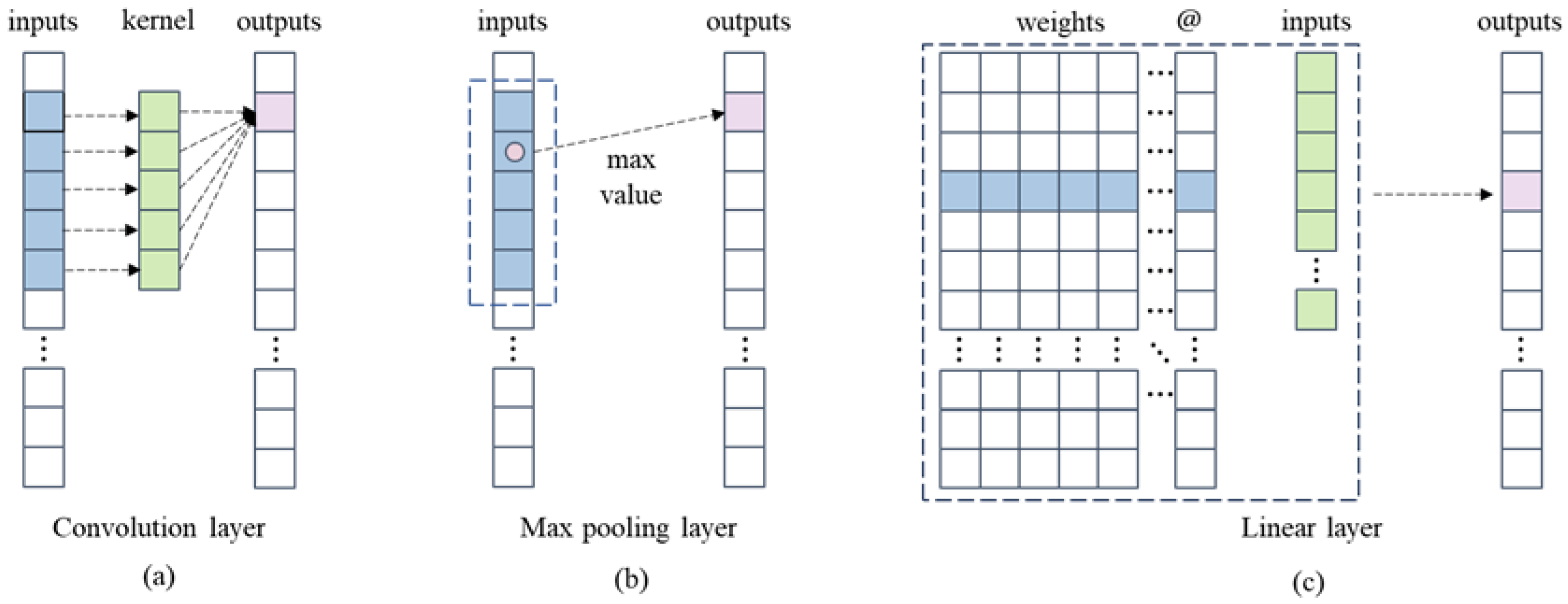
3.2. Architecture of the Conv1D Network

Figure 3 and Figure 4 provide illustrations of the network architecture and the operators used in each hidden layer. The model mainly consists of five groups of conv-blocks and the fully connected part. A conv-block can be subdivided into a convolutional layer and a linear layer.

When the training data are input into the convolutional layer, the convolution operation [35] is conducted. The convolution kernel scans through the input data and derives the eigenvalues, which can be expressed as:

$$a^l\left(l_{out},c_{out}\right)=w^l\left(c_{out},k\right)\ast a^{l-1}\left(l_{in},c_{in}\right)+b^l$$

(4)

where $w^l$ is the weight,$k$ is the kernel size, and $c_{out}$ is the number of output channels. $a^{l-1}$ is the input, $l_{in}$ is the length of the input, $c_{in}$ is the input channels, and $b$ is the bias. The length of the output, $l_{out}$, is computed from $l_{in}$ and $k$ using Equation (5).

$$l_{out}=\frac{l_{in}+2p-k}{s}+1$$

(5)

where p is the number of zero-padding and s is the size of stride. In our model, p = 2 and s = 1. The convolutional layer is followed by a pooling layer, which amplifies the data features following the logic of max-pooling [36]. Unlike the convolutional layer, there are no weights and biases in the pooling layer, only the input data are scanned, and the maximum value of each kernel is selected. After the convolution operator, the ReLU nonlinear operator is performed. The nonlinear operation is calculated as:

$$a^l=\max \left(0,a^{l-1}\right)$$

(6)

The inclusion of nonlinear computation divides the convolutional layer and the linear layer, avoiding the phenomenon of zero grad transmission during the training stage. At the linear layer, we borrowed the idea of the fully connected neural network to build the structure. The transmission of each value is calculated using the weights and biases, then passed to the next layer after the nonlinear operator, which is calculated in Equation (7).

$$a^l{}_i=\sigma \left(w^l{}_i·a^{l-1}+b^l\right)$$

(7)

where $a^l{}_i$ is the ith element of the output, $w^l$ is the weight of the current layer, and $\sigma \left(.\right)$ is the nonlinear operator. The role of the fully connected layer is to fine-tune the output values from conv-blocks. Up to this point, a complete forward propagation is computed and prevents the output values from being negative, where the temperature distribution will not be lower than the ambient temperature. The fully connected layers of the model consist of two linear layers. The nonlinear activation of the last layer is a sigmoid function (Equation (8)).

$$a^l=\frac{1}{1+\exp \left(-a^{l-1}\right)}$$

(8)

One complete propagation of the model includes forward propagation and backpropagation. In our model, inputting the data of length 51 will obtain the predicted temperature field data $\widehat{T}$ of size 51 × 51 after implementing one forward propagation. The detailed size of each layer’s output is shown in Figure 3. Then, the model will calculate the loss function and implement back-propagation. The propagation gradient according to the learning rate will be calculated to update the parameters of the hidden layer in the stage; this process is also called regression or gradient descent. The mean squared error (MSE) function is chosen as the loss function for the regression stage. Equation (9) defines the MSE loss function.

$$MSE=\frac{1}{N} {\displaystyle \sum }_1^N{\left[\widehat{T}\left(x,y\right)-T\left(x,y\right)\right]}^2$$

(9)

where $T$ is the original temperature data in the training set and $\widehat{T}$ is the output matrix of the model, which represents the predicted temperature. $N$ is the total number of training samples. While the model performs accurately enough, the value of the loss function will be close to zero. The Adam optimizer is used to optimize the back-propagation, which speeds up the speed of propagation and reduces the occurrence of gradient explosion [37]. The total number of training iterations is 2000, with a learning rate of 0.0002, a minibatch size of 128, and is implemented by Pytorch environment, on an i3-10100 3.60 GHz CPU with an 8 G RAM. The total training time is about 6 h (21,042 s).

4. Results and Discussion

In order to estimate the prediction ability of the Conv1D model, we will discuss the model’s performance on the training set, the performance on the validation set, and the performance for computation cost to comprehensively display the model’s capabilities.

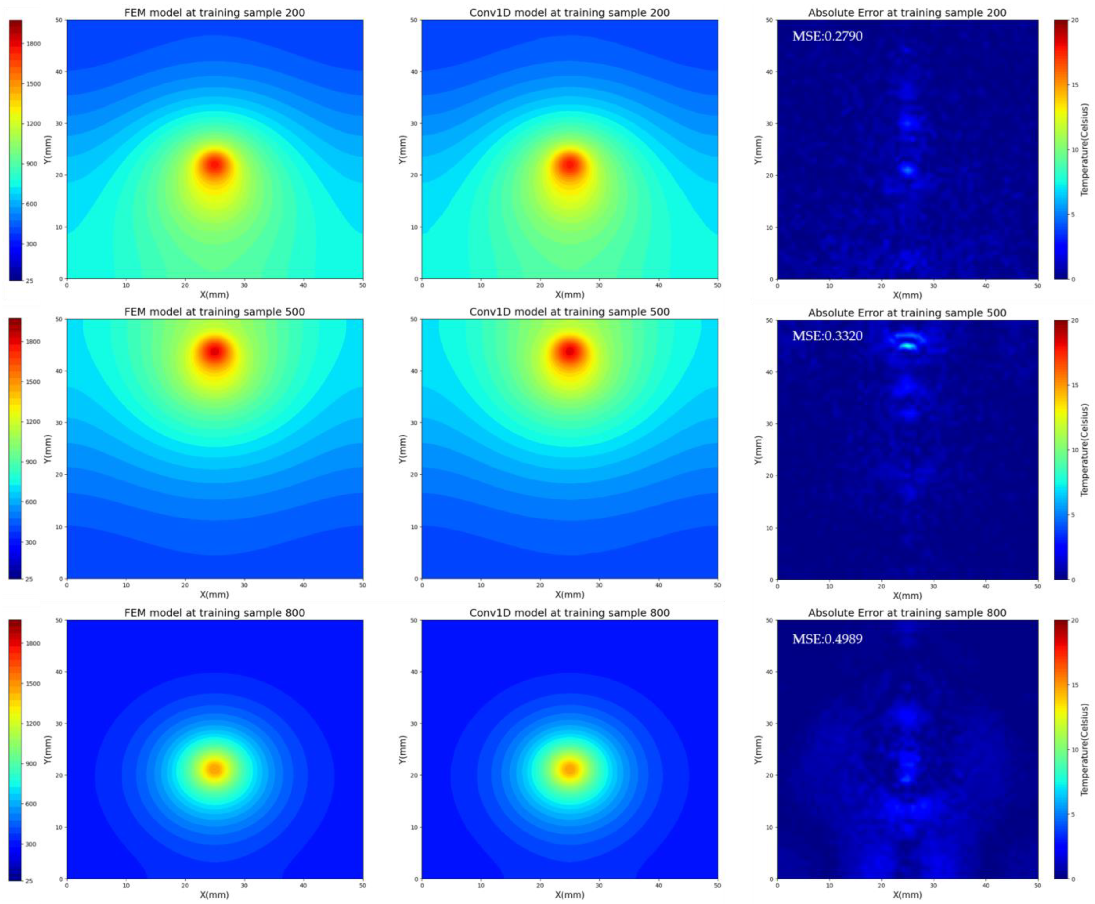
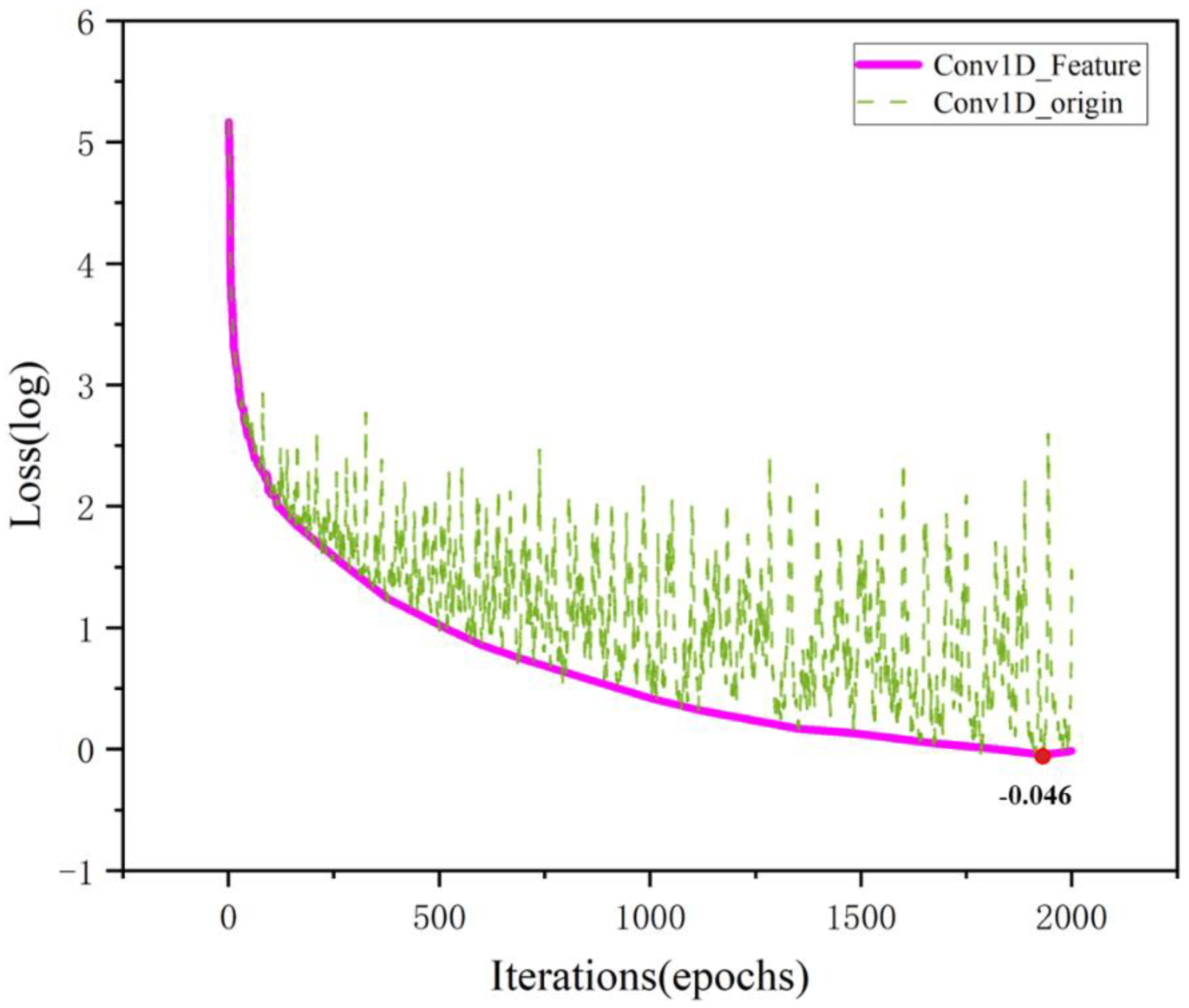
4.1. The Performance of Conv1D Model at Training Set

The loss value during the training process can intuitively reflect the prediction ability of the model. Figure 5 shows the changes in the loss value after taking the logarithm of the MSE loss function for 2000 iterations. When calculating the training loss, we restored the normalized output values so that they reflected the difference with the true temperature. The loss value reached an order of magnitude of 1 × 10⁵ at the beginning of the training stage, which means that the model failed to capture the characteristic relationship between the input and output. As the number of iterations increased, the training loss (log) gradually decreased to −0.046 in the gradient descent session. Since we set the learning rate to a fixed value, the gradient of the training loss may have been too large at each regression, which led to oscillations in the loss curve. In this experiment, the training loss of the model decreased with an increase in the training iterations, which means that the predicted results of the model became more accurate. To improve the training efficiency after the training loss decreased to 1 × 10³ and reduce the fluctuation amplitude so that the model could converge faster to the saddle point [38], it was necessary to reduce the value of the learning rate according to the training iterations [39].

After completing 2000 training iterations, the overall training loss of the Conv1D model was reduced to 0.8995 °C. Figure 6 lists the FEM temperature distribution (column 1), the predicted temperature distribution (column 2), and the absolute temperature error (column 3) at t = 4.5 s, t = 9 s, and t = 13.5 s, respectively. When the time step was 4.5 s, the peak temperature of the numerical simulation was 1707.4 °C and the predicted peak temperature was 1702.58 °C, with a minor difference of 4.82 °C. When deposition proceeded to the 9 s, the predicted result of the heat source moved in the same direction as the FEM result, and the error of the peak temperature was 4.35 °C. At 13.5 s, the peak temperature reached 1802.2 °C as deposition proceeded, at which point, the error of the peak temperature widened to 14.19 °C. We can see that the model’s temperature prediction was basically consistent with the actual situation, and the prediction accurately captured the heat conduction phenomenon in the process. In the given cases, the MSEs between the predicted temperature field and the temperature field calculated via numerical simulation were 1.5022 °C, 0.7936 °C, and 0.7803 °C, respectively. Three individual prediction cases show that the prediction performance of the Conv1D model reached a high level of accuracy in general. By comparing the absolute temperature error between the FEM and the Conv1D model, it can be observed that most of the prediction errors were concentrated in the molten pool region, where the temperature gradient changed fiercely. The training results show that the Conv1D model was able to accurately predict the characteristics of the temperature distribution, including the direction of heat source movement and the size of the melt pool, in the deposition process.

In the local temperature distribution, the neural network model still gave good results. Figure 7a shows the temperature distribution curves at the center of the path predicted by the Conv1D model and the numerical simulation at times t = 4.5 s, t = 9 s, and t = 13.5 s, respectively. The plot shows that the temperature values predicted by the neural network match well with the values calculated using the FEM, and the model’s predictions are numerically comparable to the true temperatures during the heating phase and the cooling phase. The relative error (RE) of the model is one of our focuses to evaluate the model’s prediction performance, and its expression is shown in Equation (10)

$$RE=\frac{\left|\widehat{T}\left(x,y\right)-T\left(x,y\right)\right|}{T\left(x,y\right)}\times 100\%$$

(10)

As shown in Figure 7b, in the region with a fierce temperature gradient, the model‘s prediction had large error fluctuations compared with the true temperature value. However, the prediction error was controlled within 20 °C, with a relative error is less than 1%. In the rest of the region, the prediction error could decrease to 5 °C or less, and its relative error was controlled within 0.5%. From the point of view of the prediction value’s accuracy, the prediction accuracy of the neural network model could reach more than 99%, and most of the errors were concentrated in the region of the huge temperature gradient. Moreover, considering the aspect of the limited influence that the maximum error value, which did not exceed 20 °C, brings to the actual manufacturing process, this is quite acceptable.

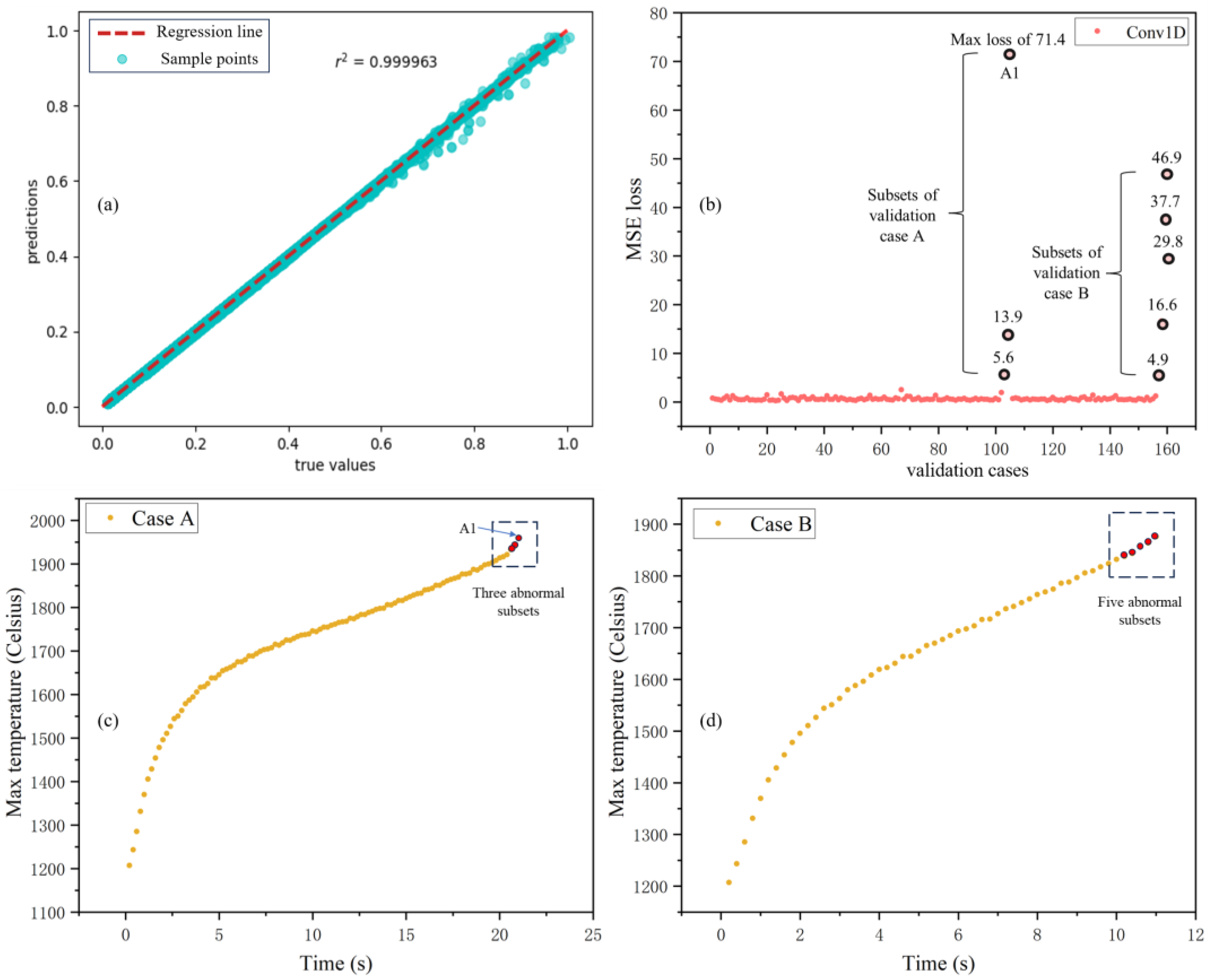
4.2. The Performance of Conv1D Model at Validation Set

The distribution of samples in the training set affected the training effect of the model. An unreasonable training set led to overfitting of the trained model, under which circumstances, the model’s error in the training set was small; still, the model’s performance in the validation set was poor. This means that the model had a poor understanding of the sample features and the robustness of the model was weak.

In order to evaluate the robustness of the Conv1D model, we built up a validation set consisting of two cases, A (Figure 8c) and B (Figure 8d). Each consisted of sub-steps with a time interval of 0.2 s, and the validation set contained a total of 161 samples. The coefficient of determination, R² (Equation (11)) and MSE loss, were used to measure the fitness of the Conv1D model to the validation set data.

$$R^2=1-\frac{{{\displaystyle \sum }}_1^N{\left[\widehat{T}\left(x,y\right)-T\left(x,y\right)\right]}^2}{{{\displaystyle \sum }}_1^N{\left[ T\left(x,y\right)-\overline{T}\left(x,y\right)\right]}^2}$$

(11)

In Figure 8a, we can see that the model had a good performance on the validation set. The individual sample data in the validation set, which are shown as the blue dots in the figure, fit the red regression line very well. The overall R2 value of the validation set was 0.999963, which is very close to the ideal value of 1. The overall MSE loss of the model was maintained around 0~5, as shown in Figure 8b. We note that there were a few samples with large error numbers in Cases A and B, with the biggest error of 71.38 occurring at Sample A1. Figure 8c,d indicate that these samples were located at the end of each deposition process, where the workpiece’s temperature continued to increase. Compared to those at the more stabilized manufacturing stage, the center of the heat source was close to the geometric boundary of the workpiece, and the shape of the high-temperature region changed due to the constraints of the geometric boundary of the workpiece. Therefore, new characteristics of the temperature distribution appeared. The new changes in the distribution characteristics of the temperature resulted in the precision of the model’s reconstructed temperature distribution not being accurate enough.

Figure 9 gives the absolute temperature errors for the A1 sample predicted by the model, with the true temperature and predicted temperature map listed on the bottom left. It can be seen from the figure that most of the prediction errors were concentrated in the high-temperature area, paralleled with the conclusion in Section 4.1. Furthermore, the model’s prediction of the position of the heat source center was quite accurate, while the prediction of the temperature distribution at the geometric boundary had a higher tolerance, where the maximum error exceeded the number of 110 °C and reached a relative error of 7.3%. This is consistent with the conclusion we made in the previous paragraph.

In order to improve the performance of the neural network model on the validation set, transfer learning is proposed to enhance the model’s prediction ability. The blue curve in Figure 10 shows the training loss (log) curve for the validation set; compared to the training loss in the base training, the value of the validation set’s initial loss was only 1 × 10². The training loss increased the first time due to the gradient value being too large in the first few iterations. Then, the value of the training loss continued to drop, as in the general case. After about 30 iterations, the loss dropped below 1, achieving the effect of 2000 iterations in the basic training. In addition, transfer learning works well with other datasets referring to new manufacturing parameters in the production process. Using transfer training methods tends to speed up the training procedure. The red curve in the figure shows the regression training with the trained Conv1D model’s parameters that match the temperature distribution dataset in the base training after changing the material properties. Compared to the basic training, the value of the new model’s training loss with transfer training was 100 times lower than that of base training. Reaching the same loss value of 1, the transfer training method shortened the training iterations by nearly 500 iterations, speeding up the model’s convergence velocity by 25%. Figure A1 and Figure A2 give additional prediction performances on the training set and the validation set.

The proposal of transfer training aimed to transform the model’s training process from a static state to a dynamic state. We can supplement the features of the training objects to fine-tune the model and improve the prediction robustness of the model. At the same time, we can use it to accelerate the training procedure to adapt the new object’s feature and save computational time.

4.3. The Performance of Conv1D Model for Computational Cost

A small computational cost while the machine learning model is running is preferred so that it can be deployed on adequate hardware. In addition, choosing the right model can satisfy the requirements on the response speed in the real manufacturing order. With accuracy requirements met, models with smaller computational costs and faster runtimes will have higher utility values.

Figure 11 compares the difference in the number of parameters between the Conv1D model and the commonly used fully connected neural network (FCNN) (40). In the convolutional stage, the number of parameters used in the Conv1D model was smaller than that of the FCNN model, floating from 10 times to 1000 times. It is noted that the definition of the machine learning model’s training parameters refers to those participating in forward and backward propagation, in which circumstance layers like max-pooling contain no training parameters. The advantage of the smaller number of parameters comes from the computation principle of the sliding convolution kernel on the input parameters shown in Figure 4 at Section 3, which makes the Conv1D model require significantly fewer parameters compared to the FCNN model when processing the same input data. Therefore, the Conv1D model has a significant advantage in terms of ROM occupation.

Figure 12a gives the training time required for both models over 200 to 2000 iterations and Figure 12b shows the highest accuracy achieved in the training stage. Although the Conv1D model has a more complex architecture than the FCNN model, the overall computation time was still quicker than that of the FCNN model due to the difference in the parameter numbers between the convolutional layer and the fully connected layer. As shown in Figure 12a, when the number of iterations reached 2000, the FCNN model took 26,245 s, while the Conv1D model took 20% less time, which was 21,042 s, to complete the training. Since the training parameters of the FCNN model were much greater than those of the Conv1D model, this resulted in the FCNN model having a slightly higher prediction accuracy than the Conv1D model in the overall training stage. However, when the number of iterations was increased to 1000 and above, the average prediction difference between the two models was less than 0.5 °C, which is numerically acceptable.

Table 4. Comparations between machine learning methods and finite element method.

	Running Time	Read-Only Memory Occupation	R2
Conv1D	0.7 s	52 MB	0.99999251
FCNN	1.2 s	111.5 MB	0.99999597
FEM	3 min 55 s	721 MB	1

gives the running time, Read-Only Memory occupation, and R2 performances of the three Conv1D, FCNN, and FEA models on the same dataset with a length of 100. In terms of running time, the two neural network models required much less time than the finite element model, with a time requirement of only 0.5% of the latter, while the Conv1D model took 0.5 s less time compared to the FCNN model, speeding up the forward propagation by about 50%. Considering the aspect of ROM occupation, the Conv1D model was only half the size of the FCNN model, occupying a size of 52 MB, and the size of the FEM results file was 14 times larger than that of the Conv1D model. As for accuracy, the difference between the three models was almost negligible.

Table 5. Comparison of the performance between the Conv1d model and typical ML models.

	Conv1d	Hua [39]	Spodniak [40]	Liao [41]	Xie [42]
MSE	0.8995	/	/	12.8881	18.6624
R2	0.9999	0.9995	0.9951	/	0.9980
Model type	1D-CNN	2D-CNN	FCNN	Physical-informed FCNN	Physical-informed FCNN

summarizes the performances of typical CNN and FCNN models. It can be seen that the overall accuracy of the CNN model was better than that of the FCNN model. With appropriate modification to the model structure, the prediction ability of the ML model can be improved. The three sections in this chapter provide a systematic evaluation corresponding to the dimensions of the Conv1D model’s accuracy, robustness, and capabilities. With the use of statistical methods such as MSE and R2, we can comprehend more clearly that the ML model has an excellent ability to derive the relationship between the process parameters and machining results in industrial manufacturing. At the same time, compared with the use of the FEM model, the ML model has a faster response ability and less operation consumption under the premise of ensuring the accuracy of the results. It provides a new approach for establishing fast accurate numerical simulation afterwards.

5. Conclusions

In this paper, a one-dimensional convolutional neural network was constructed for predicting the two-dimensional plane temperature distribution of a workpiece during plasma arc additive manufacturing processing using titanium–aluminum twin-wire. Through the reasonable use of machine learning, this paper explored a neural network combined numerical simulation method and process prediction workflow that included the finite element method, a convolutional neural network, and transfer learning. The accuracy of the prediction reached more than 99%. The main contributions of this paper can be summarized as follows:

• The article organically combined the FEM with the machine learning method and transfer training methods. A basic training and transfer training workflow was proposed, which provides a large amount of training data. At the same time, it transforms the model’s training process into a dynamic process to strengthen the model’s prediction robustness.
• The one-dimensional convolutional neural network model designed in this paper can effectively be fed one-dimensional processed features and predict temperature results during the manufacturing process. The MSE of the temperature field predicted by the neural network was reached within 0.5, and the prediction accuracy exceeded 99%.
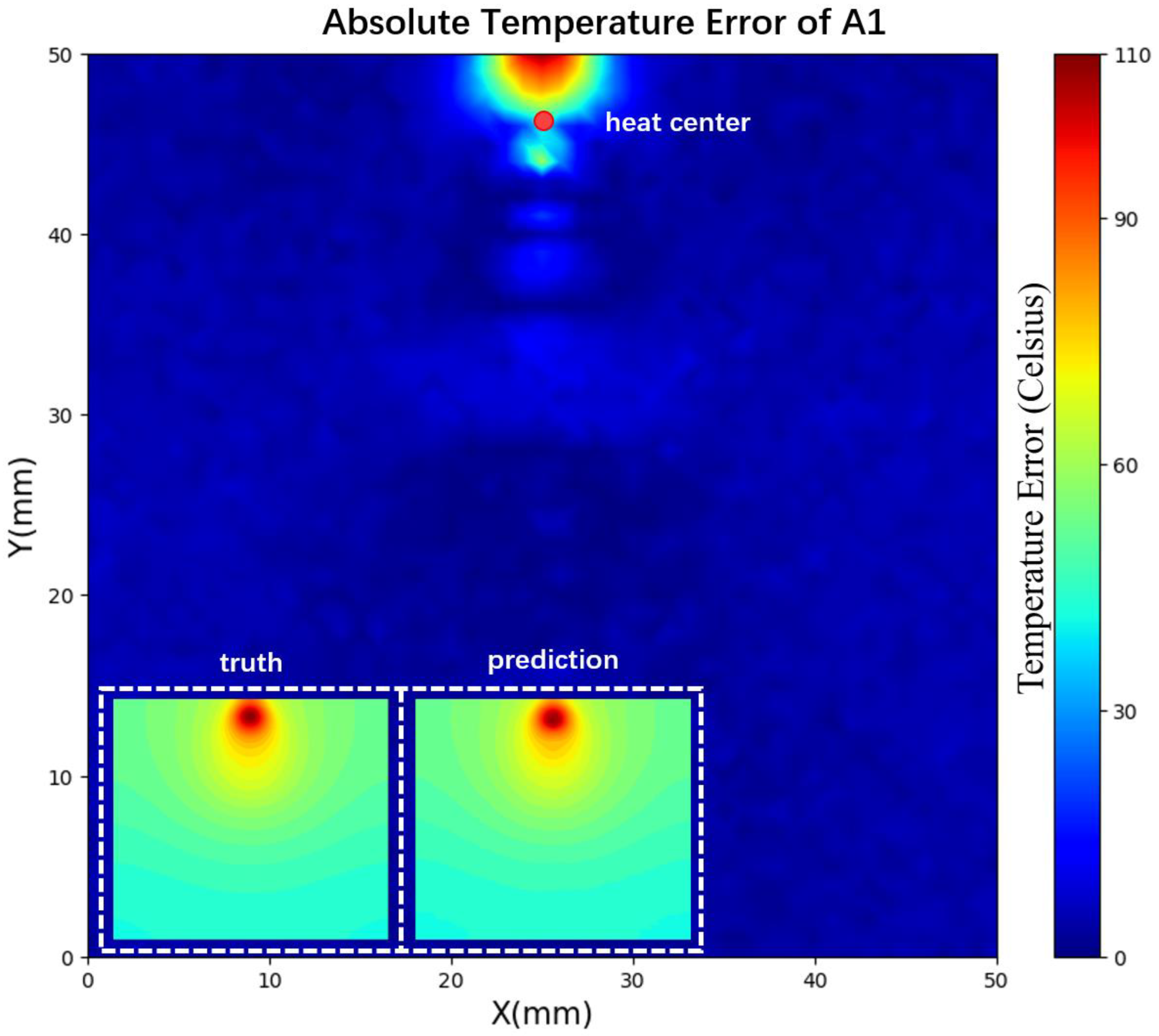
• The model performed well in the validation set and had a good robustness. The R² of the prediction results in the validation set could reach 0.999963, and the main error was concentrated in the high-temperature region of the workpiece. Through transfer training, the prediction error could be reduced to the desired value after 30 iterations.
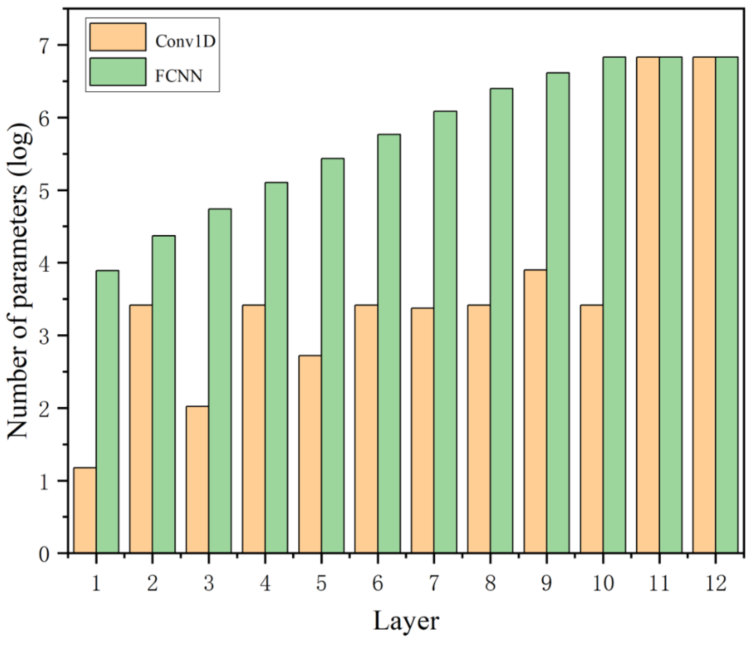
• The proposed Conv1D model had a better performance than the fully connected neural network model by using 50% of the running time, 80% of the training time, and only 50% of the ROM occupation. Compared with the traditional FEM prediction of temperature, the neural network model has obvious advantages in running time and ROM usage.

The characterization method of matching experimental parameters and experimental phenomena through neural networks will remain our focus in subsequent studies, and we will explore the relationship between other parameters and the prediction effect based on this study. In addition, there is still room for improvement in the structure of the ML model. We will continue to explore the construction of the model to obtain a more accurate, robust, and better-performing neural network model.

References

1. Zhou, W.L.; Jia, C.B.; Zhou, F.Z.; Wu, C.S. Dynamic evolution of keyhole and weld pool throughout the thickness during keyhole plasma arc welding. J. Mater. Process. Technol. 2023, 322, 118206. [Google Scholar] [CrossRef]
2. Zhu, Q.; Liu, Z.; Yan, J. Machine learning for metal additive manufacturing: Predicting temperature and melt pool fluid dynamics using physics-informed neural networks. Comput. Mech. 2021, 67, 619–635. [Google Scholar] [CrossRef]
3. Aghili, S.; Shamanian, M.; Najafabadi, R.A.; Keshavarzkermani, A.; Esmaeilizadeh, R.; Ali, U.; Marzbanrad, E.; Toyserkani, E. Microstructure and oxidation behavior of NiCr-chromium carbides coating prepared by powder-fed laser cladding on titanium aluminide substrate. Ceram. Int. 2020, 46, 1668–1679. [Google Scholar] [CrossRef]
4. Deng, L.; Hu, F.; Ma, M.; Huang, S.; Xiong, Y.; Chen, H.; Li, L.; Peng, S. Electronic Modulation Caused by Interfacial Ni-O-M (M = Ru, Ir, Pd) Bonding for Accelerating Hydrogen Evolution Kinetics. Angew. Chem. Int. Ed. 2021, 60, 22276–22282. [Google Scholar] [CrossRef] [PubMed]
5. Chen, X.L.; Liang, Z.L.; Guo, Y.H.; Sun, Z.G.; Wang, Y.Q.; Zhou, L. A study on the Grain Refinement Mechanism of Ti-6Al-4V Alloy Produced by Wire Arc Additive Manufacturing Using Hydrogenation Treatment Processes. J. Alloys Compd. 2021, 890, 161634. [Google Scholar] [CrossRef]
6. Chen, Y.; Lei, Z.L.; Heng, Z. Influence of laser beam oscillation on welding stability and molten pool dynamics. In Proceedings of the 24th National Laser Conference & Fifteenth National Conference on Laser Technology and Optoelectronics, Shanghai, China, 17–20 October 2020; Volume 11717, pp. 512–517. [Google Scholar] [CrossRef]
7. Fayazfar, H.; Salarian, M.; Rogalsky, A.; Sarker, D.; Russo, P.; Paserin, V.; Toyserkani, E. A critical review of powder-based additive manufacturing of ferrous alloys: Process parameters, microstructure and mechanical properties. Mater. Des. 2018, 144, 98–128. [Google Scholar] [CrossRef]
8. Liu, W.W.; Saleheen, K.M.; Tang, Z.J. Review on scanning pattern evaluation in laser-based additive manufacturing. Opt. Eng. 2021, 60, 070901. [Google Scholar] [CrossRef]
9. Jing, H.; Ye, X.; Hou, X.; Qian, X.; Zhang, P.; Yu, Z.; Wu, D.; Fu, K. Effect of Weld Pool Flow and Keyhole Formation on Weld Penetration in Laser-MIG Hybrid Welding within a Sensitive Laser Power Range. Appl. Sci. 2022, 12, 4100. [Google Scholar] [CrossRef]
10. Panwisawas, C.; Perumal, B.; Ward, R.W.; Turner, N.; Turner, R.P.; Brooks, J.W.; Basoalto, H.C. Keyhole formation and thermal fluid flow-induced porosity during laser fusion welding in titanium alloys: Experimental and modeling. Acta Mater. 2017, 126, 251–263. [Google Scholar] [CrossRef]
11. Trautmann, M.; Hertel, M.; Feussel, U. Numerical simulation of TIG weld pool dynamics using smoothed particle hydrodynamics. Int. J. Heat Mass Transf. 2017, 115, 842–853. [Google Scholar] [CrossRef]
12. Cho, W.I.; Woizeschke, P.; Schultz, V. Simulation of molten pool dynamics and stability analysis in laser buttonhole welding. Procedia CIRP 2018, 74, 687–690. [Google Scholar] [CrossRef]
13. Zhang, Y.J.; Hong, G.S.; Ye, D.S.; Zhu, K.P.; Fuh, J.Y.H. Extraction and evaluation of melt pool, plume and spatter information for powder-bed fusion AM process monitoring. Mater. Des. 2018, 156, 458–469. [Google Scholar] [CrossRef]
14. Shevchik, S.A.; Kenel, C.; Leinenbach, C.; Wasmer, K. Acoustic emission for in situ quality monitoring in additive manufacturing using spectral convolution neural networks. Addit. Manuf. 2018, 21, 598–604. [Google Scholar] [CrossRef]
15. Montazeri, M.; Rao, P. Sensor-Based Build Condition Monitoring in Laser Powder Bed Fusion Additive Manufacturing Process Using a Spectral Graph Theoretic Approach. J. Manuf. Sci. Eng. 2018, 140, 091002. [Google Scholar] [CrossRef]
16. Xie, X.; Bennett, J.; Saha, S.; Lu, Y.; Cao, J.; Liu, W.K.; Gan, Z. Mechanistic data-driven prediction of as-built mechanical properties in metal additive manufacturing. Comput. Mater. 2021, 7, 86. [Google Scholar] [CrossRef]
17. Chowdhury, S.; Anand, S. Artificial Neural Network Based Geometric Compensation for Thermal Deformation in Additive Manufacturing Processes. In Proceedings of the International Manufacturing Science and Engineering Conference, Blacksburg, VA, USA, 27 June–1 July 2016; Volume 3, p. V003T08A006. [Google Scholar] [CrossRef]
18. Mriganka, R.; Olga, W. Data-driven modeling of thermal history in additive manufacturing. Addit. Manuf. 2020, 32, 101017. [Google Scholar] [CrossRef]
19. Ren, K.; Chew, Y.; Zhang, Y.F.; Fuh, J.Y.H.; Bi, G.J. Thermal field prediction for laser scanning paths in laser aided additive manufacturing by physics-based machine learning. Comput. Methods Appl. Mech. Eng. 2020, 362, 112734. [Google Scholar] [CrossRef]
20. Raissi, M.; Perdikaris, P.; Karniadakis, G.E. Physics Informed Deep Learning (Part I): Data-driven Solutions of Nonlinear Partial Differential Equations. arXiv 2017, arXiv:1711.10561. [Google Scholar] [CrossRef]
21. Raissi, M.; Perdikaris, P.; Karniadakis, G.E. Physics Informed Deep Learning (Part II): Data-driven Solutions of Nonlinear Partial Differential Equations. arXiv 2017, arXiv:1711.10566. [Google Scholar] [CrossRef]
22. Baydin, A.G.; Pearlmutter, B.A.; Radul, A.A.; Siskind, J.M. Automatic differentiation in machine learning: A survey. J. Mach. Learn. Res. 2018, 18, 1–43. [Google Scholar] [CrossRef]
23. Lu, L.; Meng, X.H.; Mao, Z.P.; Karniadakis, G.E. DeepXDE: A Deep Learning Library for Solving Differential Equations. Soc. Ind. Appl. Math. 2021, 63, 208–228. [Google Scholar] [CrossRef]
24. Li, S.L.; Wang, G.; Di, Y.L.; Wang, L.P.; Wang, H.D.; Zhou, Q.J. A physics-informed neural network framework to predict 3D temperature field without labeled data in process of laser metal deposition. Eng. Appl. Artif. Intell. 2023, 120, 105908. [Google Scholar] [CrossRef]
25. Ren, K.; Chew, Y.; Liu, N.; Zhang, Y.F.; Fuh, J.Y.H.; Bi, G.J. Integrated numerical modeling and deep learning for multi-layer cube deposition planning in laser aided additive manufacturing. Virtual Phys. Prototyp. 2021, 16, 318–332. [Google Scholar] [CrossRef]
26. Zhu, Z.W.; Anwer, N.; Huang, Q.; Mathieu, L. Machine learning in tolerancing for additive manufacturing. CIRP Ann. 2018, 67, 157–160. [Google Scholar] [CrossRef]
27. Hemmasian, A.; Ogoke, F.; Akbari, P.; Malen, j.; Beuth, J.; Farimani, A.B. Surrogate modeling of melt pool temperature field using deep learning. Addit. Manuf. Lett. 2023, 5, 100123. [Google Scholar] [CrossRef]
28. Ness, K.L.; Paul, A.; Sun, L.; Zhang, Z.L. Towards a generic physics-based machine learning model for geometry invariant thermal history prediction in additive manufacturing. J. Mater. Process. Technol. 2022, 302, 117472. [Google Scholar] [CrossRef]
29. Zhang, S.W.; Kong, M.; Miao, H.; Memon, S.; Zhang, Y.J.; Liu, S.X. Transient temperature and stress fields on bonding small glass pieces to solder glass by laser welding: Numerical modeling and experimental validation. Sol. Energy 2020, 209, 350–362. [Google Scholar] [CrossRef]
30. Bai, X.; Colegrove, P.; Ding, J.; Zhou, X.; Diao, C.; Bridgeman, P.; Hönnige, J.R.; Zhang, H.; Williams, S. Numerical analysis of heat transfer and fluid flow in multilayer deposition of PAW-based wire and arc additive manufacturing. Int. J. Heat Mass Transf. 2018, 124, 504–516. [Google Scholar] [CrossRef]
31. Hou, X.; Ye, X.; Qian, X.; Zhang, X.; Zhang, P.; Lu, Q.; Yu, Z.; Shen, C.; Wang, L.; Hua, X. Heat Accumulation, Microstructure Evolution, and Stress Distribution of Ti–Al Alloy Manufactured by Twin-Wire Plasma Arc Additive. Adv. Eng. Mater. 2022, 1, 2101151. [Google Scholar] [CrossRef]
32. Hou, X.; Ye, X.; Qian, X.; Zhang, P.; Lu, Q.; Yu, Z.; Shen, C.; Wang, L.; Hua, X. Study on Crack Generation of Ti-Al Alloy Deposited by Plasma Arc Welding Arc. J. Mater. Eng. Perform. 2023, 32, 3574–3576. [Google Scholar] [CrossRef]
33. Li, C.; Zhang, S.H.; Qin, Y.; Estupinan, E. A systematic review of deep transfer learning for machinery fault diagnosis. Neurocomputing 2020, 407, 121–135. [Google Scholar] [CrossRef]
34. Hasan, M.J.; Kim, J.M. Bearing fault diagnosis under variable rotational speeds using stockwell transform-based vibration imaging and transfer learning. Appl. Sci. 2018, 8, 2357. [Google Scholar] [CrossRef]
35. Krizhevsky, A.; Sutskever, I.; Hinton, G.E. ImageNet classification with deep convolutional neural networks. Commun. ACM 2017, 60, 84–90. [Google Scholar] [CrossRef]
36. Badrinarayanan, V.; Kendall, A.; Cipolla, R. SegNet: A Deep Convolutional Encoder-Decoder Architecture for Image Segmentation. IEEE Trans. Pattern Anal. Mach. Intell. 2017, 39, 2481–2495. [Google Scholar] [CrossRef] [PubMed]
37. Rehmer, A.; Kroll, A. On the vanishing and exploding gradient problem in Gated Recurrent Units. IFAC-Pap. 2020, 53, 1243–1248. [Google Scholar] [CrossRef]
38. Esfamdiari, Y.; Balu, A.; Ebrahimi, K.; Vaidya, U.; Elia, N.; Sarkar, S. A fast saddle-point dynamical system approach to robust deep learning. Neural Netw. 2021, 139, 33–44. [Google Scholar] [CrossRef] [PubMed]
39. Hua, Y.; Yu, C.H.; Peng, J.Z.; Wu, W.T.; He, Y.; Zhou, Z.F. Thermal performance estimation of nanofluid-filled finned absorber tube using deep convolutional neural network. Appl. Sci. 2022, 12, 10883. [Google Scholar] [CrossRef]
40. Spodniak, M.; Semrád, K.; Draganová, K. Turbine Blade Temperature Field Prediction Using the Numerical Methods. Appl. Sci. 2021, 11, 2870. [Google Scholar] [CrossRef]
41. Liao, S.H.; Xue, T.J.; Jeong, J.; Webster, S.; Ehmann, K.; Cao, J. Hybrid thermal modeling of additive manufacturing processes using physics-informed neural networks for temperature prediction and parameter identification. Comput. Mech. 2023, 72, 499–512. [Google Scholar] [CrossRef]
42. Xie, J.B.; Chai, Z.; Xu, L.M.; Ren, X.K.; Liu, S.; Chen, X.Q. 3D temperature field prediction in direct energy deposition of metals using physics informed neural network. Int. J. Adv. Manuf. Technol. 2022, 119, 3449–3468. [Google Scholar] [CrossRef]
Figure 1. Schematic diagram of (a) the PAAW process; and (b) the thermal measure experiment.
Applsci 14 00661 g001
Figure 2. The general workflow of the dynamic training method. The * mark stands for changes in the datasets.
Applsci 14 00661 g002
Figure 3. The detailed structure of the proposed Conv1D network.
Applsci 14 00661 g003
Figure 4. Schematic diagram of operators in (a) convolution layer, (b) max pooling layer, and (c) linear layer.
Applsci 14 00661 g004
Figure 5. Loss curve of the Conv1D model in the training process.
Applsci 14 00661 g005
Figure 6. Two-dimensional temperature field and error distribution of Conv1D and FEM results in the deposition stage at t = 4.5 s, t = 9 s, and t = 13.5 s three substeps.
Applsci 14 00661 g006
Figure 7. Temperature distribution along the laser scanning track (y = 25 mm) at three different time steps in the deposition stage: (a) Absolute temperature and (b) temperature error.
Applsci 14 00661 g007
Figure 8. Scheme of (a) R2 values of validation sets, (b) MSE loss of validation sets, (c) temperature gradient rising at geometry boundary of case A, and (d) temperature gradient rising at geometry boundary of case B.
Applsci 14 00661 g008
Figure 9. Contour map of absolute temperature error at subset A1.
Applsci 14 00661 g009
Figure 10. Loss curves of transfer training and base training (300 epochs).
Applsci 14 00661 g010
Figure 11. Comparison of the parameter numbers between Conv1D model and FCNN model.
Applsci 14 00661 g011
Figure 12. Comparations between Conv1D model and FCNN model at perspectives of (a) training time and (b) accuracy.
Applsci 14 00661 g012