Abstract
In the context of scaling a business-critical medical service that involves electronic medical record storage deployed in Kubernetes clusters, this research addresses the need to optimize the configuration parameters of horizontal pod autoscalers for maintaining the required performance and system load constraints. The maximum entropy principle was used for calculating a load profile to satisfy workload constraints. By observing the fluctuations in the existing workload and applying a kernel estimator to smooth its trends, we propose a methodology for calculating the threshold parameter of a maximum number of pods managed by individual autoscalers. The results obtained indicate significant computing resource savings compared to autoscalers operating without predefined constraints. The proposed optimization method enables significant savings in computational resource utilization during peak loads in systems managed by Kubernetes. For the investigated case study, applying the calculated vector of maximum pod count parameter values for individual autoscalers resulted in about a 15% reduction in the number of instantiated nodes. The findings of this study provide valuable insights for efficiently scaling services while meeting performance demands, thus minimizing resource consumption when deploying to computing clouds. The results enhance our comprehension of resource optimization strategies within cloud-based microservice architectures, transcending the confines of specific domains or geographical locations.
1. Introduction
In recent years, the rapid evolution of cloud computing technologies has led to a significant shift in the deployment of large-scale information systems. Organizations are increasingly moving away from traditional on-premises data centers and embracing the advantages of cloud computing. Cloud platforms offer unparalleled benefits, including high availability, scalability, on-demand resource provisioning, and pay-as-you-go pricing models. These cloud-native features empower businesses to effortlessly configure services and only pay for the computational resources they consume, revolutionizing the way IT services are delivered [1].
As cloud adoption continues to grow, so does the need for efficient and dynamic resource allocation. Kubernetes, an open-source container orchestration platform, has emerged as a de facto standard for managing containerized workloads in cloud environments [2]. Kubernetes provides an automated and flexible approach to scaling services, with horizontal scaling, or the ability to multiply microservices deployed as containerized applications within pods, being paramount in cloud-native deployments.
The horizontal pod autoscaler (HPA) is a fundamental component of Kubernetes, enabling the automatic adjustment of microservice instances in response to changing system loads. The HPA allows for the dynamic scaling up or down of microservice instances based on predefined performance metrics [3]. Moreover, it offers an intriguing feature: the ability to provision new compute nodes when the current cluster configuration falls short of the required performance parameters. While this can greatly enhance system performance, it comes with associated costs.
The provisioning of new compute nodes introduces additional expenses, making it imperative to exercise control over this process, deploying new nodes only when justified. Standard HPA configuration parameters enable the definition of scaling conditions, such as setting a virtual CPU load threshold for a specific class of pods, above which new instances should be instantiated. However, HPAs tend to operate conservatively, maintaining a margin of available computational capacity. This conservative approach can lead to unnecessary provisioning of new compute nodes, especially when the upper limit of the system load is well-defined, which contributes to an increase in the total costs of ownership (TCO) indicator. Reducing the TCO should always be a priority when implementing and operating IT systems, as it enables enterprises to build a competitive advantage and contributes to sustainable resource management, particularly in terms of energy conservation. The TCO encompasses various dimensions, each influencing the overall operational cost of a system. Our specific focus lies within the infrastructural dimension, concentrating on the reduction of necessary computational resources. This reduction, achieved through the precise tuning of autoscaler parameters in Kubernetes environments, leads to a substantial decrease in the infrastructural component of the TCO. Effectively controlling computational resources is critical for organizations, enabling both significant financial savings and enhanced overall system performance. Thus, our study not only delves into the intricacies of infrastructural optimization but also delivers tangible benefits in the realm of IT cost management.
In this article, the authors propose a methodology to determine a maximum pod count limit. This methodology helps prevent the unnecessary provisioning of new compute nodes and optimizes the operational costs of the entire system. The proposed method was validated using a real-world example of a system deployed in Poland for storing medical patient records, where efficient resource utilization and cost-effectiveness are of paramount importance.
The paper makes significant contributions in the following areas:
- The development of a methodology for acquiring a load profile aligned with specified external conditions/restrictions, grounded in the maximum entropy principle (Section 4.1.1);
- Proposing a method of improving the load profile during peak times through kernel smoothing (Section 4.1.2);
- The formulation of an optimal configuration methodology, determining the optimal values for the maximum limits of pods utilized by horizontal pod autoscalers (Section 4.2); the method’s advantage lies in its proposal to reduce the dimensionality of the autoscaler parameter space (Section 4.2.3); the problem is streamlined from the multidimensional to one-dimensional by distributing limit values for all deployments proportionally (see Equation (10)) to a singular limit value for the highest-load deployment;
- The successful application of the proposed method to derive optimal upper limits for the autoscaler (Table 7) under real-world conditions and in the context of a real system (Clinical Data Repository).
However, the presented approach is not confined to the specific CDR system deployed in Poland. While the case study centers on the Polish medical system, the underlying principles and methodologies discussed herein are designed for broader application across diverse scenarios and geographic locations. Emphasizing cloud resource optimization through autoscaler parameter tuning in microservice architecture in Kubernetes deployments, our findings contribute to a comprehensive understanding of resource optimization strategies in cloud-based microservice architectures, transcending any specific industry or geographical constraints.
Following this introduction, the paper is structured into key sections to provide a comprehensive view of the research. The subsequent sections include Background and Related Work, which explains the context of the considerations presented in this paper and reviews the research related to the topic, Materials and Methods, where the research methodology is detailed, Results, where the findings are presented, and Conclusions, which summarize the significance of the research and its implications.
2. Background and Related Work
In today’s dynamic IT landscape, the deployment of applications in cloud computing environments has undergone a paradigm shift, moving away from traditional on-premises solutions towards the adoption of cloud-based platforms. This transition was driven by the desire for higher availability, scalability, and the removal of constraints on computational resources, all while enabling rapid provisioning of services and pay-as-you-go cost models. Amidst this evolution, Kubernetes has emerged as the de facto standard for container orchestration, automating the deployment and management of containerized applications within cloud clusters. It is worth noting that this shift has not only been observed by the scientific community but has also been actively fueled by researchers and practitioners, as evidenced by numerous publications on this topic. Interesting insights on the topic of deploying containerized systems to cloud environments are presented by Nikhil Marathe, Ankita Gandhi, and Jaimeel M Shah [4], where the authors addressed the challenges brought about by the increasing demand for cloud-based applications and the necessity for efficient resource utilization. This analysis encompasses a thorough exploration of container technologies, most notably Docker, and a meticulous investigation of orchestration tools such as Docker Swarm and Kubernetes. Through their research, the authors reveal the impact of these technologies on service availability within clusters, offering valuable insights through comparative analyses. The paper culminates with the presentation of research findings, which aim to enhance the performance of distributed computing systems in cloud contexts.
On the other hand, in other studies [5], researchers delve into the domain of virtualization technologies within high-performance computing (HPC) environments. Historically, the application of virtualization in HPC has been discouraged due to perceived performance overhead. However, with the emergence of container-based virtualization solutions such as Linux VServer, OpenVZ, and Linux Containers (LXC), a significant transformation has occurred, promising minimal overheads and performance nearly comparable to native setups. Within this research, the authors have conducted a meticulous series of experiments with the aim of providing an extensive performance evaluation of container-based virtualization in HPC. These results dispel any doubts regarding the effectiveness of container technology in the context of deploying applications in the cloud. However, while containerization has proved its worth in building efficient applications, its application alone is not a sufficient guarantee of achieving optimal resource utilization. Hence, the key focus shifts to building scalable applications, which can dynamically adjust the utilization of individual cloud computing resources to the current system load.
Kubernetes, as an orchestration platform for running microservices in computing clusters, implements various approaches to scale the applications. However, in the context of deployment in cloud computing environments, the most critical component is the horizontal pod autoscaler (HPA), which is responsible for monitoring the current workload and dynamically allocating computing resources, including provisioning new cluster nodes, to ensure the entire application can meet the current system load. It is, thus, clear to see why horizontal scaling and fine-tuning of HPA in Kubernetes clusters constitute hot topics in scientific research.
For example, the study titled “Leveraging Kubernetes for Adaptive and Cost-Efficient Resource Management” [6] aims to investigate how Kubernetes, a prevalent container orchestration framework, can enhance applications with adaptive performance management. The research emphasizes the utility of Kubernetes’ horizontal and vertical scaling concepts for adaptive resource allocation, along with an assessment of oversubscription as a method to simulate vertical scaling without application rescheduling. Through extensive experiments involving various applications and workloads, the study explores the impact of different scaling configurations on node resource utilization and application performance.
Autoscaling, an indispensable facet of cloud infrastructure, plays a crucial role in dynamically acquiring or provisioning computing resources to meet evolving demands. It enables automatic resource scaling for applications without human intervention, effectively optimizing resource costs while adhering to quality of service (QoS) requirements amidst fluctuating workloads. Kubernetes offers built-in autoscalers to address both vertical and horizontal scaling challenges at the container level. However, it exhibits certain limitations. The author of another study [7] conducted a comprehensive survey of existing approaches aimed at resolving container autoscaling challenges within the Kubernetes ecosystem. The survey encompasses an exploration of the primary characteristics of these approaches and highlights their ongoing issues. Drawing upon this analysis, the paper proposes potential future research directions to advance the field.
The authors of subsequent research [8] focus closely on the HPA component, which is also the subject of investigations within this study. Kubernetes monitors default resource metrics, encompassing CPU and memory usage on host machines and their pods. Additionally, custom metrics, provided by external software such as Prometheus, offer customization options to monitor a wide range of metrics. In their study, a series of experiments were conducted to investigate the HPA thoroughly and provide insights into its operational behavior. Furthermore, they discuss the significant differences between Kubernetes resource metrics (KRM) and Prometheus custom metrics (PCM) and their impact on HPA performance. The article concludes with valuable guidance and recommendations for optimizing HPA performance, serving as a valuable resource for researchers, developers, and system administrators involved in Kubernetes-related projects in the future.
A following paper [9] presents an innovative custom adaptive autoscaler called Libra. Libra’s primary function is to automatically identify the most suitable resource configuration for individual pods and oversee the horizontal scaling process. Furthermore, Libra exhibits the ability to dynamically adjust resource allocations for pods and adapt the horizontal scaling process to changing workloads or variations in the underlying virtualized environment.
Lastly, the researchers of another study [10] developed an autoscaler specifically designed for microservice applications in a Kubernetes environment. This autoscaler utilizes response time prediction as a core mechanism. The predictive model is created using machine learning techniques, which leverage performance metrics from both the microservice and node levels. The response time prediction aids in calculating the requisite number of pods necessary for the application to meet its predefined response time objectives. The experimental results indicate that the proposed autoscaler is capable of accommodating a higher volume of requests while maintaining the desired target response time compared to the Kubernetes horizontal pod autoscaler (HPA), which relies on CPU usage as its primary metric. However, it is worth noting that the proposed autoscaler consumes a higher amount of computational resources in achieving this performance improvement when compared to Kubernetes HPA.
Similar to the previously mentioned studies, the authors of this article also focus on performance, specifically aiming to maintain service response times at predefined levels as the system workload increases. However, the optimizations proposed in this case are carried out within the standard HPA component and involve its parameter tuning. The applied methods will be elaborated upon in the following section.
To verify the research directions, their progress, and their relevance in the ongoing scientific discourse, elements of a systematic literature review were used. For this purpose, the Scopus bibliographic database was used, which is considered one of the most suitable for this type of research [11]. In order not to miss relevant articles, all documents were retrieved according to the following query, which intentionally broadly defines the scope of the domain in question:
- TITLE-ABS-KEY ((k8s OR kubernetes) AND autoscaling AND (hpa OR autoscaler))
The query (as of 14 December 2023) retrieved 44 documents, of which, after verification, 15 were on topics consistent with those covered in this article (see Table 1). The oldest document was published in 2020, while 11 out of 15 articles were published between 2022 and 2023, which undoubtedly indicates that the issues discussed here are very topical.
It is noteworthy that all identified scientific works related to the addressed issues are centered around proposals for implementing autoscaler algorithms. These implementations predominantly leverage prediction methods based on complex neural networks such as GRU, RL, and LSTM. Alternatively, they focus on monitoring a set of parameters describing the current cluster operation and incorporating them into custom algorithms for calculating the desired number of pods in a given situation. The application of these methods is rather intricate and necessitates custom scaler implementations, raising concerns about their seamless integration into production environments. This would require extensive testing across various real-world production environments. In contrast, the proposed method in this article was built upon an existing and well-tested standard implementation of horizontal pod autoscaler (HPA), relying solely on the adjustment of one of its parameters. From this perspective, the approach is evidently innovative and, crucially, can be safely applied in production systems.

Table 1.
Scientific papers with converging topics.
Table 1.
Scientific papers with converging topics.
| Title | Year | Method Used |
|---|---|---|
| Toward Optimal Load Prediction and Customizable Autoscaling Scheme for Kubernetes [12] | 2023 | GRU |
| Intelligent Microservices Autoscaling Module Using Reinforcement Learning [13] | 2023 | RL |
| High Concurrency Response Strategy based on Kubernetes Horizontal Pod Autoscaler [14] | 2023 | custom formula |
| Proactive Horizontal Pod Autoscaling in Kubernetes Using Bi-LSTM [15] | 2023 | Bi–LSTM |
| Container Scaling Strategy Based on Reinforcement Learning [16] | 2023 | RL |
| Autoscaling Based on Response Time Prediction for Microservice Application in Kubernetes [10] | 2022 | ML |
| Traffic-Aware Horizontal Pod Autoscaler in Kubernetes-Based Edge Computing Infrastructure [17] | 2022 | custom formula |
| Horizontal Pod Autoscaling Based on Kubernetes with Fast Response and Slow Shrinkage [18] | 2022 | custom formula |
| K-AGRUED: A Container Autoscaling Technique for Cloud-based Web Applications in Kubernetes Using Attention-Based GRU Encoder-Decoder [19] | 2022 | GRU |
| LP-HPA:Load Predict-Horizontal Pod Autoscaler for Container Elastic Scaling [20] | 2022 | LSTM–GRU |
| DScaler: A Horizontal Autoscaler of Microservice Based on Deep Reinforcement Learning [21] | 2022 | RL |
| HANSEL: Adaptive Horizontal Scaling of Microservices Using Bi-LSTM [22] | 2021 | Bi–LSTM |
| Development of QoS-Aware Agents with Reinforcement Learning for Autoscaling of Microservices on The Cloud [23] | 2021 | RL |
| Deep Learning-Based Autoscaling Using Bidirectional Long Short-Term Memory for Kubernetes [24] | 2021 | Bi–LSTM |
| Adaptive Scaling of Kubernetes Pods [9] | 2020 | custom formula |
The demand for scaling systems to streamline the management of cloud computing resources has intensified, particularly for systems with broad applications and a large user base. It is not surprising that research on optimizing the scaling process of Kubernetes clusters is often conducted based on platforms supporting the healthcare sector [25,26,27]. In this domain, complex performance and security requirements pose unique challenges for system engineers [28].
3. Materials and Methods
3.1. Materials
In the concept of Kubernetes, containerization is a fundamental element, facilitating application isolation and portability. Containers encapsulate all necessary dependencies, addressing compatibility issues across various environments. Pods, the smallest manageable units in Kubernetes, group containers and share resources and network space.
Nodes constitute the cluster infrastructure where applications are executed. However, horizontal scaling is a pivotal feature of Kubernetes, enabling the dynamic adjustment of the number of application replicas in response to changing loads. Horizontal scaling involves adding or removing replicas (pods) based on the demand for computational resources. Mechanisms like the horizontal pod autoscaler (HPA) allow for the automatic adjustment of replica counts based on defined metrics, ensuring efficient resource management and optimal system performance. This approach enables dynamic infrastructure scaling (autoscaling) in response to variable workloads, which is crucial for effective and flexible application management in containerized environments.
The subject of the case study was a medical system developed for the gathering and archiving of clinical data (Clinical Data Repository—CDR), which serves as a medical data store for many hospital information systems (HIS) deployed according to a multitenant approach. The architecture of this system has been previously outlined in the context of earlier proprietary studies [29].
In this study, the focus is on controlling the number of pods to meet predefined constraints on the maximum service response time. However, the practical motivation for these considerations stems from the need to minimize the total cost of ownership (TCO) metric. Given the limited capacity of each node in the Kubernetes (K8s) cluster, an increase in the number of pods implies an increase in the number of nodes, resulting in higher costs. Therefore, reducing the number of pods limits the growth in resource consumption allocated by successive nodes in the Kubernetes cluster.
To monitor the load on individual pods, we employed two widely used technologies: Zipkin and Jaeger. Zipkin [30] is a distributed tracing system that helps gather timing data for operations in microservice architectures. It provides essential insights into the flow of requests among various components of a distributed system, aiding in the identification and resolution of performance bottlenecks. On the other hand, Jaeger [31] is an open-source, end-to-end distributed tracing system developed to monitor and troubleshoot transactions in complex, microservice-based architectures. It enables the visualization of the entire life cycle of requests, from initiation to completion, facilitating the analysis of system performance and identifying areas for improvement.
Additionally, for metrics collection, aggregation, and visualization, we employed the widely used toolset of Prometheus and Grafana. Prometheus [32] serves as a robust monitoring and alerting toolkit, while Grafana [33] complements it by offering a flexible and visually appealing platform for analyzing and presenting collected metrics.
To simulate the behavior of end-users and generate system load, we utilized the Gatling platform. Gatling [34] serves as a powerful tool for conducting performance tests and stress testing by simulating various user scenarios, providing insights into system behavior under different conditions.
To find the load profile according to data given by a client, some methods of mathematical modeling were used.
The data given by the client, describing an expected load, may be treated as some constraints for an unknown load profile. To find that load profile, we propose to use the maximum entropy principle [35,36,37]. The proposed method assumes that a normalized request load is considered as some unknown probability distribution. The maximum entropy principle assumes that the best probability distribution (describing the normalized load profile) subject to given constraints is the one which has the largest value of entropy. This allows for the conversion of the problem of obtaining the distribution describing the load profile into a problem of optimization with constraints. The MATLAB (fmincon) [38] was used to obtain values of probability and then minimize an optimization quality indicator based on the minus entropy of the distribution that we looked for.
To obtain the best possible approximation of the load (especially at peak), the proposed method assumes smoothing the angular distribution obtained after using the above-mentioned maximum entropy principle. The current distribution was used for obtaining the samples, which were used for calculating the new kernel-smoothed distribution [39,40,41]. The MATLAB platform (ksdensity) [42] was applied for smoothing.
3.2. Methods and Methodology
The primary objective was to acquire the optimal configuration for autoscaling mechanisms that ensure minimal consumption of computing resources during peak loads, adhering to predefined constraints for system efficiency and fault tolerance. The proposed methodology encompasses two integral components: the calculation of the load profile during peak periods and the empirical derivation of the optimal configuration for autoscalers tailored to the system’s load profile.
The first part pertains to identifying the appropriate test load profile. We presuppose the availability of initially provided values for the number of requests within specific time intervals throughout a day. These values are regarded as constraints that the unknown load profile must satisfy. The load profile, representing the most probable distribution of load intensity throughout a day, can be determined by minimizing the entropy of the unknown distribution while adhering to the specified constraints (that can be calculated using Algorithm 1 in Section 4.1.1).
We aimed to examine the system’s performance under peak load, focusing solely on the high segment of the acquired load profile. To isolate the peak load, the high-value portion of the load distribution is truncated and subjected to smoothing. Subsequently, the load distribution at peak, which is smoothed (by applying the so-called kernel smoothing algorithm, i.e., Algorithm 2 in Section 4.1.2) yet remains normalized to one, is scaled to meet the initially provided values for the number of requests across various time intervals throughout the day (Algorithm 3 in Section 4.1.3).
The second part of the proposed methodology pertains to the experimental derivation of upper limits for pod autoscalers, where pods represent fundamental computational units aggregated within deployments. The number of instantiated pods associated with a given deployment is regulated by an autoscaler. Given the system’s composition with multiple deployments (each having its autoscaler), exploring all conceivable settings (i.e., values of upper limits of pods for each deployment) leads to the overarching problem recognized as the curse of dimensionality. To circumvent this challenge, we advocate a phased approach wherein the relative dependencies among the numbers of pods in deployments are experimentally ascertained. Subsequently, the deployment with the highest number of instantiated pods is selected (Section 4.2.2). Proportionality ratios, relative to the selected deployment, are calculated for all deployments. This strategy enables adjustments solely to the setting of the chosen deployment and its corresponding autoscaler. The settings for the remaining autoscalers are interdependent, i.e., their values are proportional to those of the selected autoscaler (see Table 5). Consequently, this approach reduces the search space of autoscaler settings from multi- to one-dimensional space (Section 4.2.3).
Possessing an efficient one-dimensional method for adjusting autoscaler settings (see Table 6), we can experimentally validate them under the acquired peak load profile. The validation process involves assessing their compliance with certain constraints related to effectiveness and the correct operation (see Table 8), followed by selecting the settings that yield the lowest solution cost. Effectiveness can be evaluated through statistical measures of execution time, correctness by the ratio of improperly processed requests, and cost by the total number of instantiated pods, directly influencing the number of nodes (VMs) in a Kubernetes cluster.
4. Results
The way we obtained results for the system that is the subject of the case study, after applying the methods described in Section 3.2, is presented in the following subsections, which delve into the intricate details of the proposed method’s procedural steps and their application to the case study.
Section 4.1 presents the method of modeling the profile during load peaks that satisfies predefined performance requirements. Section 4.2 describes the approach to experimentally obtain cost-optimal parameters for autoscalers, enabling the entire system to meet the specified QoS requirements.
4.1. Obtaining the Peak Load Profile
This section describes and illustrates, through examples, the following processes:
- Determining a normalized load profile, characterized as a distribution that minimizes entropy while adhering to specified load requirements (Section 4.1.1);
- Extracting a segment of the load profile, specifically the load during peak periods, and subsequently smoothing its trajectory (Section 4.1.2);
- Scaling a normalized load during peak periods in accordance with predefined load requirements (Section 4.1.3).
4.1.1. Finding the Load Profile through the Maximum Entropy Principle
Let us assume the division of a day (24 h) into N equal intervals, where is the i-th interval, for .
Let be a normalized value of load in the i-th interval ().
All intervals overlap the 24 h: h.
Normalization means satisfying the following conditions: and .
The length of the i-th interval is .
The load given by a client is defined using subsections. Let us assume the following:
- —the m-th subsection;
- m—the number of subsections, where and ;
- —the number of requests in the m-th subsection ().
The domain of satisfies the following equations: h and
According to Equation (1):
- The beginning of the domain of is ;
- The end of the domain of is ;
- The length of the domain equals:
Let us assume that the subsection is the wider one, i.e., the subsection that has a domain that equals 24 h (a whole day). Then, for .
Let us define for as a normalized load “to the 1” in the subsection.
The sample of properties (the real examples) is presented in Table 2. A certain resolution of the interval division is also assumed, i.e., N = 48, so = 24 h/48 = 30 min.
Table 2.
Sample values of the load and time properties of subdivision located during a day.
Table 2.
Sample values of the load and time properties of subdivision located during a day.
| m | Beg-End of Sm Domain | [h] | [reqs] | [reqs/h] | |||
|---|---|---|---|---|---|---|---|
| 1 | 00:00–24:00 | 24 | 1 | 48 | 85,550 | 1 | 3564 |
| 2 | 11:00–17:00 | 6 | 22 | 33 | 56,780 | 0.66 | 9463 |
| 3 | 12:00–15:00 | 3 | 24 | 29 | 36,360 | 0.42 | 12,120 |
Let us present formulas defining the dependency between the and values for each m-th subsection:
According to the real data from Table 2 and using Equation (3), we can obtain concrete M = 3 equations:
This can be written in matrix expression:
where is presented in Table 3 and
- and .
Table 3.
Matrix A—the definition of the scope of subsections for .
Table 3.
Matrix A—the definition of the scope of subsections for .
| i | 1 | 2 | … | 21 | 22 | 23 | 24 | 25 | … | 29 | 30 | … | 33 | 34 | … | 48 |
|---|---|---|---|---|---|---|---|---|---|---|---|---|---|---|---|---|
| m | ||||||||||||||||
| 1 | 1 | 1 | … | 1 | 1 | 1 | 1 | 1 | … | 1 | 1 | … | 1 | 1 | … | 1 |
| 2 | 0 | 0 | … | 0 | 1 | 1 | 1 | 1 | … | 1 | 1 | … | 1 | 0 | … | 0 |
| 3 | 0 | 0 | … | 0 | 0 | 0 | 1 | 1 | … | 1 | 0 | … | 0 | 0 | … | 0 |
The next step in finding is based on the well-known maximum entropy principle. The crucial observation is that pairs can be treated as a discrete distribution with unknown values of probabilities .
The optimal vector of can be obtained by finding the maximum entropy. This is equivalent to the problem of finding the optimal (minimum) value of some quality indicator (minus entropy) subject to some constraints, i.e.,
where
The following is Algorithm 1 for finding normalized optimal values of returned in :
| Algorithm 1: Finding the optimal load profile using Entropy and load constrains. |
(input: A, R; output F_opt) 01 lb = [0,…, 0] // lower boundaries for f_i 02 ub = [1,…, 1] // upper boundaries for f_i 03 F_opt = fmin (minus_entropy, A, R, lb, ub) |
Function fmin can find the minimum of any multivariate function subject to some constraints. It accepts the following parameters:
Function minus_entropy is multivariate function that returns the opposite value of the function given by Equation (7).
A MATLAB-based program that implements Algorithm 1 and calculates for the considered real example is presented below:
- A = … % values are presented in Table 3
- R = [1, 0.66, 0.42]’
- lb = zeros(n,1); up = ones(n, 1) % lower and upper boundaries for f_i
- F_initial = rand(1, n) ./ n % initially, randomly around 1/n
- MinusEntropy = @(F) sum(F .* log2(F)) % defining of minus entropy function
- F_opt = fmincon(@MinusEntropy, F_initial, [], [], A, R, lb, ub)
- plot(F_opt)
The function fmincon [38] is a MATLAB implementation of the function fmin from Algorithm 1. The work-step results for obtaining the minimum with constraints using fmincon [38] are presented in Figure 1. Linear interpolation was applied.
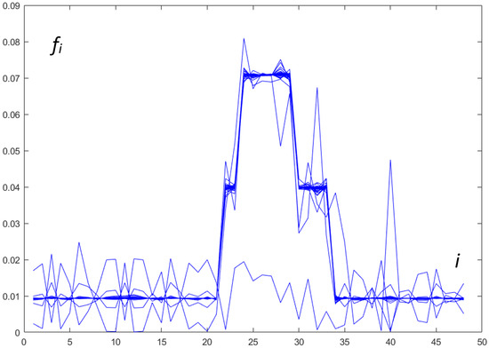
Figure 1.
Change of values of in each iteration of work steps of fmincon.
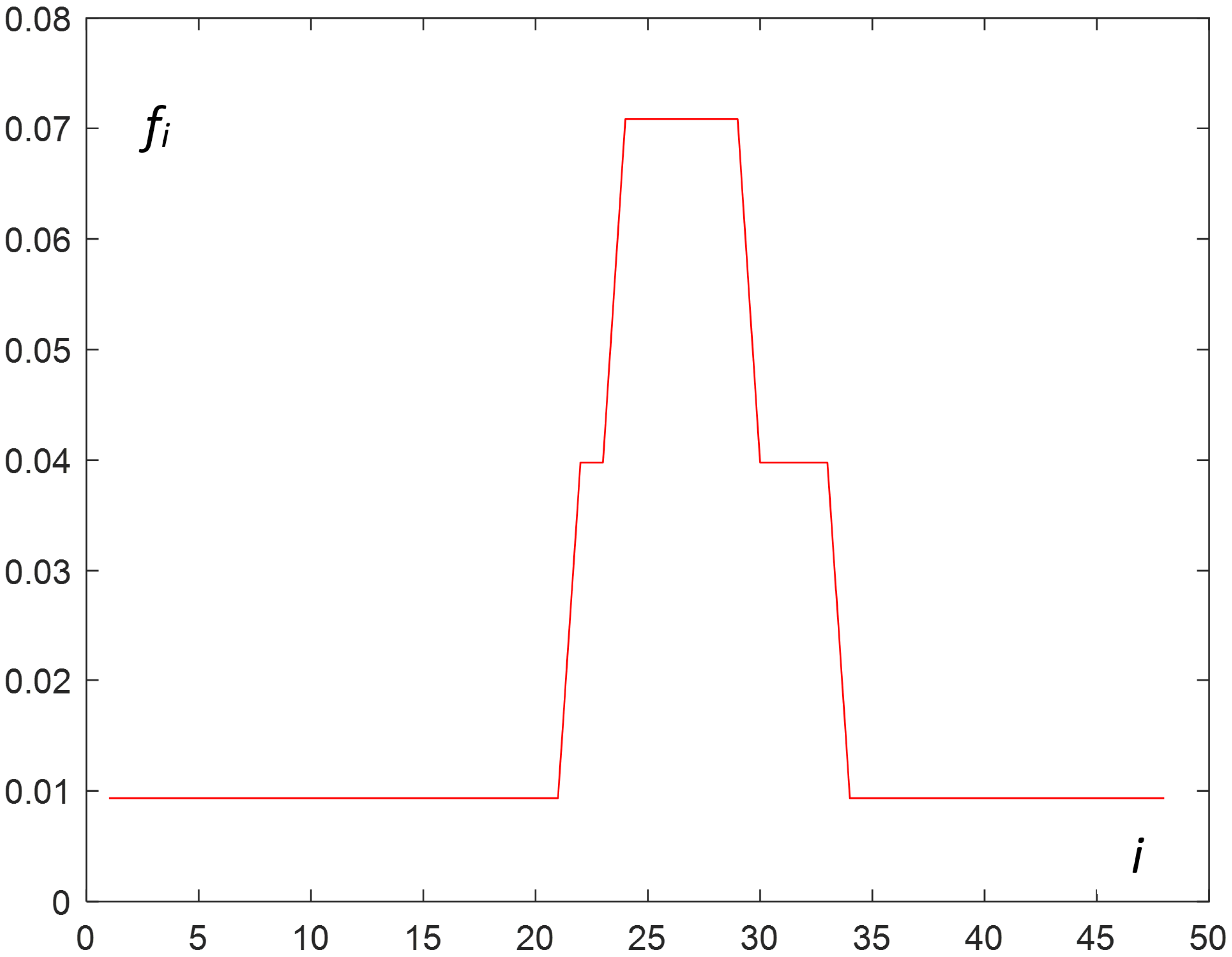
The values of found using Algorithm 1 are presented in Figure 2.
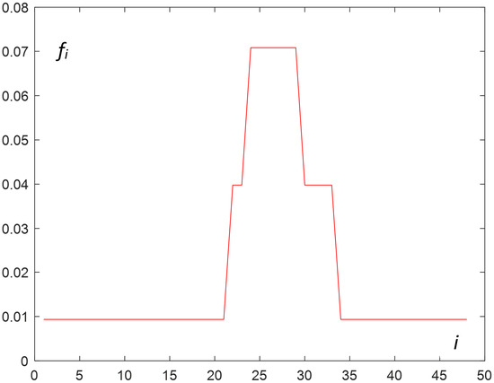
Figure 2.
Obtained optimal values of —the linear interpolation of normalized load.
4.1.2. Smoothing the Distribution of Load
Generally, broken curves (like the one in Figure 2) do not describe the real load, so the proposed method uses a selected smoothing technique. In the described method, the kernel smoothing for the distribution of the optimal (vector ) is proposed.
Algorithm 2, which was developed for calculating the smoothed distribution, is presented below:
| Algorithm 2: Calculating the smoothed load profile using kernel estimator. |
(input: F_opt; output: sF_opt) 01 // F_opt - vector of f_i for i = 1… n 02 // sF_opt - smoothed vector of f_i for i = 1… n 03 f_low = find the smallest value of f_i from F_opt 04 j = 1 05 sample = [] 06 for i = 1 to n 07 i_size = ceil (F_opt[i]/f_low) 08 // i_size-how many times index i should be represented in a sample 09 for k = 1 to i_size 10 sample [j++] = i 11 sF_opt = ks (sample, n) 12 // ks-generates a kernel-based density (n - values) using sample vector |
Algorithm 2 generates a sample containing indices, i.e., a set of i values of time intervals (see the beginning of Section 4.1.1). A value of the i index is repeated in the sample such (lines 07–10) that the interval is represented in the sample proportionally to the values from . Invoking the function ks (line 11) allows for the creation of an internal representation of the kernel-based density using the sample and then returns its values at points .
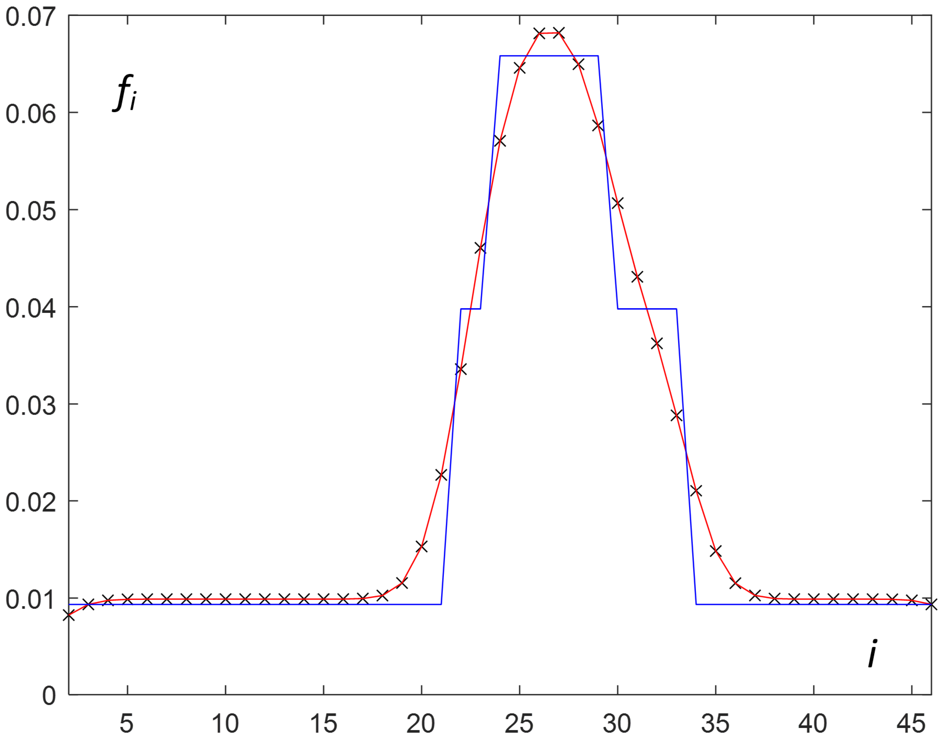
For the considered real example, the MATLAB function—ksdensity [42] with a Gaussian kernel—played the role of ks in Algorithm 2. The obtained smoothed distribution of (interpolated ) is presented in Figure 3.
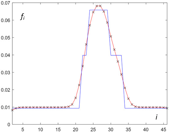
Figure 3.
Smoothed (red) and broken (blue) curves describing the continuous approximation of normalized load.
4.1.3. Obtaining the Approximate Load during a Peak
The last steps for obtaining the proper load profile refer to the calculation of the load during a peak. This could be obtained using the Algorithm 3 presented below:
| Algorithm 3: Obtaining adjusted load profile during a peak according to load restrictions. |
(input: sF_opt, subs_constr; output: peak_load ) 01 // sF_opt-normalized smoothed vector of f_i for a whole-day section 02 // subs_constr-description of subsection and load constrains-Table 2 03 // peak_load-he vector of load during subsection that load peak exists 04 m_peak = find m index where R_m/T_m has biggest value in subs_constr 05 // m_peak is an index of the most loaded subsection S_m_peak 06 R_m_peak = find value of absolute load for m_peak subsection in subst_constr 07 // calculate the sum of normalized loads in intervals belonging to the S_m_peak 08 sum = 0 09 for each (I_k in subsection S_m_peak) 10 sum = sum + sF_opt[k] 11 // calculate peak load by scaling R_m_peak 12 peak_load = [] 13 for each (I_k in subsection S_m_peak) 14 peak_load[k] = sF_opt[k]/sum * R_m_peak |
In line 04 of Algorithm 3, the subsection with the highest value of request per time from Table 2 is selected. Let us denote its index as .
Each value of the smoothed optimal normalized load that belongs to the -th subsection is scaled using the absolute load, i.e., .
Lines 08–14 are responsible for distributing the value according to the distribution, among the intervals included in the -th subsection, which can be expressed by Equation (8):
Such values are obtained (line 14) in values of the output vector .
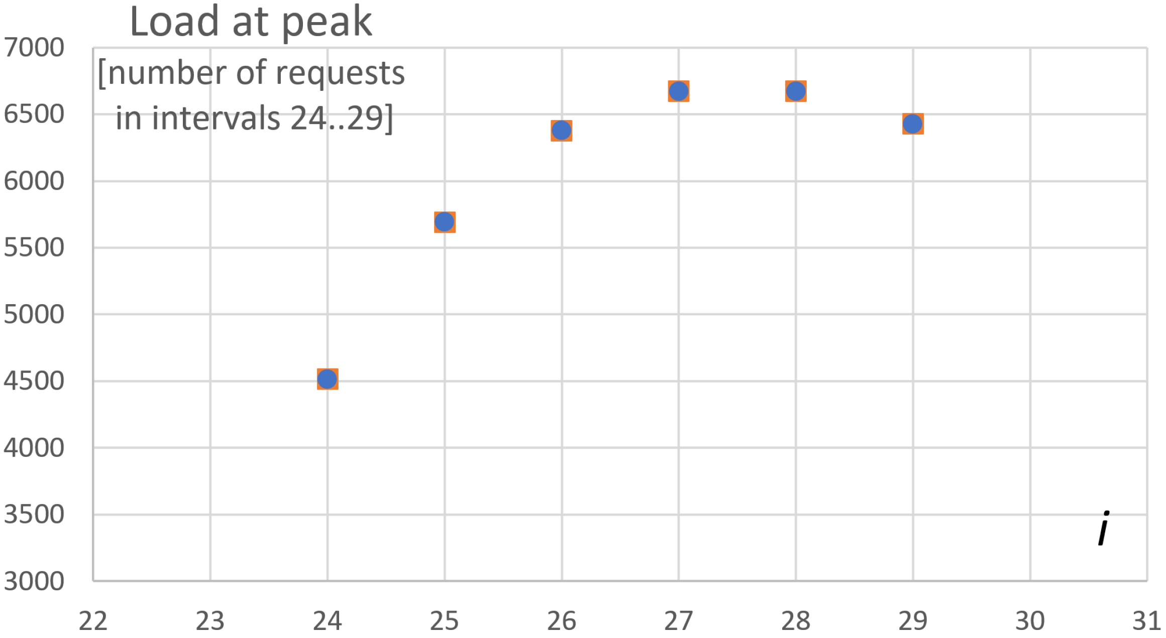
For the considered real example, according to the data from the column in Table 2, the highest load takes place for the 3rd subsection. This means that is 3, so the indices of intervals belonging to the peak are . The value of = 36,360 requests (Table 2) should be distributed among those intervals according to Equation (8). The resulting load at the peak for the assumed resolution (30 min intervals) is shown in Figure 4.
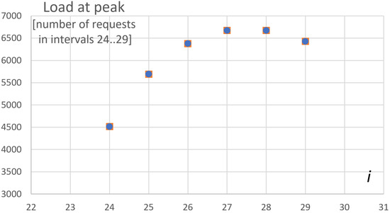
Figure 4.
The load during a peak (across 6 × 30 min = 3 h). The number of requests during each i-th interval for (each interval has a 30 min length).
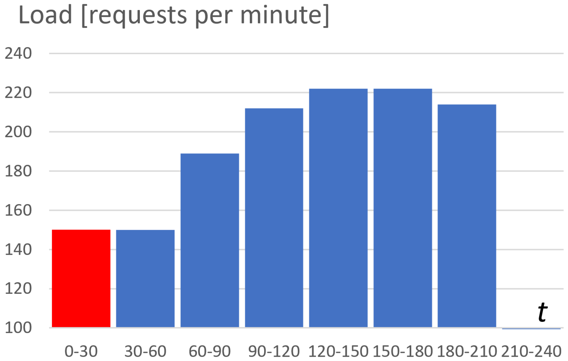
The resulting load profile is presented in Figure 5. The first part (the red bar) of the experiment for a time from 0 to 30 min is designated for the so-called warming of the system (to achieve a stable state of running pods). The exact peak (blue bars) is defined from 30 to 210 min. This part of the load profile is later used for gathering statistics data for obtaining the cost-efficiency characteristic of the considered system.

Figure 5.
Dependency between the result peak load profile (measured by requests per minute) and time.
4.2. Experimentally Obtaining the Upper Limits for Horizontal Autoscalers
This section describes the method for experimentally obtaining the values of the upper limits for horizontal autoscalers that fulfill the optimal number of running pods during a load peak. This section describes the following in detail (and presents examples):
- Experimentally detecting the pods (and deployments) involved in processing critical requests (Section 4.2.1);
- Experimentally obtaining the dependency between the numbers of pods of critical deployments (Section 4.2.2);
- Experimentally finding the optimal value of upper limits for autoscalers using the ratios from (3)—the crucial and final step in the method (Section 4.2.3).
4.2.1. Identifying Pods Involved in Handling Critical Requests
The system was tested against the flood of critical requests. In the context of the considered cloud-enabled Kubernetes-based CDR system [29], there were requests to create a medical document—a so-called ITI-41 transaction according to the IHE and PIK-HL7 standard.
The system consisted of many deployments that define several pods (about 200 for the considered system). Generally, for each deployment, at least two pods were instantiated. This results from satisfying a fault tolerance requirement. Some of pods should be instantiated in more than two pods for satisfying an efficiency condition given by a client. Of course, not all pods of the system were involved in handling the critical request.
As a result of the monitoring part of the system based on infrastructural components like Prometheus/Grafana (gathering statistics of processing by pod, nodes…) [32,34] and Jagger (tracing a particular request that passes microservices that run across pods) [31], it was possible to obtain complete lists of involved deployments. This is a list of critical deployments that define the pods involved in handling the critical request.
Let D denote the number of critical deployments. By observing the considered system experimentally, we obtained the value of .
4.2.2. Experimental Pod Multiplicity Dependency Analysis
The efficiency of the considered system is controlled by the HPA (horizontal pod autoscaler) [8]. The HPA is responsible for creating/destroying pods (belonging to a certain deployment) depending on a mean value of the CPU utilization of the pods. The mechanism of hysteresis is used for detecting the moments of instantiating additional pods (for too high a CPU utilization) or destroying pods (for too low a CPU utilization). Also, some constraints are taken into account by the HPA, i.e., the minimum number of pods—; and the maximum number of pods—.
was assumed in order to satisfy the fault tolerance assumption.
The role of is significant because of its impact on the number of pods during a very high load, which has a significant impact on the cost of the whole solution.
Each deployment has its own HPA (with own and ).
The problem lies in finding for each d where the system is sufficiently efficient, satisfies an error condition, and has a sufficiently low cost. This is rather a Pareto-optimal problem of finding the best values of the efficiency–cost complex quality indicator. This is also a D-dimensional problem and the solution must be found experimentally, which results in a high optimization task cost.
To overcome the problem of the so-called curse of dimensionality, we proposed disregarding all spaces of possible values of each . We propose to find an approximate dependency between the numbers of pods of critical deployments. This dependency can be obtained experimentally for some constant load whose value is based on a certain part of the given maximum load.
This dependency is later used in the proposed algorithm for changing the values of each . This allows the problem to be changed from a D-dimensional problem to the one-dimensional problem.
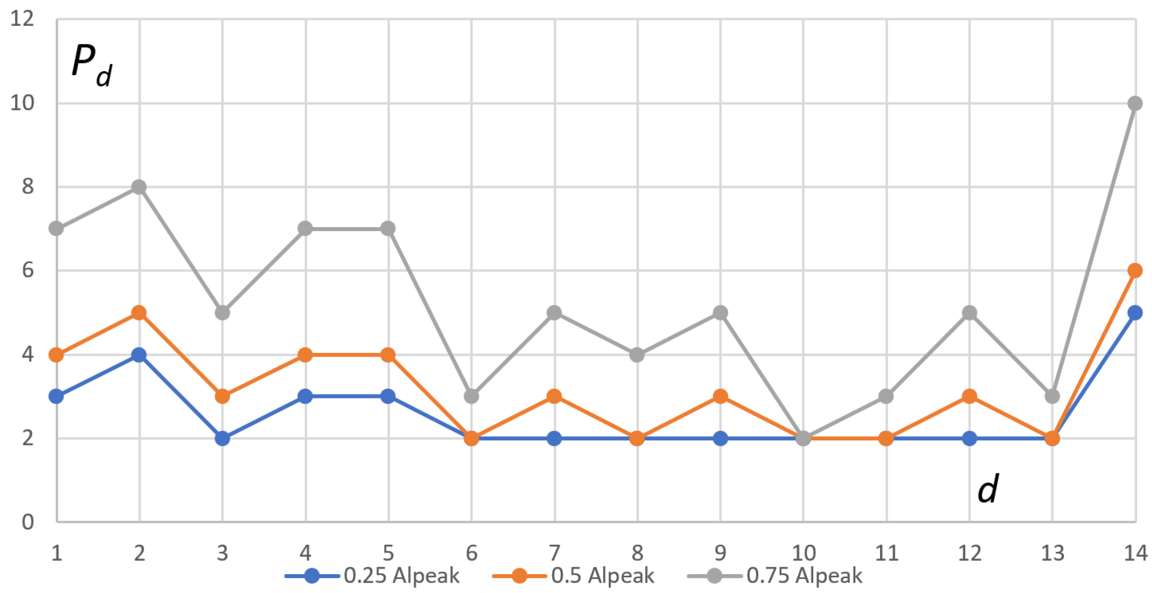
The characteristics the of number of instantiated pods () per critical deployment (d) obtained in experiments are shown in Table 4.
The restriction on the maximum number of pods was removed during of the subsequent three experiments. This allowed us to obtain the not-limited needs for pods that handle critical requests under the load for each the k-th experiment.
According to the values in Table 2 (the number of requests (36,360 requests) during the time of peak (3 h)), we calculated an average load at the maximum denoted as , which equals 202 requests per minute.
In the experiments, we used a constant load lasting 30 min. The value of the load for experiments was a fraction of , i.e., coefficients: 0.25, 0.5, and 0.75. Each k-th experiment was repeated (10 times) and the results were averaged and rounded to a natural value (see Table 4).
Table 4.
Values of the number of instantiated pods per deployment needed for handling the load in experiments.
Table 4.
Values of the number of instantiated pods per deployment needed for handling the load in experiments.
| k | 1 | 2 | 3 |
| 0.25 | 0.5 | 0.75 | |
| d | |||
| 1 | 3 | 4 | 7 |
| 2 | 4 | 5 | 8 |
| 3 | 2 | 3 | 5 |
| 4 | 3 | 4 | 7 |
| 5 | 3 | 4 | 7 |
| 6 | 2 | 2 | 3 |
| 7 | 2 | 3 | 5 |
| 8 | 2 | 2 | 4 |
| 9 | 2 | 3 | 5 |
| 10 | 2 | 2 | 2 |
| 11 | 2 | 2 | 3 |
| 12 | 2 | 3 | 5 |
| 13 | 2 | 2 | 3 |
| 14 | 5 | 6 | 10 |
Let us find the -th deployment with the greatest number of pods among all .
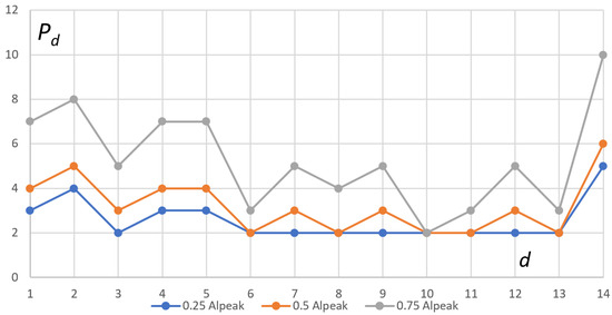
Figure 6.
Comparing the numbers of instantiated pods per deployment needed for handling the load in 3 experiments.
Let us use the result of the experiment to obtain the proportionality dependency between deployments.
Let us introduce the dependency coefficients normalized “to the one”, so:
- and . The deployment dependency for the considered example is shown in Table 5.
Table 5.
Coefficients of deployment dependency—relative numbers of required pods with respect to the most required deployment ().
Table 5.
Coefficients of deployment dependency—relative numbers of required pods with respect to the most required deployment ().
| d | 1 | 2 | 3 | 4 | 5 | 6 | 7 | 8 | 9 | 10 | 11 | 12 | 13 | 14 |
| 0.69 | 0.77 | 0.54 | 0.69 | 0.69 | 0.38 | 0.54 | 0.38 | 0.54 | 0.23 | 0.31 | 0.54 | 0.38 | 1.00 |
4.2.3. Finding the Optimal Setting of Parameter for HPAs
The last step in the proposed method allows the optimal values of to be established subject to the given constraints based on the median of times of request execution and %errors.
To find the optimal (or the Pareto-optimal) values of , we must consider changing and setting all D values for each experiment, which allows us to evaluate the assumed quality indicator. If we assume J different values for each , it will result in experiments.
Instead, we propose to only change the value of . is the value for the deployment that has the highest value of required pods, i.e., the deployment with the highest in Table 5. The rest of is calculated using the . This significantly decreases the number of required experiments.
Let us denote the following:
- J—the number of experiments;
- —the increase value (delta) of for the sequence of experiments;
- —the value of in the j-th experiment, where :
The values (in the j-th experiment) for other deployments are calculated proportionally to the coefficient from Table 5 (with respect to in the same j-th experiment):
In the considered example, we started the experiments from the value = 13. In addition, experiments were executed using the load profile described in Figure 5.
The values of where and are shown in Table 6.
Table 6.
The used values of for deployments in experiments.
Table 6.
The used values of for deployments in experiments.
| d | 1 | 2 | 3 | 4 | 5 | 6 | 7 | 8 | 9 | 10 | 11 | 12 | 13 | 14 |
|---|---|---|---|---|---|---|---|---|---|---|---|---|---|---|
| j | ||||||||||||||
| 1 | 9 | 10 | 7 | 9 | 9 | 5 | 7 | 5 | 7 | 3 | 4 | 7 | 5 | 13 |
| 2 | 10 | 11 | 8 | 10 | 10 | 5 | 8 | 5 | 8 | 3 | 4 | 8 | 5 | 15 |
| 3 | 11 | 13 | 9 | 11 | 11 | 6 | 9 | 6 | 9 | 3 | 5 | 9 | 6 | 17 |
| 4 | 13 | 14 | 10 | 13 | 13 | 7 | 10 | 7 | 10 | 4 | 5 | 10 | 7 | 19 |
| 5 | 14 | 16 | 11 | 14 | 14 | 8 | 11 | 8 | 11 | 4 | 6 | 11 | 8 | 21 |
| 6 | 15 | 17 | 12 | 15 | 15 | 8 | 12 | 8 | 12 | 5 | 7 | 12 | 8 | 23 |
| 7 | 17 | 19 | 13 | 17 | 17 | 9 | 13 | 9 | 13 | 5 | 7 | 13 | 9 | 25 |
| 8 | 18 | 20 | 14 | 18 | 18 | 10 | 14 | 10 | 14 | 6 | 8 | 14 | 10 | 27 |
| 9 | 20 | 22 | 15 | 20 | 20 | 11 | 15 | 11 | 15 | 6 | 8 | 15 | 11 | 29 |
Running the experiments on the considered system, according to HPA’s setting from Table 6 and the resulting load profile from Figure 5, allowed us to obtain the values of the mean numbers of pods per deployment, which are presented in Table 7.
Table 7.
Mean numbers of instantiated pods per deployment in 9 experiments under the limited HPAs using from Table 6.
Table 7.
Mean numbers of instantiated pods per deployment in 9 experiments under the limited HPAs using from Table 6.
| d | 1 | 2 | 3 | 4 | 5 | 6 | 7 | 8 | 9 | 10 | 11 | 12 | 13 | 14 | SUM |
|---|---|---|---|---|---|---|---|---|---|---|---|---|---|---|---|
| j | |||||||||||||||
| 1 | 8.9667 | 9.9596 | 6.9975 | 8.9049 | 8.9107 | 4.9132 | 6.9836 | 4.9935 | 6.9835 | 2.9617 | 3.9966 | 6.9657 | 4.9467 | 12.9871 | 99.47 |
| 2 | 9.8266 | 10.8679 | 7.9727 | 9.8781 | 9.8281 | 4.8318 | 7.9174 | 4.8102 | 7.8292 | 2.8903 | 3.8404 | 7.9783 | 4.9985 | 14.8373 | 108.31 |
| 3 | 10.8747 | 12.9698 | 8.6026 | 10.7859 | 10.9816 | 5.9280 | 8.8461 | 5.8075 | 8.8270 | 2.8627 | 4.8560 | 8.8575 | 5.9870 | 16.7610 | 122.95 |
| 4 | 12.8006 | 13.6271 | 9.4928 | 12.6719 | 12.7243 | 6.6601 | 9.4421 | 6.9883 | 9.5221 | 3.7223 | 4.9112 | 9.9391 | 6.5998 | 18.5931 | 137.69 |
| 5 | 13.4130 | 15.6568 | 10.7430 | 13.4009 | 13.6905 | 7.3995 | 10.3779 | 7.4713 | 10.6494 | 3.3574 | 5.9280 | 10.3957 | 7.5150 | 20.9460 | 150.94 |
| 6 | 14.8425 | 16.9452 | 11.3057 | 14.4380 | 14.9443 | 7.6105 | 11.2753 | 7.4316 | 11.6597 | 4.2873 | 6.3095 | 11.8167 | 7.6492 | 22.4450 | 162.96 |
| 7 | 16.4658 | 18.4884 | 12.9705 | 16.8384 | 16.4093 | 8.4676 | 12.3611 | 8.3710 | 12.6239 | 4.5416 | 6.5411 | 12.8192 | 8.6201 | 24.4102 | 179.93 |
| 8 | 17.0785 | 19.0732 | 13.8264 | 17.7213 | 17.8322 | 8.3784 | 13.9572 | 8.8037 | 13.0786 | 5.9261 | 6.5446 | 12.8818 | 8.5969 | 25.6859 | 189.38 |
| 9 | 19.9167 | 21.6530 | 13.2770 | 19.8088 | 19.1963 | 9.3961 | 13.3651 | 9.7983 | 13.4372 | 5.7085 | 6.0025 | 12.9293 | 8.9375 | 27.8380 | 201.26 |
The last column, named SUM, shows the total number of pods involved in handling the load in the j-th experiment. The number of pods had a direct impact on number of nodes provisioned by the Kubernetes cluster.
The final results according to the criteria of the evaluation are presented in Table 8.
The given efficiency indicator is based on the following:
- Me—the median of the execution times of the critical request;
- %error—the relative error (the number of failed requests compared to the total number of requests).
The given cost indicator is based on the number of compute components:
- NoN—the mean number of nodes of the Kubernetes cluster used by the considered system.
Generally, the best configuration could be selected as the optimal for a Pareto-optimal indicator based on Me, %error, and NoN. However, there are often known restrictions for some high-order quantile or the median of the execution times and %error. In the considered system, the client also gave the following conditions: Me < 2 ms and %error < 5%. Thus, we were only able to find acceptable configurations for . They are colored gray in Table 8.
Table 8.
The final results for the experiment: mean number of nodes (NoN), median request execution times (s) (Me), the relative error of responses (%).
Table 8.
The final results for the experiment: mean number of nodes (NoN), median request execution times (s) (Me), the relative error of responses (%).
| j | NoN | Me [s] | %error |
|---|---|---|---|
| 1 | 13.72 | 61.1 | 87.00% |
| 2 | 14.10 | 51 | 67.50% |
| 3 | 18.29 | 15 | 19.12% |
| 4 | 20.39 | 7.6 | 9.35% |
| 5 | 25.15 | 1.68 | 4.35% |
| 6 | 27.12 | 1.43 | 3.75% |
| 7 | 29.03 | 1.33 | 4.49% |
| 8 | 30.23 | 1.23 | 9.10% |
| 9 | 31.23 | 1.21 | 11.95% |
According to the obvious requirement of the lowest cost, we had to choose from 5, 6, and 7, because of the lowest NoN value, i.e., 25.15. Therefore, the cost-optimal setting of the value for HPAs handling critical pods has the index .
By analyzing the results of the specific experiments in Table 8, we managed to find a satisfactory solution that allowed us to save computational resources. If we compare the results for the acceptable solution—the most economical (NoN = 25.15 for j = 5)—and the fastest (Me = 1.33 s and NoN = 29.03 for j = 7), we obtain a savings coefficient (29.03 − 25.15)/25.15 × 100% .
The culmination of the research results is the resultant optimal vector of values of , which is highlighted in gray in Table 6.
5. Conclusions
In this study, we explored the critical aspects of scaling applications within Kubernetes clusters, specifically focusing on optimizing the configuration parameters of horizontal pod autoscalers (HPAs), to meet both performance and system load requirements efficiently. Through a rigorous examination of workload fluctuations and the application of kernel estimation techniques, we introduced a novel methodology for determining the maximum pod count limit, which is instrumental in minimizing resource provisioning costs.
This study has certain limitations that should be acknowledged. Firstly, this study aimed to develop a method for reducing the costs associated with the excessive utilization of computational resources during peak loads in mission-critical applications. The set goal was achieved, as confirmed by the experimental results. However, it is noteworthy that the greatest savings were achieved precisely during peak loads, while in other periods, the autoscaler operated according to its standard algorithm. Consequently, the most significant benefits from applying the proposed method will be observed in systems where low and moderate loads occur relatively infrequently within daily cycles. Secondly, the proposed method incorporates the assumption of knowing the volume of the maximum load. Therefore, it is clear that in exceptional situations involving its exceedance, the assumed performance criteria will no longer be met. Thirdly, the proposed method was illustrated using a system with a distinct daily load profile cycle, although its application is not limited solely to systems of such usage patterns. To apply it to systems with different load profile cycles, one would simply need to adjust the length of the adopted time window accordingly.
The results obtained from our research underscore the significant resource savings achieved by implementing our proposed methodology. By limiting the number of pods managed by individual HPAs, we effectively reduced the need for additional compute node provisioning. This not only led to cost reductions but also ensured the efficient allocation of resources in Kubernetes clusters.
The real-world application of our approach in the context of a CDR system in Poland demonstrated the practical benefits of our methodology. These findings emphasize the potential for improving the scalability and resource efficiency of cloud-native applications, especially when operating within the constraints of defined performance parameters.
The approach presented in this study is not limited to applications solely within the context of the specific CDR system deployed in Poland. While the specific case study focused on the Polish medical system, the underlying principles and methodologies discussed in the paper were designed to be applicable to a broader range of scenarios and geographic locations. The study’s emphasis on optimizing cloud computing resources through autoscaler parameter tuning in microservice architectures, particularly in Kubernetes deployments, provides generalizable insights that can be adapted and implemented in diverse contexts. The findings and recommendations put forth in this research contribute to the broader understanding of resource optimization strategies in cloud-based microservice architectures and are not confined to the healthcare domain or any specific geographical location.
In summary, our research contributes to the ongoing discourse on optimizing Kubernetes clusters for enhanced cost-effectiveness and resource utilization, with a specific focus on the pod count limit parameter. It is worth noting that our study concentrated on finding the parameter value that limits the number of instances of a given microservice class. However, another critical parameter, “cpu-percent”, which specifies the average CPU utilization over all pods, represented as a percentage of requested CPU, can also help preserve computing resources. Research on its impact and the selection of the optimal value may constitute a direction for further research.
Author Contributions
Conceptualization, D.R.A., Ł.W., and M.S.; methodology, D.R.A. and Ł.W.; software, D.R.A., Ł.W. and M.S.; validation, D.R.A. and Ł.W.; writing—original draft preparation, D.R.A. and Ł.W.; writing—review and editing, D.R.A. and Ł.W.; visualization, D.R.A. and M.S.; funding acquisition, D.R.A. and Ł.W. All authors have read and agreed to the published version of the manuscript.
Funding
This work was supported by Statutory Research funds of Department of Applied Informatics, Silesian University of Technology, Gliwice, Poland (02/100/BK_23/0027).
Institutional Review Board Statement
Not applicable.
Informed Consent Statement
Not applicable.
Data Availability Statement
The data presented in this study are available in article.
Conflicts of Interest
The authors declare no conflicts of interest.
Abbreviations
The following abbreviations are used in this manuscript:
| CDR | Clinical data repository |
| GRU | Gated recurrent unit |
| HIS | Hospital information system |
| HPA | Horizontal pod autoscaler |
| HPC | High performance computing |
| K8s | Kubernetes |
| KRM | Kubernetes resource metric |
| LSTM | Long short-term memory |
| LXC | Linux containers |
| ML | Machine learning |
| PCM | Prometheus custom metrics |
| QoS | Quality of service |
| RL | Reinforcement learning |
| TCO | Total cost of ownership |
References
- Armbrust, M.; Fox, A.; Griffith, R.; Joseph, A.D.; Katz, R.; Konwinski, A.; Lee, G.; Patterson, D.; Rabkin, A.; Stoica, I.; et al. A View of Cloud Computing. Commun. ACM 2010, 53, 50–58. [Google Scholar] [CrossRef]
- Burns, B.; Grant, B.; Oppenheimer, D.; Brewer, E.A.; Wilkes, J. Borg, Omega, and Kubernetes. Commun. ACM 2016, 59, 50–57. [Google Scholar] [CrossRef]
- Horizontal Pod Autoscaling. Available online: https://kubernetes.io/docs/tasks/run-application/horizontal-pod-autoscale/ (accessed on 6 November 2023).
- Marathe, N.; Gandhi, A.; Shah, J.M. Docker swarm and kubernetes in cloud computing environment. In Proceedings of the 2019 3rd International Conference on Trends in Electronics and Informatics (ICOEI), Tirunelveli, India, 23–25 April 2019; pp. 179–184. [Google Scholar]
- Xavier, M.G.; Neves, M.V.; Rossi, F.D.; Ferreto, T.C.; Lange, T.; De Rose, C.A. Performance evaluation of container-based virtualization for high performance computing environments. In Proceedings of the 2013 21st Euromicro International Conference on Parallel, Distributed, and Network-Based Processing, Belfast, UK, 27 February–1 March 2013; pp. 233–240. [Google Scholar]
- Verreydt, S.; Beni, E.H.; Truyen, E.; Lagaisse, B.; Joosen, W. Leveraging Kubernetes for Adaptive and Cost-Efficient Resource Management. In Proceedings of the WOC’19: 5th International Workshop on Container Technologies and Container Clouds, Davis, CA, USA, 9–13 December 2019; Association for Computing Machinery: New York, NY, USA, 2019; pp. 37–42. [Google Scholar] [CrossRef]
- Tran, M.N.; Vu, D.D.; Kim, Y. A Survey of Autoscaling in Kubernetes. In Proceedings of the 2022 Thirteenth International Conference on Ubiquitous and Future Networks (ICUFN), Barcelona, Spain, 5–8 July 2022; pp. 263–265. [Google Scholar] [CrossRef]
- Nguyen, T.T.; Yeom, Y.J.; Kim, T.; Park, D.H.; Kim, S. Horizontal Pod Autoscaling in Kubernetes for Elastic Container Orchestration. Sensors 2020, 20, 4621. [Google Scholar] [CrossRef] [PubMed]
- Balla, D.; Simon, C.; Maliosz, M. Adaptive scaling of Kubernetes pods. In Proceedings of the NOMS 2020—2020 IEEE/IFIP Network Operations and Management Symposium, Budapest, Hungary, 20–24 April 2020; pp. 1–5. [Google Scholar] [CrossRef]
- Pramesti, A.A.; Kistijantoro, A.I. Autoscaling Based on Response Time Prediction for Microservice Application in Kubernetes. In Proceedings of the 2022 9th International Conference on Advanced Informatics: Concepts, Theory and Applications (ICAICTA), Tokoname, Japan, 28–29 September 2022; pp. 1–6. [Google Scholar] [CrossRef]
- Ferreira Gregorio, V.; Pié, L.; Terceño, A. A Systematic Literature Review of Bio, Green and Circular Economy Trends in Publications in the Field of Economics and Business Management. Sustainability 2018, 10, 4232. [Google Scholar] [CrossRef]
- Mondal, S.K.; Wu, X.; Kabir, H.M.D.; Dai, H.N.; Ni, K.; Yuan, H.; Wang, T. Toward Optimal Load Prediction and Customizable Autoscaling Scheme for Kubernetes. Mathematics 2023, 11, 2675. [Google Scholar] [CrossRef]
- Abdel Khaleq, A.; Ra, I. Intelligent microservices autoscaling module using reinforcement learning. Clust. Comput. 2023, 26, 2789–2800. [Google Scholar] [CrossRef]
- Huo, Q.; Li, C.; Li, S.; Xie, Y.; Li, Z. High Concurrency Response Strategy based on Kubernetes Horizontal Pod Autoscaler. J. Phys. Conf. Ser. 2023, 2451, 012001. [Google Scholar] [CrossRef]
- Kakade, S.; Abbigeri, G.; Prabhu, O.; Dalwayi, A.; Narayan, G.; Patil, S.P.; Sunag, B. Proactive Horizontal Pod Autoscaling in Kubernetes using Bi-LSTM. In Proceedings of the IEEE International Conference on Contemporary Computing and Communications (InC4), Bangalore, India, 21–22 April 2023. [Google Scholar] [CrossRef]
- Wang, H.; Zhang, C.; Li, J.; Bao, D.; Xu, J. Container Scaling Strategy Based on Reinforcement Learning. Secur. Commun. Netw. 2023, 2023, 7400235. [Google Scholar] [CrossRef]
- Phuc, L.H.; Phan, L.A.; Kim, T. Traffic-Aware Horizontal Pod Autoscaler in Kubernetes-Based Edge Computing Infrastructure. IEEE Access 2022, 10, 18966–18977. [Google Scholar] [CrossRef]
- Huo, Q.; Li, S.; Xie, Y.; Li, Z. Horizontal Pod Autoscaling based on Kubernetes with Fast Response and Slow Shrinkage. In Proceedings of the 2022 International Conference on Artificial Intelligence, Information Processing and Cloud Computing (AIIPCC), Kunming, China, 19–21 August 2022; pp. 203–206. [Google Scholar] [CrossRef]
- Dogani, J.; Khunjush, F.; Seydali, M. K-AGRUED: A Container Autoscaling Technique for Cloud-based Web Applications in Kubernetes Using Attention-based GRU Encoder-Decoder. J. Grid Comput. 2022, 20, 40. [Google Scholar] [CrossRef]
- Xu, Y.; Qiao, K.; Wang, C.; Zhu, L. LP-HPA:Load Predict-Horizontal Pod Autoscaler for Container Elastic Scaling. In Proceedings of the CSSE ’22: Proceedings of the 5th International Conference on Computer Science and Software Engineering, Guilin, China, 21–23 October 2022; pp. 591–595. [Google Scholar] [CrossRef]
- Xiao, Z.; Hu, S. DScaler: A Horizontal Autoscaler of Microservice Based on Deep Reinforcement Learning. In Proceedings of the 2022 23rd Asia-Pacific Network Operations and Management Symposium (APNOMS), Takamatsu, Japan, 28–30 September 2022. [Google Scholar] [CrossRef]
- Yan, M.; Liang, X.; Lu, Z.; Wu, J.; Zhang, W. HANSEL: Adaptive horizontal scaling of microservices using Bi-LSTM. Appl. Soft Comput. 2021, 105, 107216. [Google Scholar] [CrossRef]
- Khaleq, A.A.; Ra, I. Development of QoS-aware agents with reinforcement learning for autoscaling of microservices on the cloud. In Proceedings of the 2021 IEEE International Conference on Autonomic Computing and Self-Organizing Systems Companion (ACSOS-C), Washington, DC, USA, 27 September–1 October 2021; pp. 13–19. [Google Scholar] [CrossRef]
- Dang-Quang, N.M.; Yoo, M. Deep learning-based autoscaling using bidirectional long short-term memory for kubernetes. Appl. Sci. 2021, 11, 3835. [Google Scholar] [CrossRef]
- Baptista, T.; Silva, L.B.; Costa, C. Highly scalable medical imaging repository based on Kubernetes. In Proceedings of the 2021 IEEE International Conference on Bioinformatics and Biomedicine (BIBM), Houston, TX, USA, 9–12 December 2021; pp. 3193–3200. [Google Scholar]
- Augustyn, D.R.; Wyciślik, Ł.; Sojka, M. The FaaS-Based Cloud Agnostic Architecture of Medical Services—Polish Case Study. Appl. Sci. 2022, 12, 7954. [Google Scholar] [CrossRef]
- Masouros, D.; Koliogeorgi, K.; Zervakis, G.; Kosvyra, A.; Chytas, A.; Xydis, S.; Chouvarda, I.; Soudris, D. Co-design implications of cost-effective on-demand acceleration for cloud healthcare analytics: The AEGLE approach. In Proceedings of the 2019 Design, Automation & Test in Europe Conference & Exhibition (DATE), Florence, Italy, 25–29 March 2019; pp. 622–625. [Google Scholar]
- Aceto, G.; Persico, V.; Pescapé, A. Industry 4.0 and health: Internet of things, big data, and cloud computing for healthcare 4.0. J. Ind. Inf. Integr. 2020, 18, 100129. [Google Scholar] [CrossRef]
- Augustyn, D.R.; Wyciślik, Ł.; Sojka, M. The Cloud-Enabled Architecture of the Clinical Data Repository in Poland. Sustainability 2021, 13, 14050. [Google Scholar] [CrossRef]
- Zipkin. Available online: https://zipkin.io/ (accessed on 6 November 2023).
- Jaeger. Available online: https://www.jaegertracing.io/ (accessed on 6 November 2023).
- Prometheus. Available online: https://prometheus.io/ (accessed on 6 November 2023).
- Grafana. Available online: https://grafana.com/ (accessed on 6 November 2023).
- Gatling. Available online: https://gatling.io/ (accessed on 6 November 2023).
- Guiasu, S.; Shenitzer, A. The principle of maximum entropy. Math. Intell. 1985, 7, 42–48. [Google Scholar] [CrossRef]
- Cesari, A.; Reißer, S.; Bussi, G. Using the maximum entropy principle to combine simulations and solution experiments. Computation 2018, 6, 15. [Google Scholar] [CrossRef]
- Jaynes, E.T. On the rationale of maximum-entropy methods. Proc. IEEE 1982, 70, 939–952. [Google Scholar] [CrossRef]
- Find Minimum of Constrained Nonlinear Multivariable Function. Available online: https://uk.mathworks.com/help/optim/ug/fmincon.html (accessed on 6 November 2023).
- Chung, M.K. Gaussian kernel smoothing. arXiv 2020, arXiv:2007.09539. [Google Scholar]
- Peter D, H. Kernel estimation of a distribution function. Commun. Stat.Theory Methods 1985, 14, 605–620. [Google Scholar] [CrossRef]
- Ghosh, S. Kernel Smoothing: Principles, Methods and Applications; John Wiley & Sons: Hoboken, NJ, USA, 2018. [Google Scholar]
- Kernel Smoothing Function Estimate for Univariate and Bivariate Data. Available online: https://uk.mathworks.com/help/stats/ksdensity.html/ (accessed on 6 November 2023).

Disclaimer/Publisher’s Note: The statements, opinions and data contained in all publications are solely those of the individual author(s) and contributor(s) and not of MDPI and/or the editor(s). MDPI and/or the editor(s) disclaim responsibility for any injury to people or property resulting from any ideas, methods, instructions or products referred to in the content. |
© 2024 by the authors. Licensee MDPI, Basel, Switzerland. This article is an open access article distributed under the terms and conditions of the Creative Commons Attribution (CC BY) license (https://creativecommons.org/licenses/by/4.0/).