Author Contributions
Conceptualization, N.Z. and S.Y.; methodology, S.Y.; software, J.W.; validation, S.Y., H.W. and X.Z.; formal analysis, N.Z.; investigation, J.W.; resources, T.L.; data curation, H.W.; writing—original draft preparation, S.Y.; writing—review and editing, S.Y.; visualization, N.Z.; supervision, J.W.; project administration, T.L.; funding acquisition, X.Z. All authors have read and agreed to the published version of the manuscript.
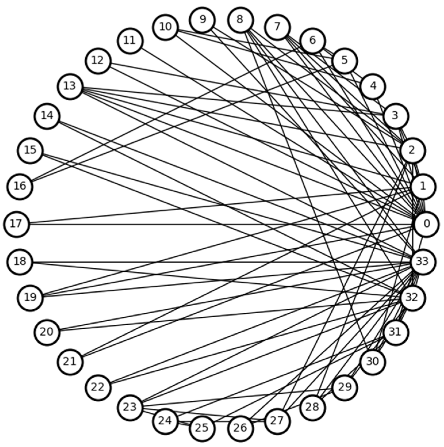
Figure 1.
Karate network. The numbers in the figure indicate the node numbers.
Figure 1.
Karate network. The numbers in the figure indicate the node numbers.
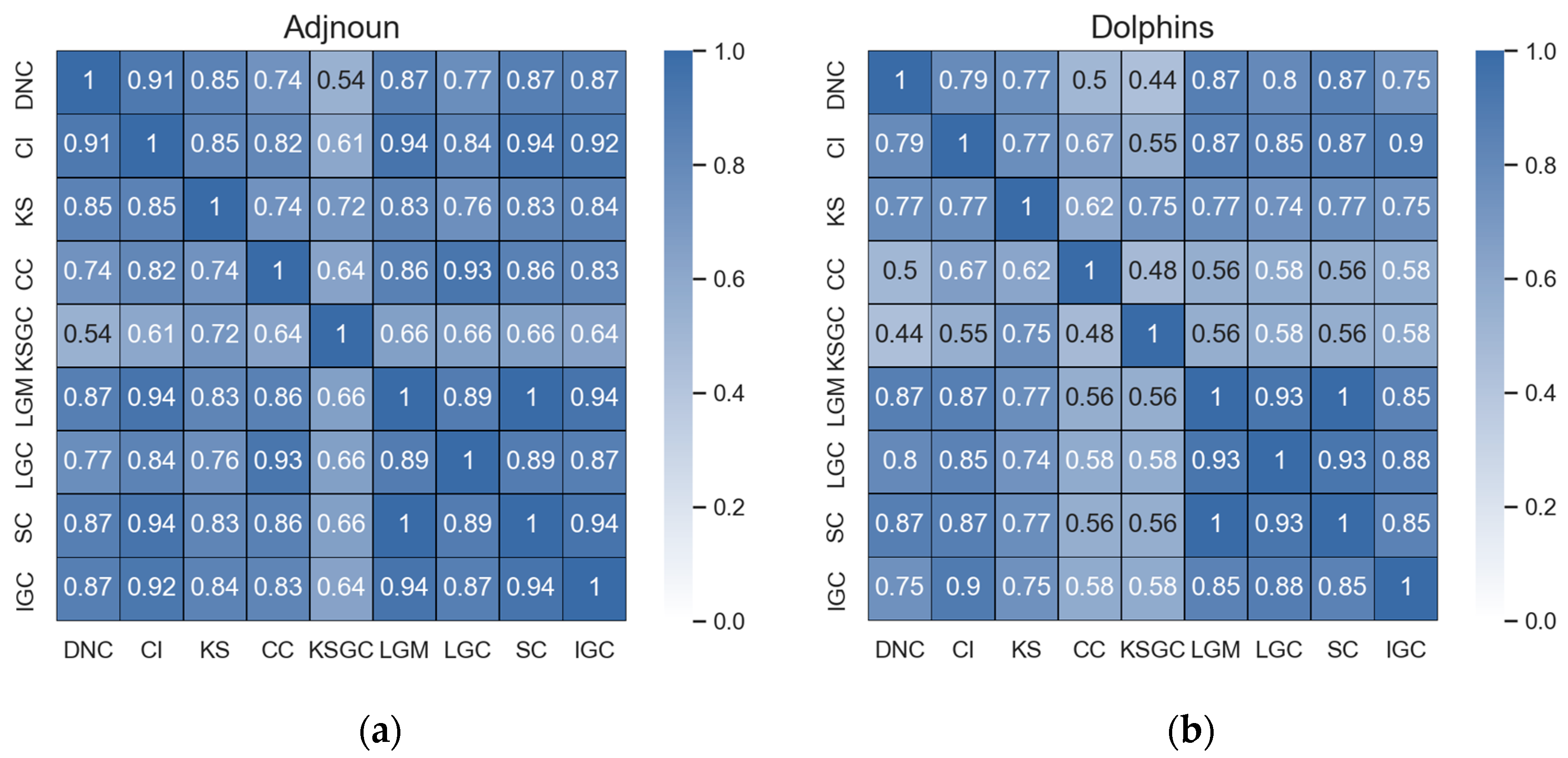
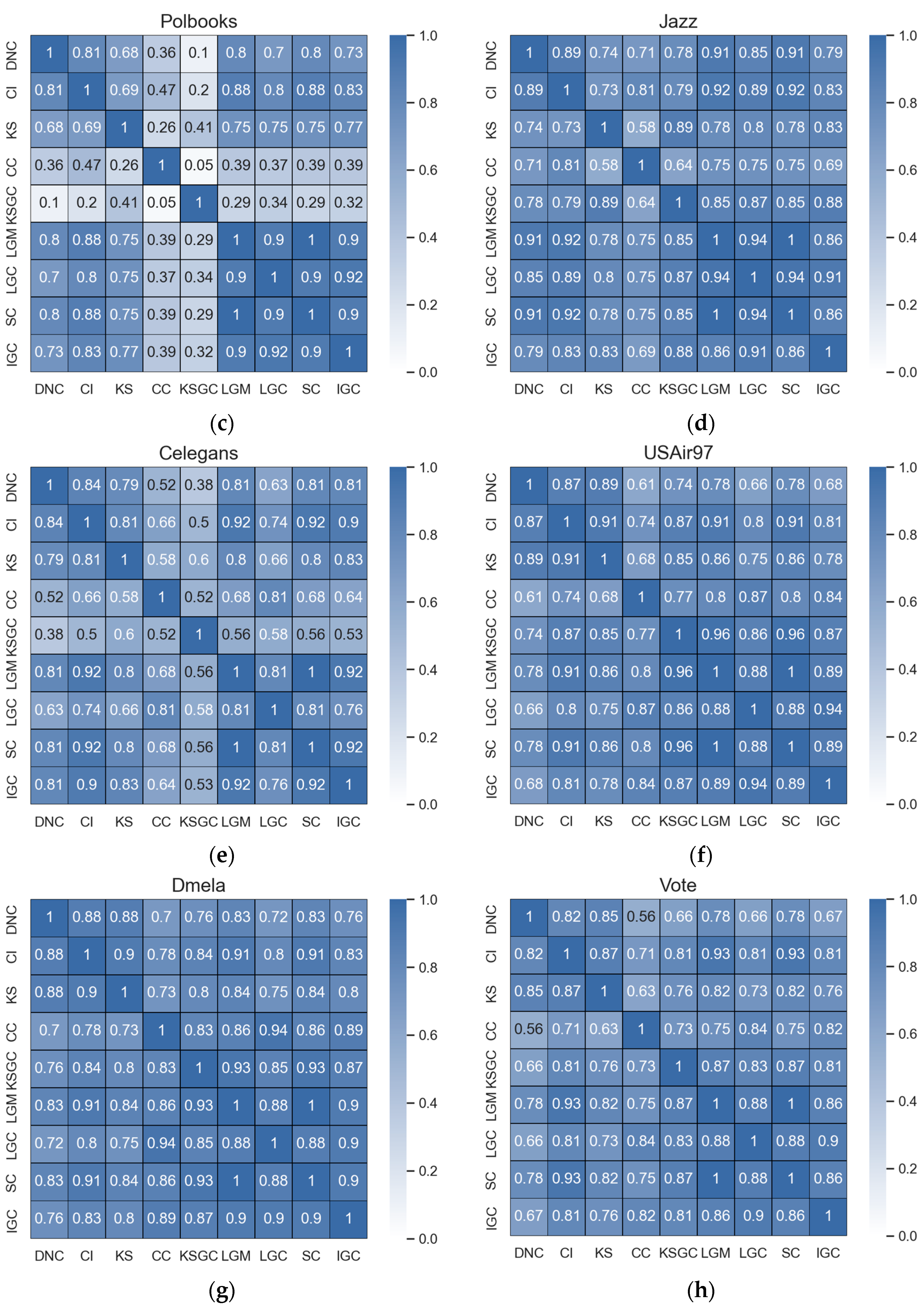
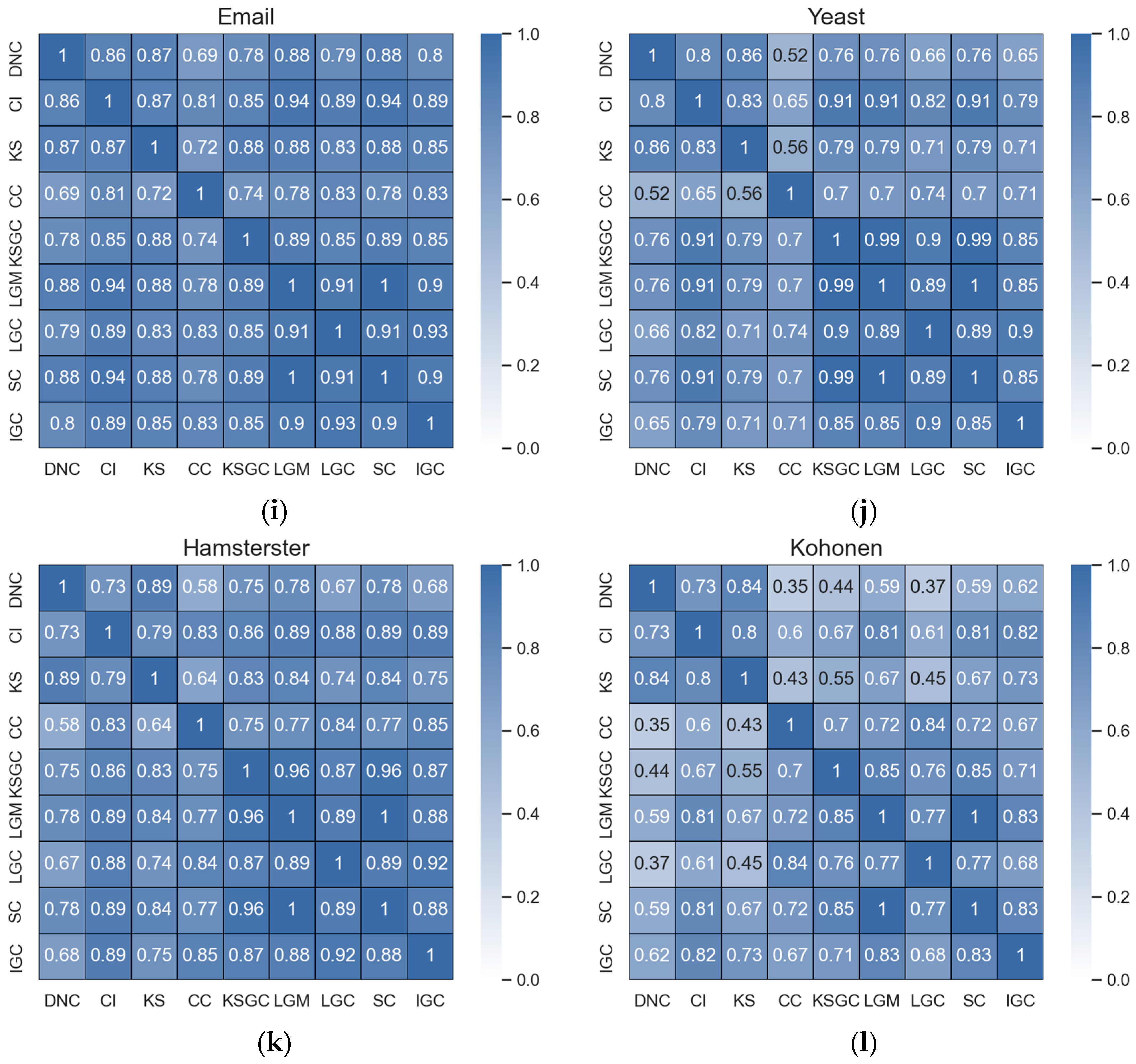
Figure 2.
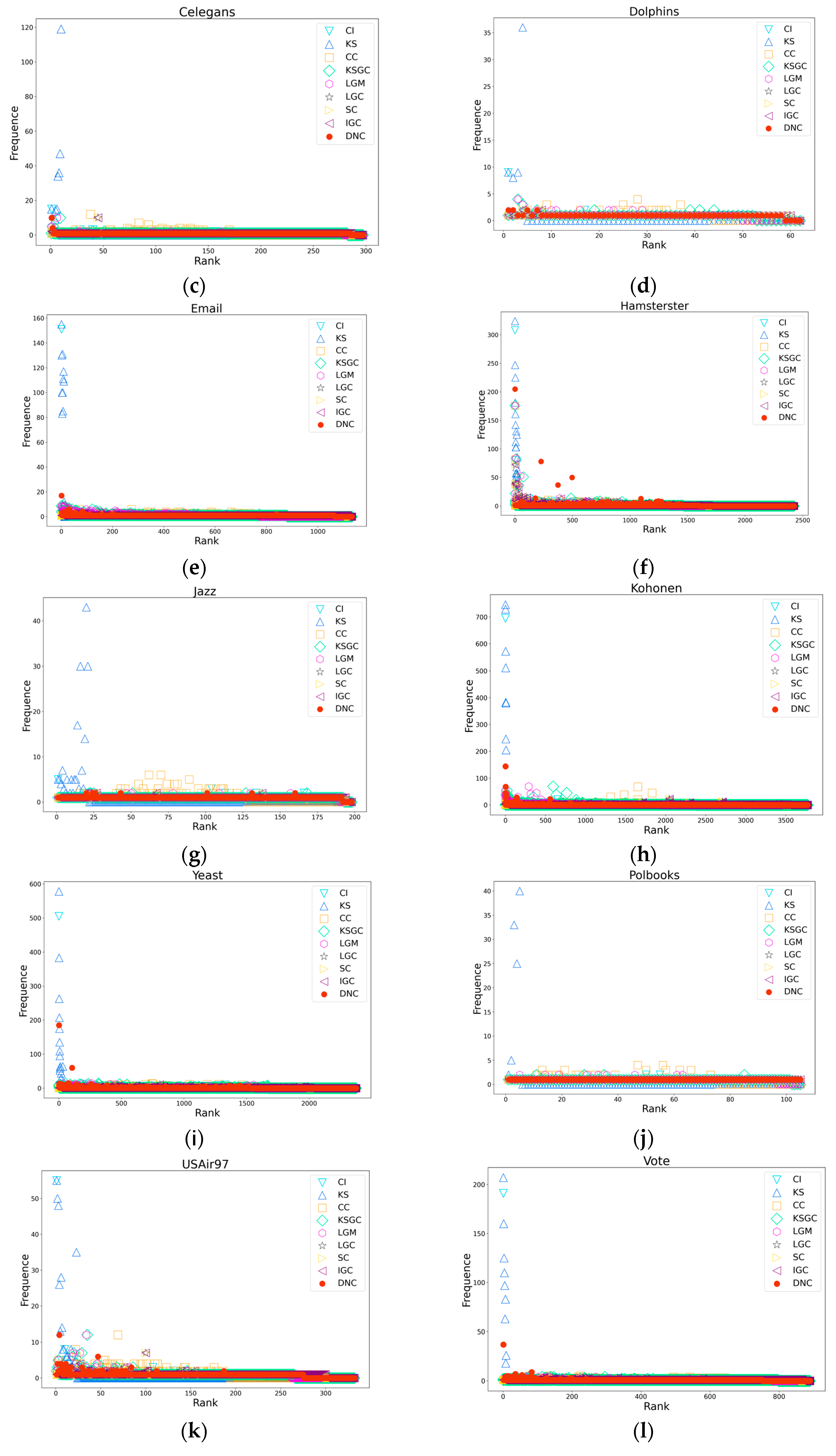
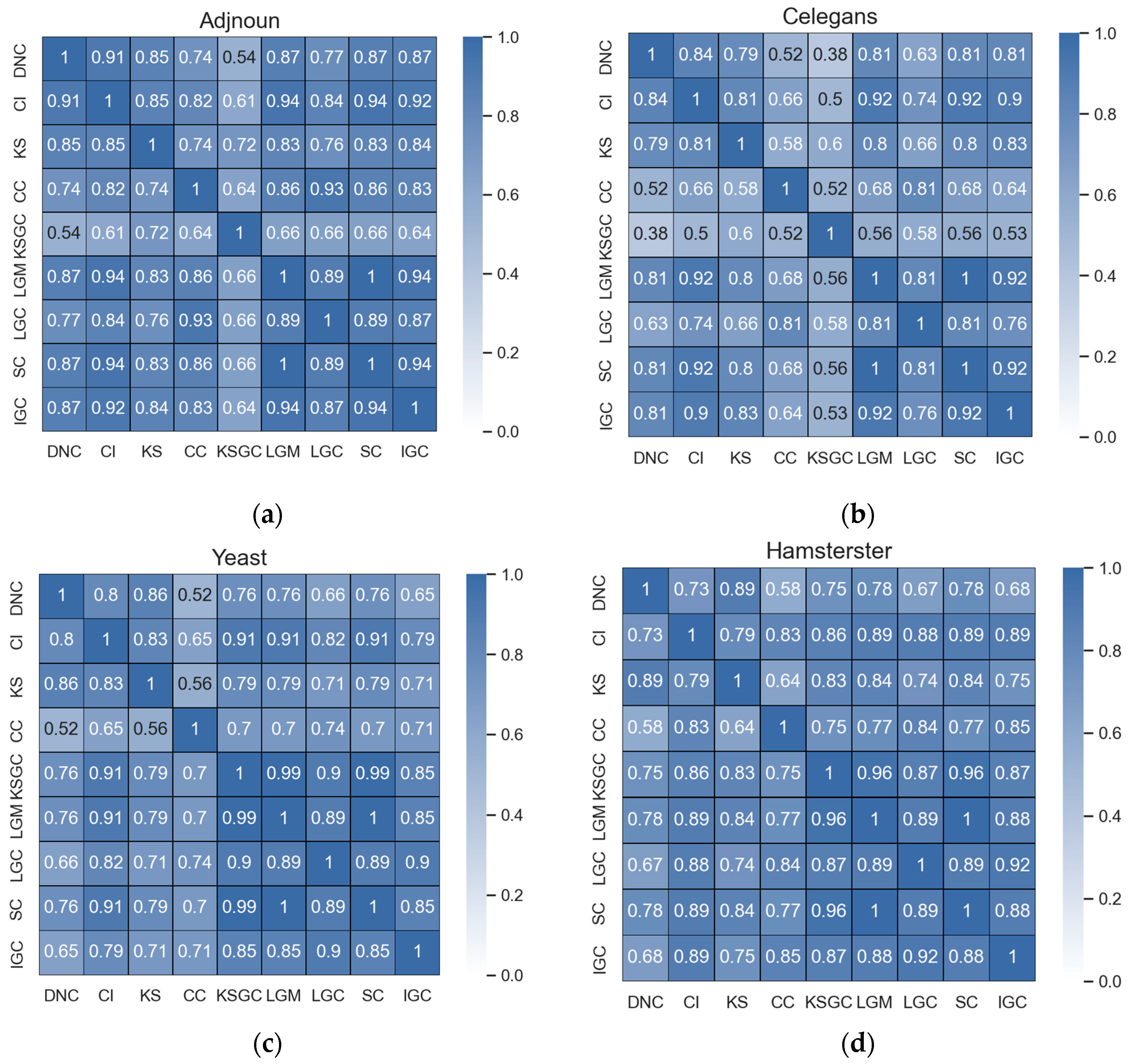
Subfigures (a–d) represent the correlation matrices between DNC and the baseline methods in the Adjnoun, Celegans, Yeast, and Hamsterster networks. The correlation coefficients between the two methods are mathematically expressed by the corresponding rows and columns. The first row represents the correlation coefficients between DNC and the baseline methods, while the second row represents the correlation coefficients between CI and the remaining methods. The black numbers in the figure indicate that the two methods have low correlation.
Figure 2.
Subfigures (a–d) represent the correlation matrices between DNC and the baseline methods in the Adjnoun, Celegans, Yeast, and Hamsterster networks. The correlation coefficients between the two methods are mathematically expressed by the corresponding rows and columns. The first row represents the correlation coefficients between DNC and the baseline methods, while the second row represents the correlation coefficients between CI and the remaining methods. The black numbers in the figure indicate that the two methods have low correlation.
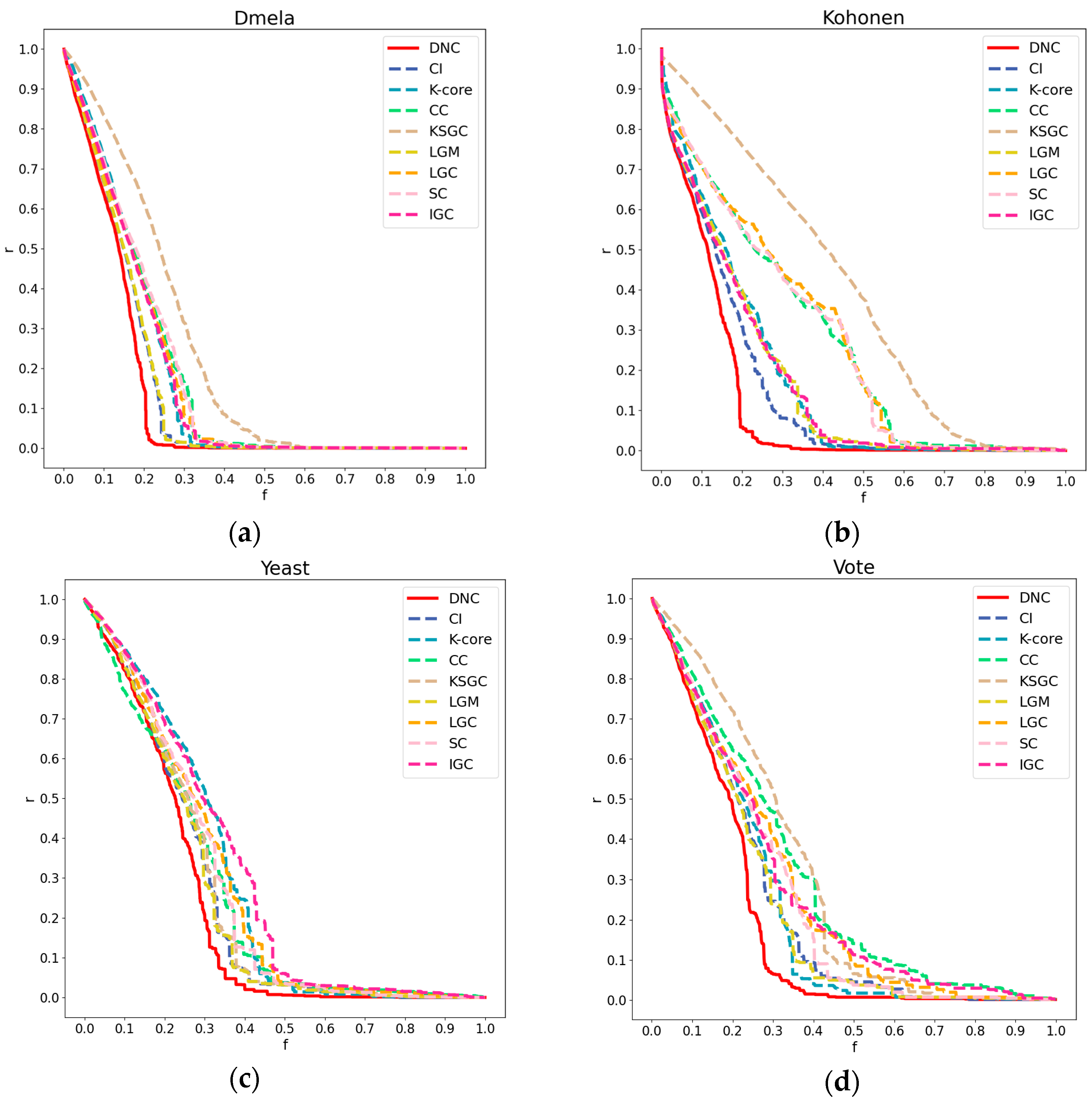
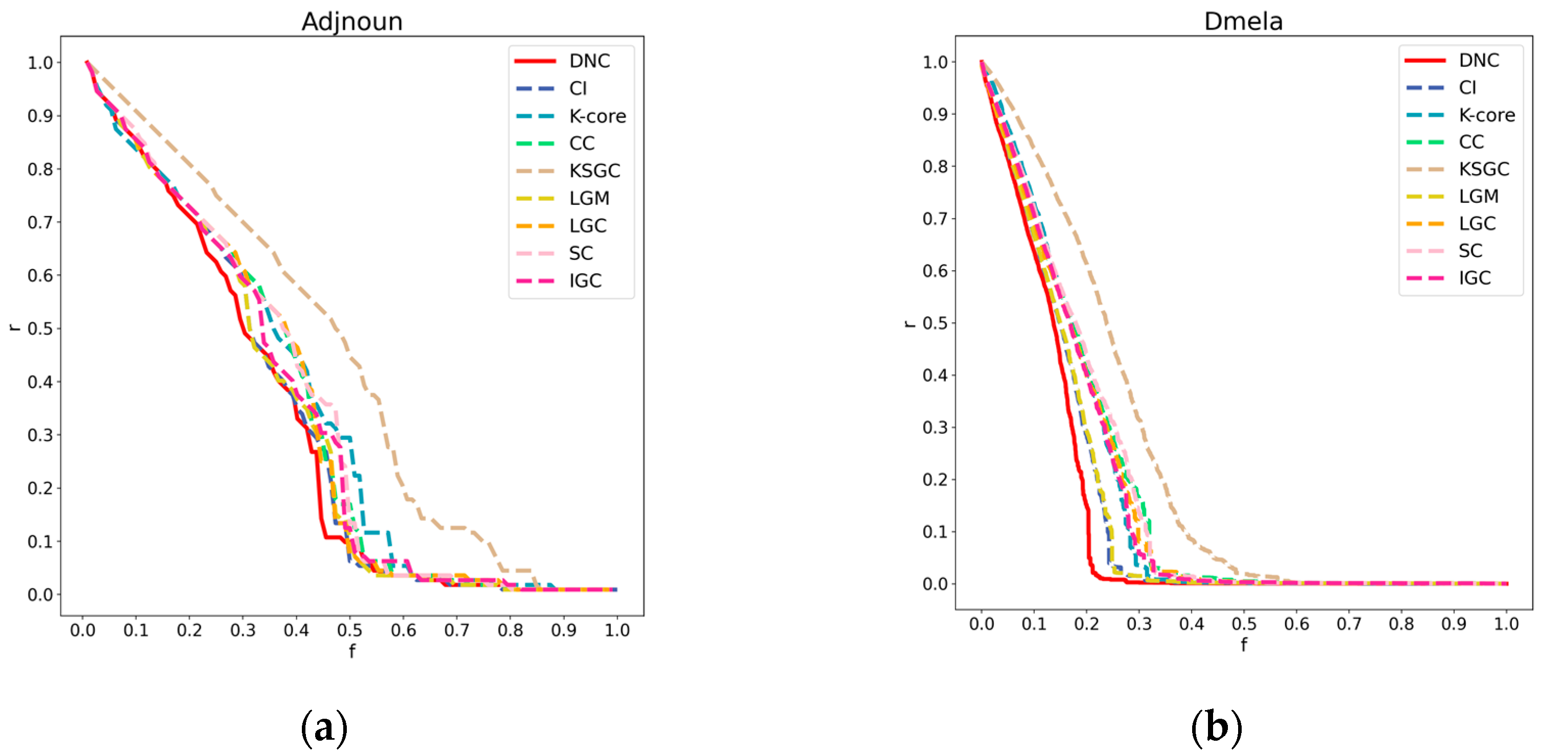
Figure 3.
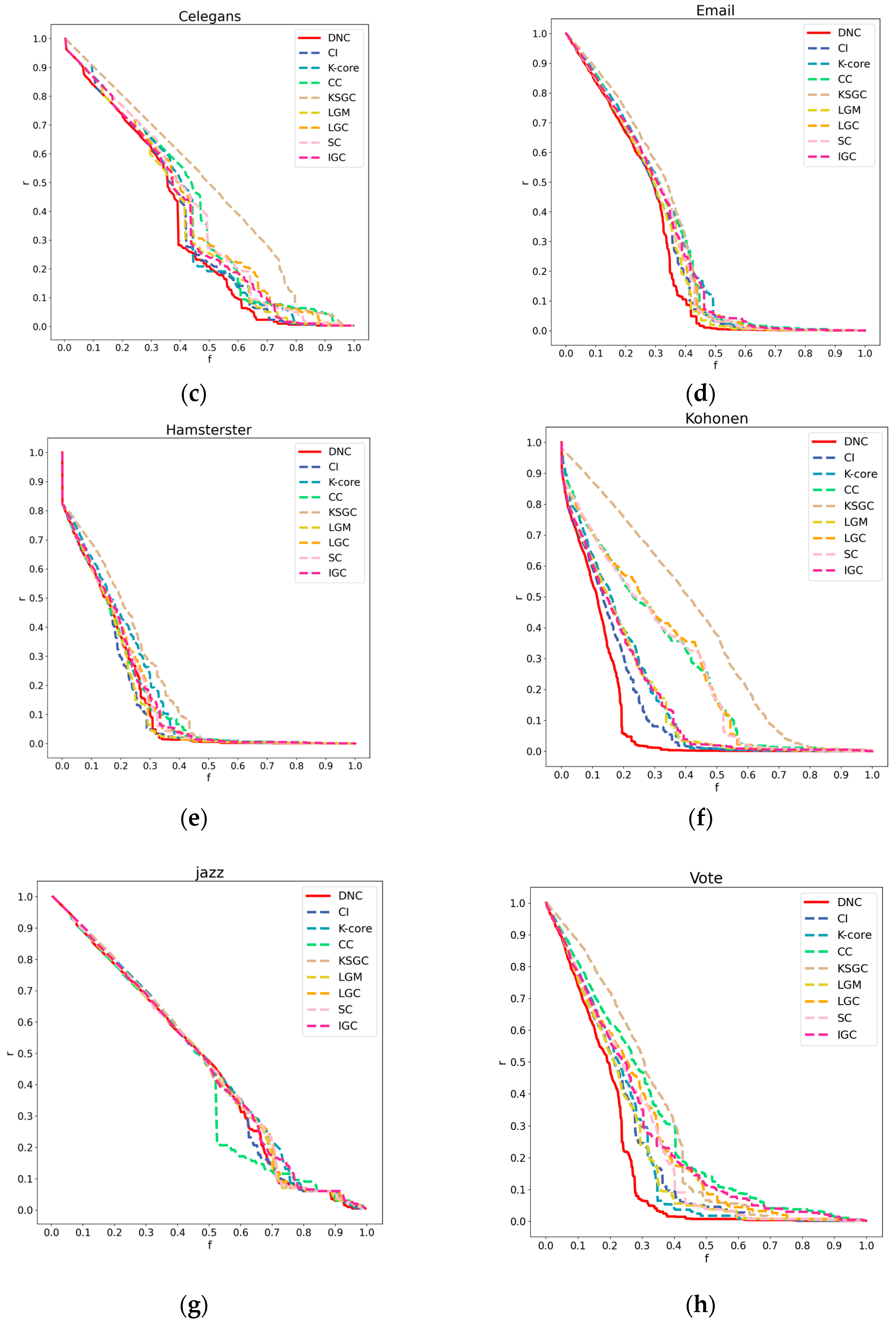
Subfigures (a), (b), (c), and (d) respectively represent the performance of DNC and the baseline methods in terms of accuracy on the Dmela, Kohonen, Yeast, and Vote networks. The x-axis of each subfigure represents the sequential removal of nodes according to DNC or the baseline methods. The y-axis measures the degree of network collapse, with a faster descent indicating greater accuracy for the method.
Figure 3.
Subfigures (a), (b), (c), and (d) respectively represent the performance of DNC and the baseline methods in terms of accuracy on the Dmela, Kohonen, Yeast, and Vote networks. The x-axis of each subfigure represents the sequential removal of nodes according to DNC or the baseline methods. The y-axis measures the degree of network collapse, with a faster descent indicating greater accuracy for the method.
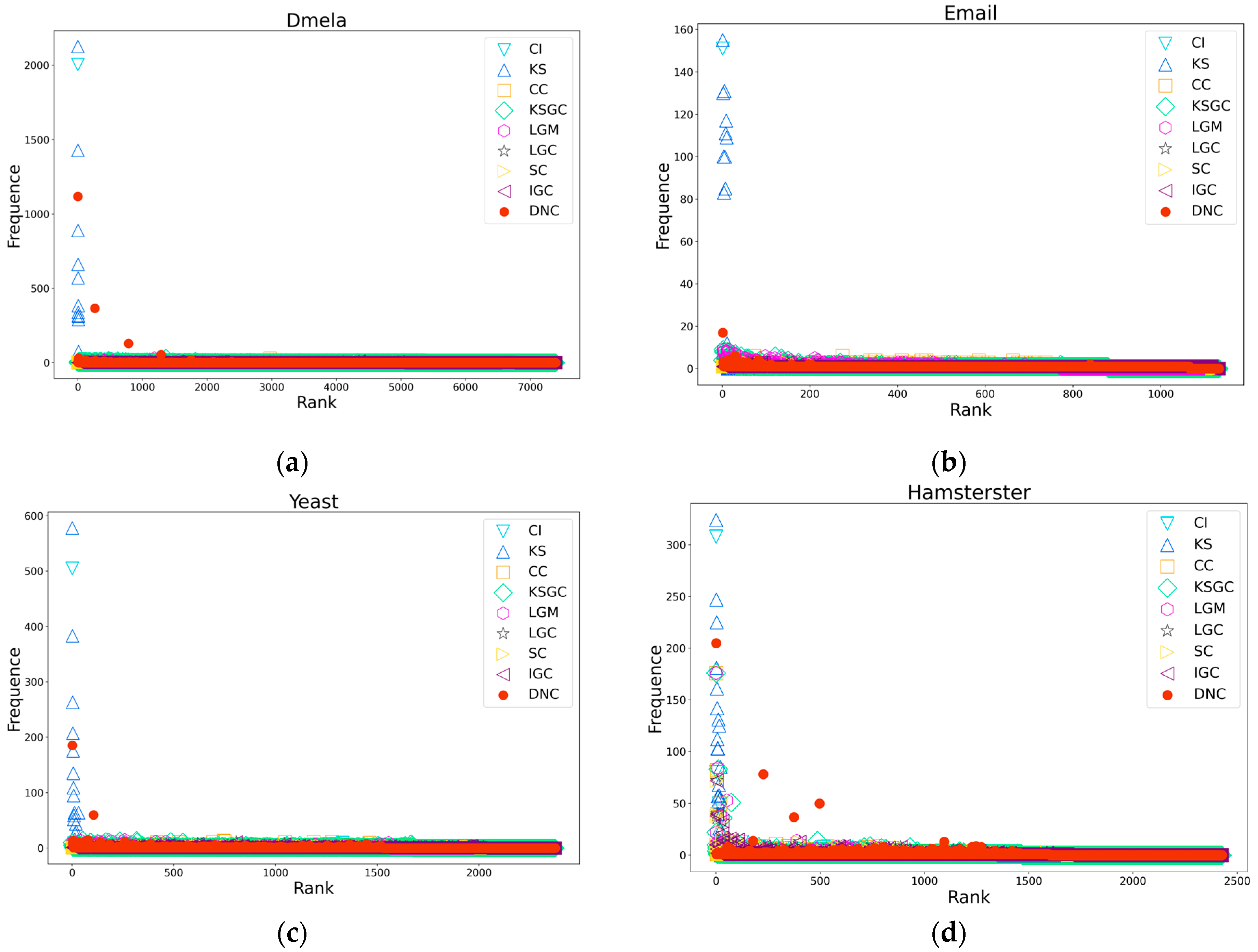
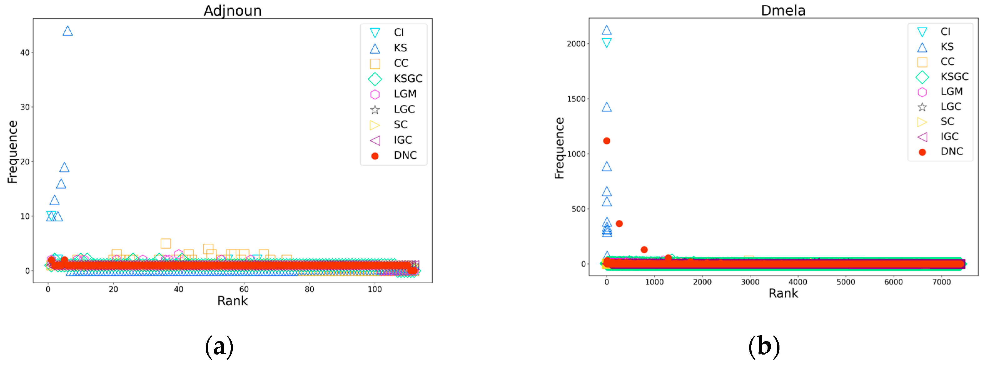
Figure 4.
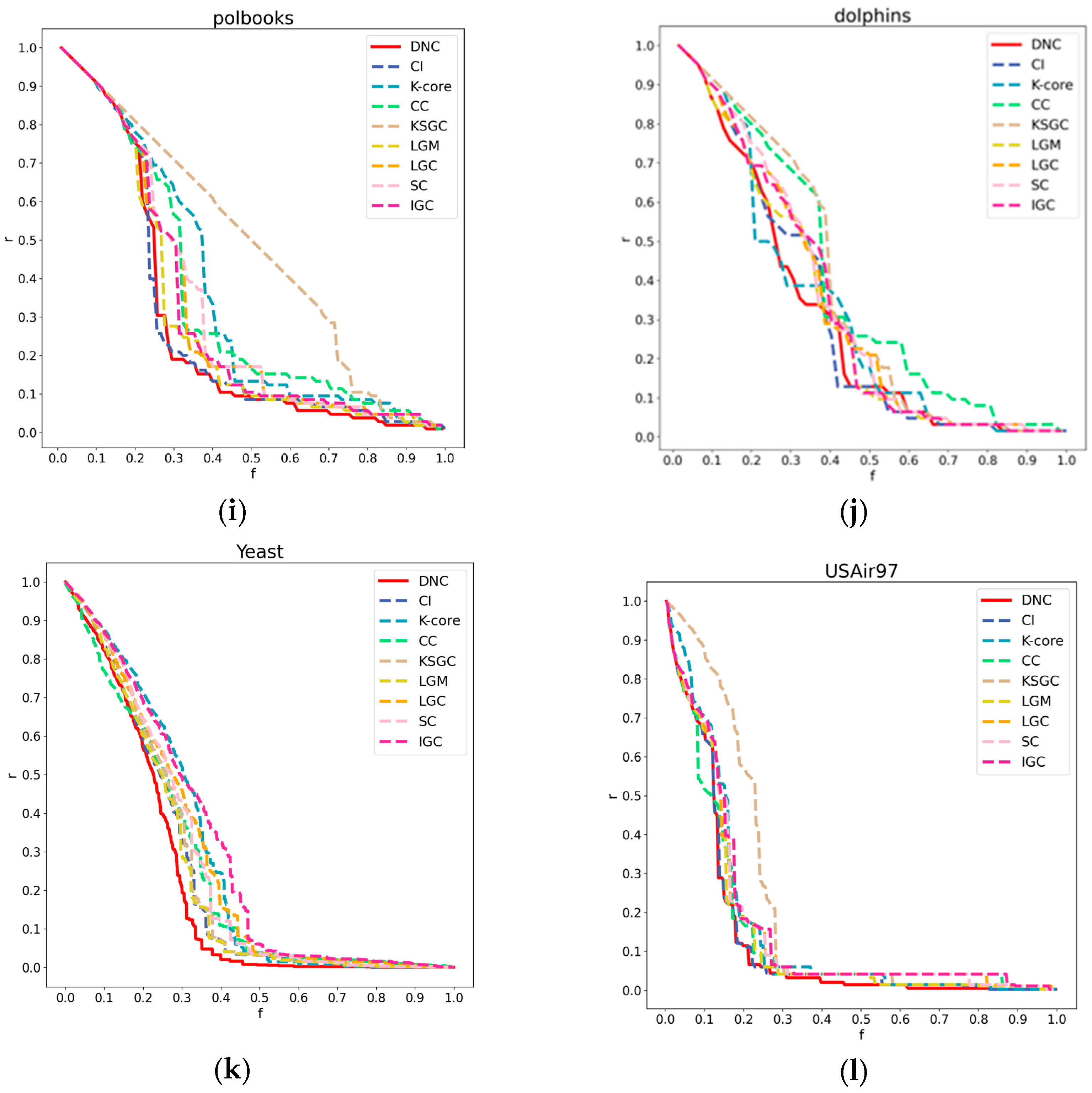
Subfigures (a), (b), (c), and (d) respectively depict the rank distribution plots of DNC and the baseline methods on the Dmela, Email, Yeast, and Hamsterster networks. The x-axis of each subfigure represents the ranking of nodes, while the y-axis represents the count of nodes with the same ranking.
Figure 4.
Subfigures (a), (b), (c), and (d) respectively depict the rank distribution plots of DNC and the baseline methods on the Dmela, Email, Yeast, and Hamsterster networks. The x-axis of each subfigure represents the ranking of nodes, while the y-axis represents the count of nodes with the same ranking.
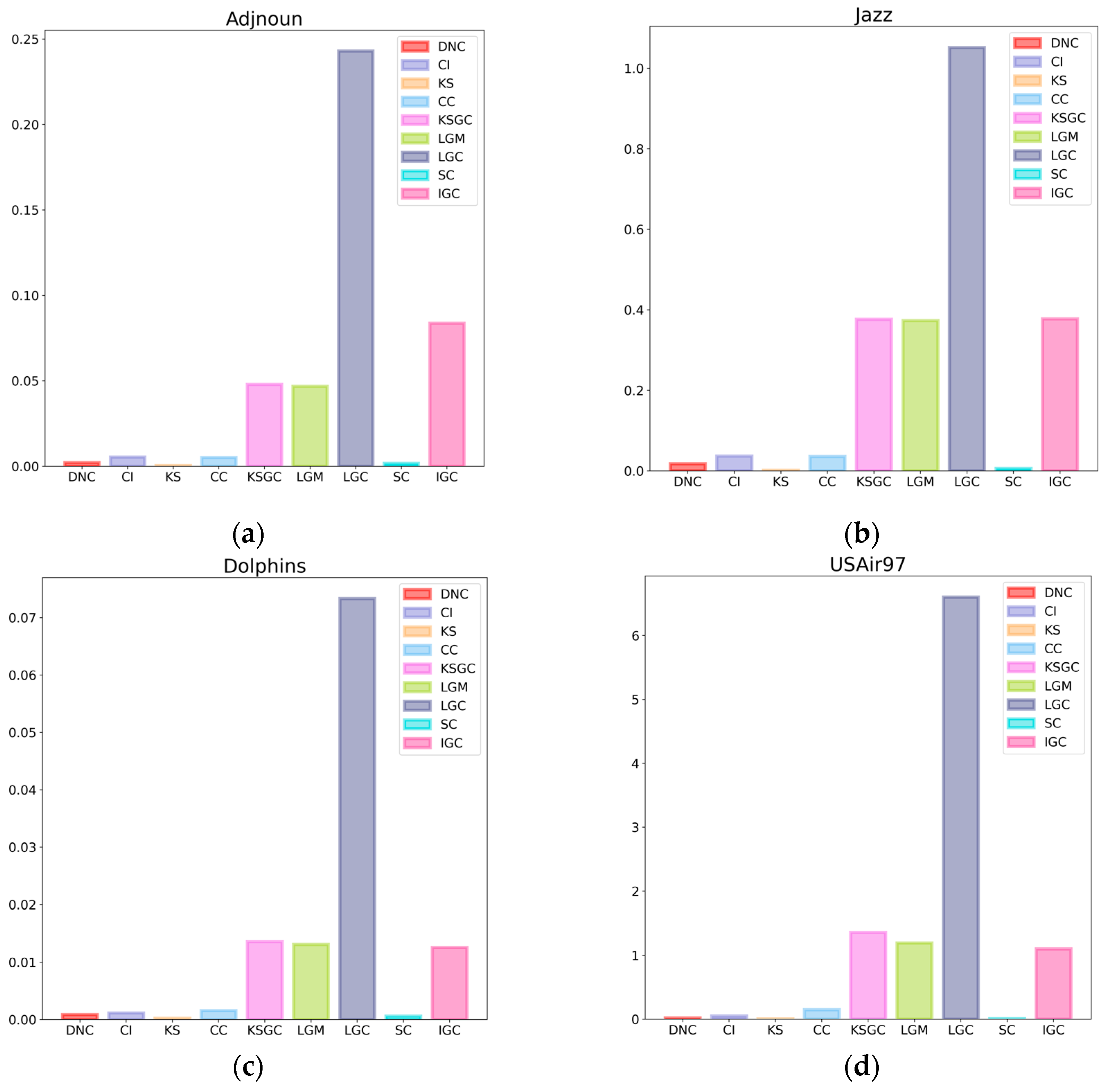
Figure 5.
Subfigures (a), (b), (c), and (d) respectively illustrate the CPU time comparison between DNC and the baseline methods on the Adjnoun, Jazz, Dolphins, and USAir97 networks.
Figure 5.
Subfigures (a), (b), (c), and (d) respectively illustrate the CPU time comparison between DNC and the baseline methods on the Adjnoun, Jazz, Dolphins, and USAir97 networks.
Figure 6.
Performance comparison of DNC and the baseline methods on the BA network.
Figure 6.
Performance comparison of DNC and the baseline methods on the BA network.
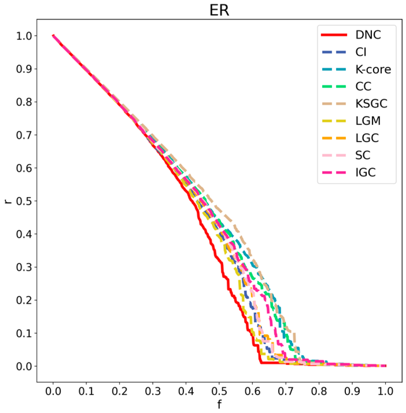
Figure 7.
Performance comparison of DNC and the baseline methods on the ER network.
Figure 7.
Performance comparison of DNC and the baseline methods on the ER network.
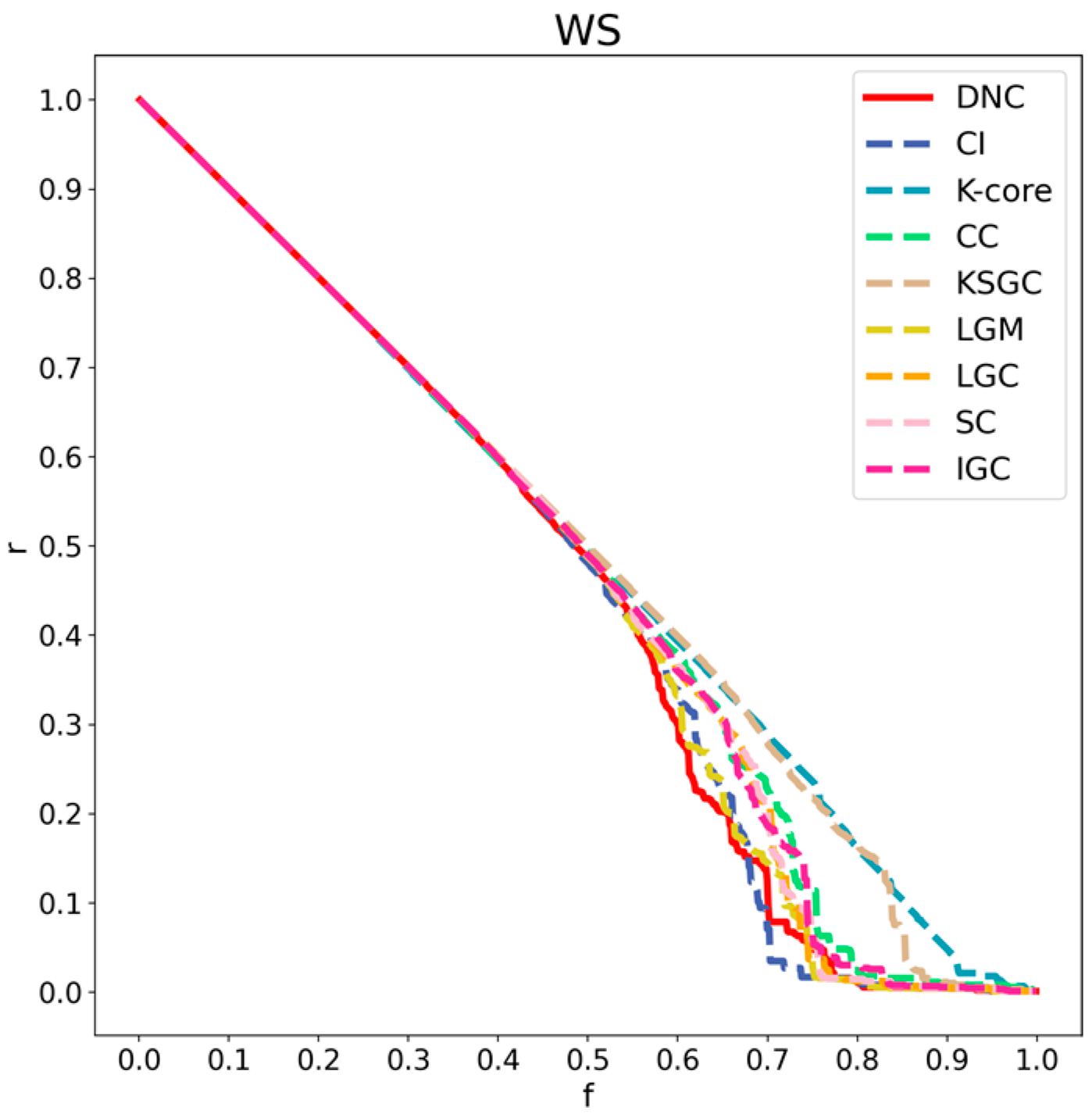
Figure 8.
Performance comparison of DNC and the baseline methods on the WS network.
Figure 8.
Performance comparison of DNC and the baseline methods on the WS network.
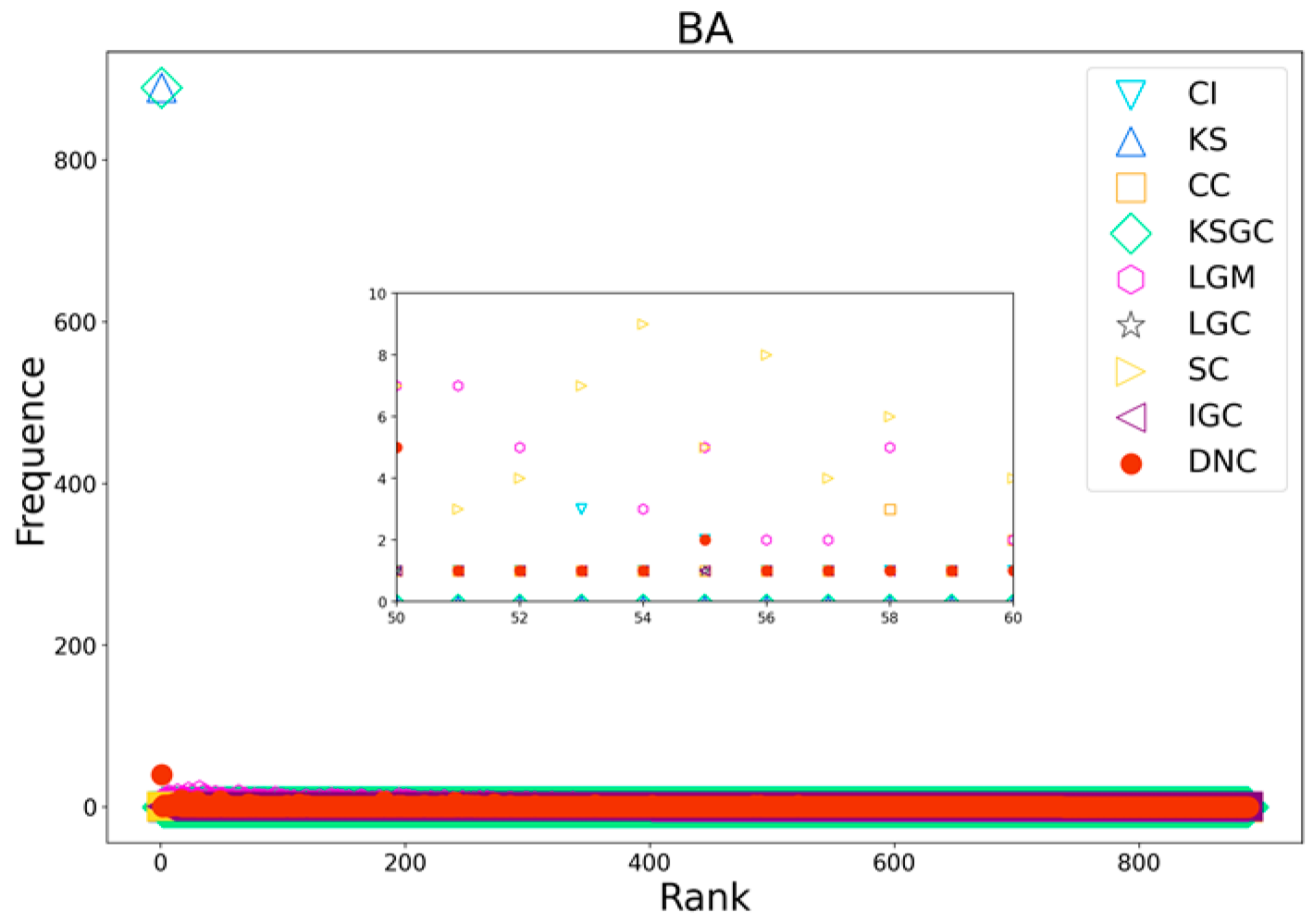
Figure 9.
Rank distribution plots of DNC and the baseline methods on BA networks.
Figure 9.
Rank distribution plots of DNC and the baseline methods on BA networks.
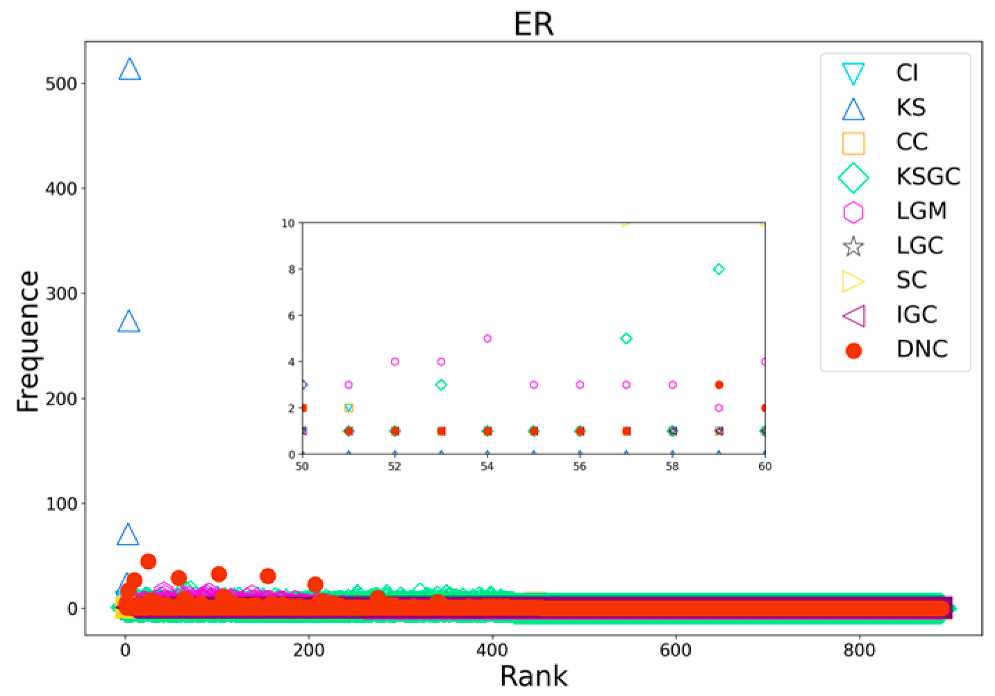
Figure 10.
Rank distribution plots of DNC and the baseline methods on ER networks.
Figure 10.
Rank distribution plots of DNC and the baseline methods on ER networks.
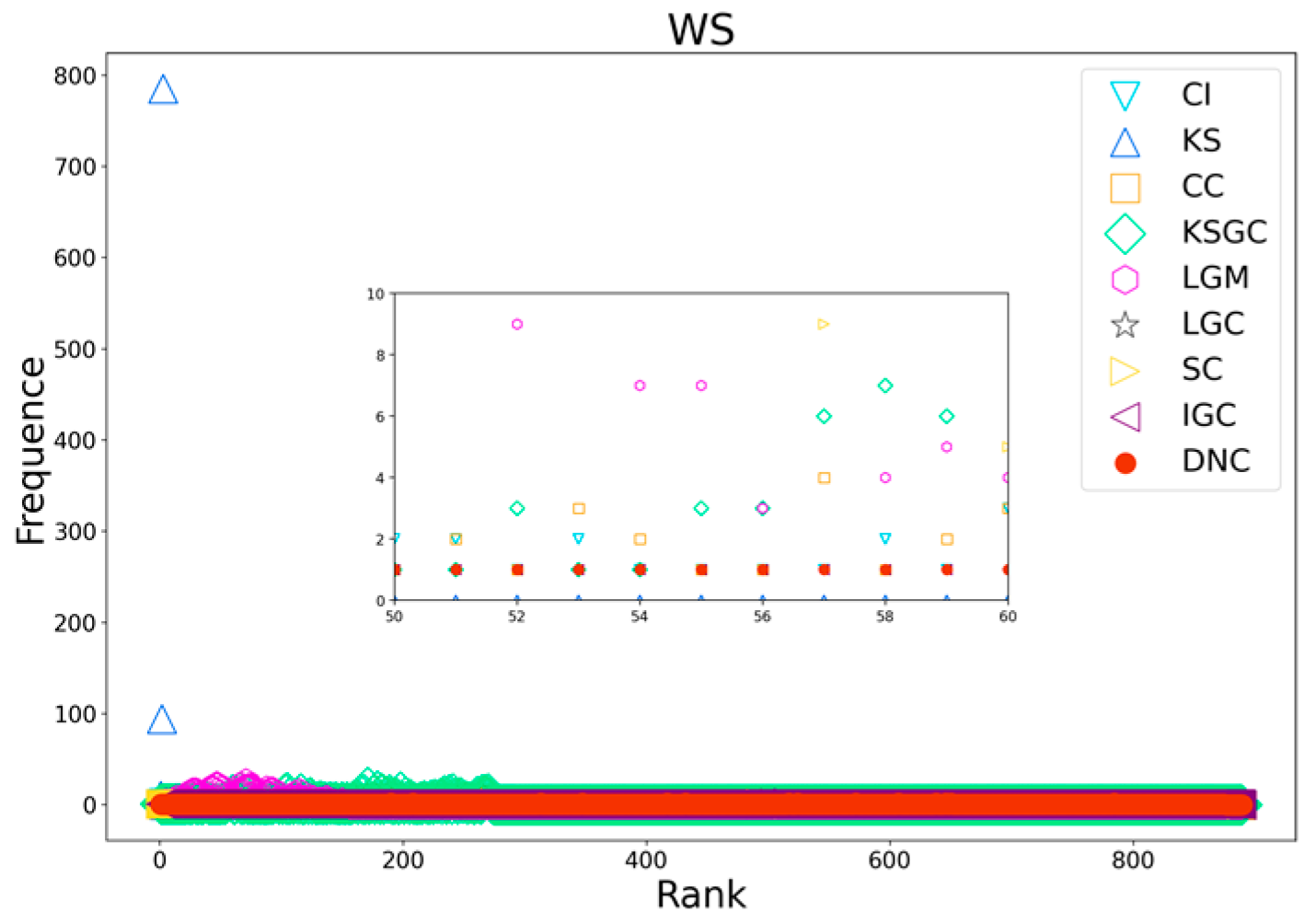
Figure 11.
Rank distribution plots of DNC and the baseline methods on WS networks.
Figure 11.
Rank distribution plots of DNC and the baseline methods on WS networks.
Table 1.
The LCC of the first-order neighbors of node 8 in the Karate network.
Table 1.
The LCC of the first-order neighbors of node 8 in the Karate network.
| Node | 0 | 2 | 30 | 32 | 33 |
| LCC | 0.15 | 0.24 | 0.50 | 0.20 | 0.11 |
Table 2.
Top ten nodes with DNC compared to baseline methods.
Table 2.
Top ten nodes with DNC compared to baseline methods.
| DNC | CI | KS | CC | KSGC | LGM | LGC | SC | IGC |
|---|
| 33 | 0 | 0 | 0 | 8 | 33 | 33 | 0 | 0 |
| 0 | 33 | 1 | 2 | 13 | 0 | 0 | 33 | 33 |
| 32 | 32 | 2 | 33 | 30 | 32 | 32 | 2 | 2 |
| 1 | 2 | 3 | 31 | 7 | 2 | 2 | 32 | 32 |
| 2 | 1 | 7 | 8 | 3 | 1 | 1 | 8 | 1 |
| 3 | 31 | 8 | 13 | 19 | 31 | 8 | 13 | 3 |
| 31 | 3 | 13 | 32 | 31 | 8 | 13 | 1 | 8 |
| 13 | 8 | 30 | 19 | 19 | 13 | 31 | 31 | 13 |
| 23 | 13 | 32 | 1 | 23 | 3 | 23 | 3 | 31 |
| 5 | 30 | 33 | 3 | 27 | 23 | 3 | 30 | 30 |
| 33 | 0 | 0 | 0 | 8 | 33 | 33 | 0 | 0 |
| 0 | 33 | 1 | 2 | 13 | 0 | 0 | 33 | 33 |
| 32 | 32 | 2 | 33 | 30 | 32 | 32 | 2 | 2 |
| 1 | 2 | 3 | 31 | 7 | 2 | 2 | 32 | 32 |
Table 3.
The typical metric values for these 12 networks. The structural parameters and topological properties of all of these networks, including the number of nodes and edges , average degree , maximum degree , clustering coefficient , and assortativity coefficient .
Table 3.
The typical metric values for these 12 networks. The structural parameters and topological properties of all of these networks, including the number of nodes and edges , average degree , maximum degree , clustering coefficient , and assortativity coefficient .
| Network | | | | | | |
|---|
| Dolphins | 62 | 159 | 5 | 12 | 0.2590 | −0.0436 |
| Polbooks | 105 | 441 | 8 | 25 | 0.4875 | −0.1279 |
| Adjnoun | 112 | 425 | 7 | 49 | 0.1728 | −0.1293 |
| Jazz | 198 | 2742 | 27 | 100 | 0.5203 | 0.0202 |
| C_elegans | 297 | 2148 | 15 | 134 | 0.3115 | −0.1520 |
| USAir97 | 332 | 2126 | 12 | 139 | 0.6252 | −0.2079 |
| Vote | 889 | 2914 | 7 | 102 | 0.1528 | −0.0288 |
| Email | 1133 | 5451 | 9 | 71 | 0.2200 | 0.0782 |
| Yeast | 2375 | 11,693 | 9 | 118 | 0.3100 | 0.4539 |
| Hamsterster | 2426 | 16,630 | 14 | 273 | 0.5375 | 0.0474 |
| Kohonen | 3772 | 12,718 | 5 | 740 | 0.2100 | −0.1204 |
| Dmela | 7393 | 25,569 | 6 | 190 | 0.0118 | −0.0465 |
Table 4.
The robustness values (R) of DNC and the baseline methods across the different datasets show that, in the majority of networks, DNC exhibits the least robustness. The smallest R values in the different networks are shown in bold.
Table 4.
The robustness values (R) of DNC and the baseline methods across the different datasets show that, in the majority of networks, DNC exhibits the least robustness. The smallest R values in the different networks are shown in bold.
| Network | DNC | CI | KS | CC | KSGC | LGM | LGC | SC | IGC |
|---|
| Dolphins | 0.2862 | 0.2882 | 0.2947 | 0.3548 | 0.3005 | 0.3033 | 0.3153 | 0.3122 | 0.3124 |
| Polbooks | 0.2604 | 0.2669 | 0.3481 | 0.3341 | 0.2787 | 0.2796 | 0.3042 | 0.3146 | 0.2994 |
| Adjnoun | 0.2913 | 0.3025 | 0.3308 | 0.3260 | 0.3096 | 0.3050 | 0.3252 | 0.3276 | 0.3166 |
| Jazz | 0.4399 | 0.4384 | 0.4559 | 0.4201 | 0.4459 | 0.4438 | 0.4470 | 0.4463 | 0.4488 |
| C_elegans | 0.3311 | 0.3480 | 0.3689 | 0.3960 | 0.3534 | 0.3563 | 0.3849 | 0.3849 | 0.3646 |
| USAir97 | 0.1230 | 0.1300 | 0.1546 | 0.1367 | 0.1379 | 0.1414 | 0.1508 | 0.1525 | 0.1562 |
| Vote | 0.1781 | 0.2188 | 0.2200 | 0.2954 | 0.3000 | 0.2169 | 0.2623 | 0.2418 | 0.2641 |
| Email | 0.2573 | 0.2702 | 0.2935 | 0.2893 | 0.2699 | 0.2710 | 0.2846 | 0.2828 | 0.2890 |
| Yeast | 0.2203 | 0.2368 | 0.2833 | 0.2500 | 0.2414 | 0.2452 | 0.2772 | 0.2704 | 0.2953 |
| Hamsterster | 0.1487 | 0.1422 | 0.1760 | 0.1605 | 0.1997 | 0.1461 | 0.1621 | 0.1604 | 0.1624 |
| Kohonen | 0.1085 | 0.1424 | 0.1708 | 0.2683 | 0.3908 | 0.1676 | 0.2722 | 0.2661 | 0.1674 |
| Dmela | 0.1293 | 0.1423 | 0.1681 | 0.1746 | 0.1463 | 0.1486 | 0.1789 | 0.1774 | 0.1673 |
Table 5.
The M value of DNC and the baseline methods. The largest M values in the different networks are shown in bold.
Table 5.
The M value of DNC and the baseline methods. The largest M values in the different networks are shown in bold.
| Network | DNC | CI | KS | CC | KSGC | LGM | LGC | SC | IGC |
|---|
| Dolphins | 0.9958 | 0.9613 | 0.3769 | 0.9737 | 0.9852 | 0.9821 | 0.9979 | 0.9675 | 0.3124 |
| Polbooks | 1.0000 | 0.9993 | 0.4949 | 0.9847 | 0.9985 | 0.9967 | 1.0000 | 0.9887 | 1.0000 |
| Adjnoun | 0.9994 | 0.9846 | 0.5990 | 0.9837 | 0.9981 | 0.9961 | 1.0000 | 0.9920 | 0.9997 |
| Jazz | 0.9993 | 0.9980 | 0.7944 | 0.9878 | 0.9994 | 0.9991 | 0.9996 | 0.9983 | 0.9994 |
| C_elegans | 0.9977 | 0.9949 | 0.6094 | 0.9893 | 0.9974 | 0.9972 | 0.9979 | 0.9955 | 0.9977 |
| USAir97 | 0.9951 | 0.9433 | 0.8114 | 0.9892 | 0.9935 | 0.9933 | 0.9981 | 0.9928 | 0.9951 |
| Vote | 0.9956 | 0.9100 | 0.7265 | 0.9988 | 0.9994 | 0.9993 | 0.9999 | 0.9887 | 0.9997 |
| Email | 0.9993 | 0.9649 | 0.8088 | 0.9988 | 0.9982 | 0.9977 | 0.9999 | 0.9943 | 0.9999 |
| Yeast | 0.9856 | 0.9111 | 0.7737 | 0.9988 | 0.9988 | 0.9986 | 0.9996 | 0.9873 | 0.9992 |
| Hamsterster | 0.9819 | 0.9641 | 0.8714 | 0.9851 | 0.9848 | 0.9844 | 0.9957 | 0.9829 | 0.9857 |
| Kohonen | 0.9954 | 0.9332 | 0.7306 | 0.9980 | 0.9965 | 0.9960 | 0.9997 | 0.9943 | 0.9984 |
| Dmela | 0.9491 | 0.8583 | 0.7083 | 0.9996 | 0.9996 | 0.9995 | 0.9999 | 0.9905 | 0.9998 |
| Average | 0.9914 | 0.9533 | 0.6883 | 0.9908 | 0.9957 | 0.9950 | 0.9988 | 0.9879 | 0.9414 |
Table 6.
CPU running time of DNC and the baseline methods across different datasets.
Table 6.
CPU running time of DNC and the baseline methods across different datasets.
| Network | DNC | CI | KS | CC | KSGC | LGM | LGC | SC | IGC |
|---|
| Dolphins | 0.0008 | 0.0012 | 0.0002 | 0.0016 | 0.0136 | 0.0131 | 0.0733 | 0.0006 | 0.0126 |
| Polbooks | 0.0020 | 0.0039 | 0.0004 | 0.0043 | 0.0419 | 0.0412 | 0.3333 | 0.0034 | 0.0442 |
| Adjnoun | 0.0022 | 0.0054 | 0.0004 | 0.0052 | 0.0479 | 0.0469 | 0.2430 | 0.0017 | 0.0837 |
| Jazz | 0.0175 | 0.0368 | 0.0015 | 0.0359 | 0.3764 | 0.4438 | 1.0518 | 0.0063 | 0.3777 |
| C_elegans | 0.0110 | 0.0413 | 0.0015 | 0.0457 | 0.4396 | 0.4176 | 2.4965 | 0.0078 | 0.7293 |
| USAir97 | 0.0195 | 0.0520 | 0.0050 | 0.1501 | 1.3578 | 1.1940 | 6.6021 | 0.0084 | 1.1002 |
| Vote | 0.0206 | 0.0964 | 0.0046 | 0.6506 | 5.6010 | 5.5481 | 115.3479 | 0.0186 | 4.4040 |
| Email | 0.0294 | 0.1170 | 0.0045 | 0.6634 | 5.7952 | 5.7732 | 130.6723 | 0.0225 | 6.0688 |
| Yeast | 0.0736 | 0.1971 | 0.0105 | 3.1377 | 27.2292 | 27.7196 | 1832.8288 | 0.4662 | 9.3199 |
| Hamsterster | 0.1881 | 1.0533 | 0.0157 | 6.7333 | 44.7648 | 45.4922 | 3458.4607 | 0.6355 | 27.4336 |
| Kohonen | 0.3810 | 3.7765 | 0.0425 | 23.3436 | 137.8985 | 139.2541 | 138,334.9177 | 0.5790 | 243.8257 |
| Dmela | 0.1596 | 3.0046 | 0.1210 | 141.5445 | 615.0009 | 597.0216 | 342,162.0082 | 0.1133 | 268.1242 |
Table 7.
Robustness of DNC and the baseline methods on the BA, WS, and ER networks.
Table 7.
Robustness of DNC and the baseline methods on the BA, WS, and ER networks.
| Network | DNC | CI | KS | CC | KSGC | LGM | LGC | SC | IGC |
|---|
| BA | 0.1973 | 0.2323 | 0.2937 | 0.3323 | 0.2937 | 0.2410 | 0.3209 | 0.3094 | 0.2467 |
| WS | 0.4385 | 0.4395 | 0.4867 | 0.4595 | 0.4831 | 0.4438 | 0.4532 | 0.4538 | 0.4562 |
| ER | 0.3771 | 0.3989 | 0.4305 | 0.4239 | 0.4390 | 0.3914 | 0.4053 | 0.4061 | 0.4157 |
Table 8.
Monotonicity indices of DNC and the baseline methods on BA, WS, and ER networks.
Table 8.
Monotonicity indices of DNC and the baseline methods on BA, WS, and ER networks.
| Network | DNC | CI | KS | CC | KSGC | LGM | LGC | SC | IGC |
|---|
| BA | 0.9810 | 0.9983 | 0.3183 | 0.9972 | 0.9944 | 0.9895 | 1.0000 | 0.9762 | 1.0000 |
| WS | 0.9999 | 0.9977 | 0.0438 | 0.9956 | 0.9873 | 0.9775 | 1.0000 | 0.9641 | 1.0000 |
| ER | 0.9691 | 0.9980 | 0.0579 | 0.9973 | 0.9937 | 0.9893 | 1.0000 | 0.9751 | 1.0000 |
Table 9.
CPU running time of DNC and the baseline methods on BA, WS, and ER networks.
Table 9.
CPU running time of DNC and the baseline methods on BA, WS, and ER networks.
| Network | DNC | CI | KS | CC | KSGC | LGM | LGC | SC | IGC |
|---|
| BA | 0.1627083 | 0.0640015 | 0.0034087 | 0.3464144 | 2.9167356 | 2.9463526 | 55.3866124 | 0.0902765 | 3.7456719 |
| WS | 0.1311109 | 0.0437059 | 0.0031796 | 0.3523955 | 3.2523763 | 3.2334455 | 66.9728192 | 0.1548067 | 2.9645162 |
| ER | 0.1070077 | 0.0406134 | 0.0034559 | 0.3901652 | 3.4885044 | 3.5960308 | 59.9473234 | 0.0861778 | 2.3780626 |


