CasOmniMVS: Cascade Omnidirectional Depth Estimation with Dynamic Spherical Sweeping

Abstract

Estimating 360${}^{\circ }$ depth from multiple cameras has been a challenging problem. However, existing methods often adopt a fixed-step spherical sweeping approach with densely sampled spheres and use numerous 3D convolutions in networks, which limits the speed of algorithms in practice. Additionally, obtaining high-precision depth maps of real scenes poses a challenge for the existing algorithms. In this paper, we design a cascade architecture using a dynamic spherical sweeping method that progressively refines the depth estimation from coarse to fine over multiple stages. The proposed method adaptively adjusts sweeping intervals and ranges based on the predicted depth and the uncertainty from the previous stage, resulting in a more efficient cost aggregation performance. The experimental results demonstrated that our method achieved state-of-the-art accuracy with reduced GPU memory usage and time consumption compared to the other methods. Furthermore, we illustrate that our method achieved satisfactory performance on real-world data, despite being trained on synthetic data, indicating its generalization potential and practical applicability.

1. Introduction

Estimating 360° depth information from images is a fundamental task in computer vision. In recent years, image-based depth estimation techniques have made significant progress. These methods, including binocular stereo matching and multi-view dense reconstruction, use deep learning to analyze images with a limited field of view, restricting the output depth to a specific view. However, omnidirectional depth estimation ability is required for applications including autonomous driving and robot navigation, to perceive the surrounding environment. One potential approach is to apply binocular stereo matching to images captured at different views, thereby estimating scene depth individually for each view. Similarly to the process of panoramic image stitching, we can perform depth image stitching by combining images captured from various perspectives to create a panoramic depth image. However, the depth at the stitching seam is discontinuous and requires additional post-processing for smoothing. This approach increases the complexity, as it requires many sets of binocular cameras and also requires stereo rectification. To tackle these challenges, several omnidirectional depth estimation algorithms have been proposed.

Unlike traditional methods limited to a narrow FOV, omnidirectional depth estimation aims to overcome this limitation by generating surround depth. Several existing methods [1,2,3,4] adopt ideas from monocular depth estimation, directly predicting depth from individual panoramic images. While simplifying system hardware requirements, the limited input information risks inaccurate results in certain contexts, particularly those involving distant or heavily occluded objects. Other methods [5,6,7] incorporate conventional binocular stereo matching constraints and epipolar geometry into panoramic image pairs, predicting more reliable depth. Nevertheless, the practical applicability remains limited due to challenges in obtaining such panoramas and additional calibration requirements.

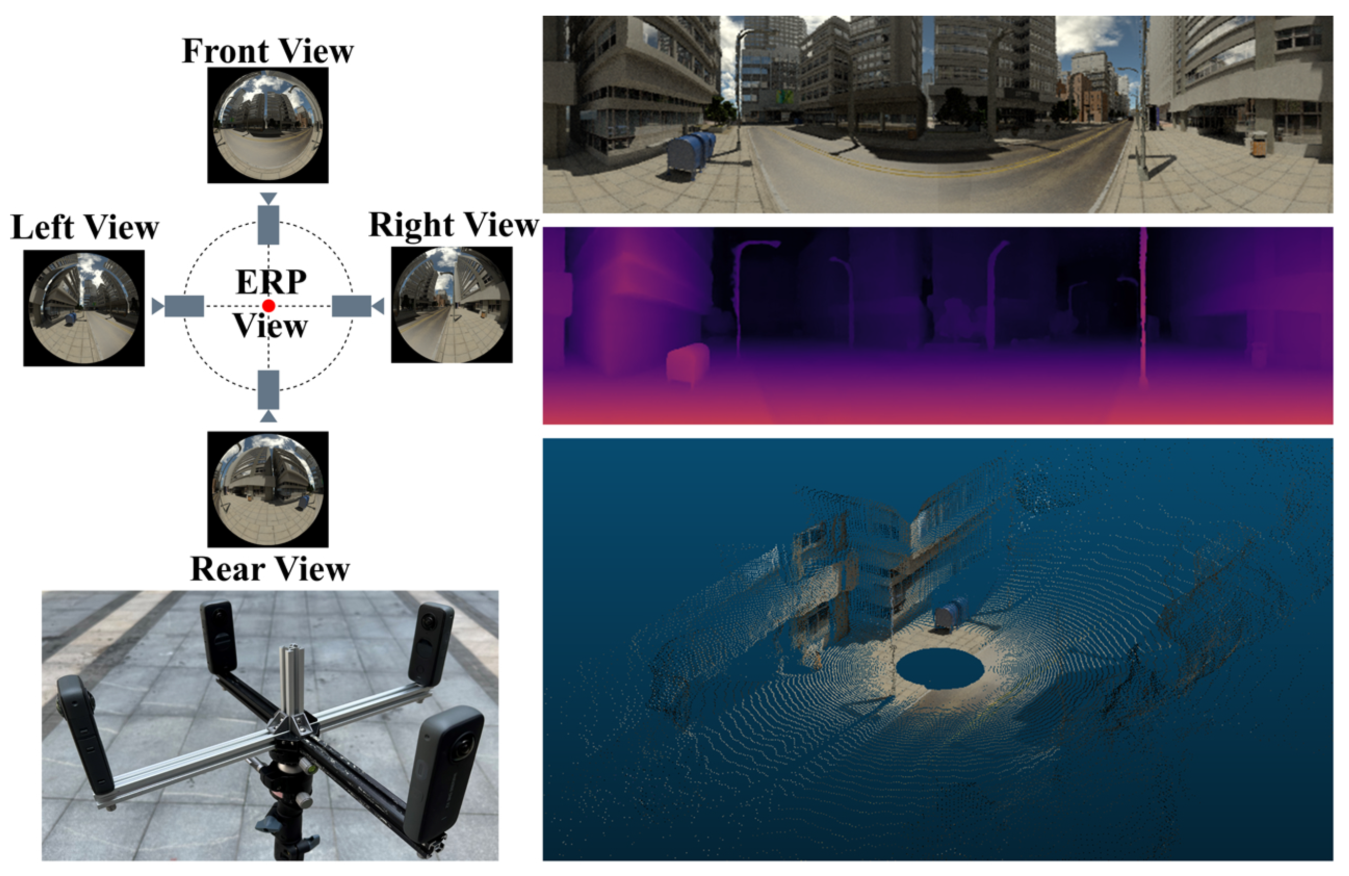
Some methods [8,9] use fisheye images to directly estimate omnidirectional depth by performing spherical sweeping. As shown in Figure 1, the input comprises wide FOV images from four fisheye lenses facing different directions, yielding a panoramic depth map and a panoramic image. Spherical sweeping assumes that objects are situated on a series of hypothetical spheres, thereby constructing spherical cost volumes for depth estimation. However, to achieve high accuracy, a large number of densely sampled hypothetical spheres are required. Such fixed-interval sweeping treats all pixel points equally, which not only increases GPU memory usage, but also slows down inference speed.

Inspired by the cascade cost volume construction in the multi-view plane sweeping [10,11], we present a novel cascade, multi-stage omnidirectional depth estimation algorithm with dynamic spherical sweeping. Our method involves predicting depth in three stages, progressively refining the estimation from coarse to fine, as illustrated in Figure 2. In the initial stage, depth is predicted using a low-resolution spherical cost volume, sweeping a large number of hypothetical spheres with a wide interval. In the subsequent stages, the number and interval of hypothetical spheres decrease, while the resolution of the spherical cost volumes increases. We introduce dynamic spherical sweeping, which adaptively adjusts sweeping intervals and ranges based on the uncertainty and the previous prediction. For pixel points with higher uncertainty, our method expands the sweeping range to cover a wider range of hypothetical spheres (wider depth range), while for lower uncertainty pixel points, it reduces the sweeping range. Our method reduces the size of hypothetical spherical features during multi-stage processing. Compared to the method of spherical sweeping in a global hypothetical spherical space, our method only performs spherical sweeping in the local space with the highest probability of omnidirectional stereo matching, which is more efficient. Meanwhile, our method adaptively adjusts the sweeping range of each pixel in the subsequent stages based on the uncertainty of depth, which is beneficial for improving the accuracy of depth prediction.

The contributions of this paper are summarized as follows:

• We pioneer applying the cascade spherical cost volume to multi-view omnidirectional depth estimation, achieving lower GPU memory usage, faster inference time, and higher accuracy than alternative methods;
• We develop a dynamic spherical sweeping technique where the network learns sweeping intervals and ranges according to the uncertainty;
• Comprehensive experiments showed that our method outperformed the others, which also demonstrate promising performance on real-world data.

2. Related Works

2.1. End-to-End Deep Learning Methods for Stereo Depth Estimation

Stereo matching algorithms using deep learning have achieved surprising results. MC-CNN [12] uses a convolutional neural network(CNN) to extract features, then regularizes the cost volume with a traditional SGM [13] algorithm. GC-Net [14] constructs the cost volume by simply concatenating left and right feature maps, and uses 3D convolutions to regularize it in an end-to-end manner without post-processing, which has had a profound influence on subsequent research. PSMNet [15] based on [14] uses feature pyramids to extract multi-scale features, further improving accuracy.

However, using 3D convolutions to process the cost volume leads to enormous resource consumption. Some methods attempt to avoid using 3D convolutions or to optimize them. GA-Net [16] proposes a more efficient guided aggregation (GA) strategy to replace costly 3D convolutions, while achieving higher accuracy. RAFT-Stereo [17] takes optical flow as the control variable to tackle the depth estimation problem from input images and effectively propagates information in images using multi-scale GRUs, thus enabling real-time inference with high accuracy and robustness. CFNet [18] introduces a fused cost volume to alleviate domain shifts for initial disparity estimation and constructs cascade cost volumes using variance-based uncertainty estimation to balance disparity distributions, which adaptively narrows down the pixel-level disparity search space in later stages.

Three-dimensional reconstruction from multiple views has also advanced rapidly in recent years. MVSNet [19] introduces a differentiable homography-based cost volume for multi-view depth estimation. RMVSNet [20] replaces 3D convolutions with GRU recurrent networks, to reduce the model size. PointMVSNet [21] predicts per-point depth, which is then combined with images to form 3D point clouds, which are further optimized using point cloud algorithms. MVSCRF [22] introduces conditional random fields (CRF) into multi-view stereo matching. In the field of multi-view stereo matching, several methods are based on cascade architectures and coarse-to-fine concepts, to optimize the processing of cost volumes. CasMVS [11] proposes a cascade architecture, utilizing the depth prediction from the previous stage as input to the next stage, which reduces the plane sweeping range. UCS-Net [10] presents an approach using an adaptive resolution cost volume, where the dynamic depth hypothesis space is derived from the uncertainty of the predictions in the previous stage.

2.2. Omnidirectional Depth Estimation

Recently, many deep-learning-based approaches for omnidirectional depth estimation have been proposed. CoordNet [5] uses additional coordinate features to learn contextual information in the equirectangular projection (ERP) space [23]. BiFuse [24] estimates the omnidirectional depth from a monocular image using both equirectangular and cubemap projections, in order to overcome the distortion of panoramas. UniFuse [4] unidirectionally feeds cubemap features to equirectangular features only at the decoding stage, which is more efficient than [24]. OmniFusion [3] converts panoramic images into low-distortion perspective patches, makes CNN-based patch-wise predictions, and merges them to obtain the final output, handling spherical distortions that are difficult for CNNs. 360SD-net [6] performs spherical disparity estimation on panoramic images from top-down viewpoints, enabling 3D reconstruction of the entire perceived scene. CSDNet [25] presents an approach for panoramic depth estimation using spherical convolutions and epipolar constraints. MODE [7] uses Cassini [26] projection for spherical stereo matching.

Some methods take fisheye images as input and directly output omnidirectional depth maps. SweepNet [9] uses a four fisheye omnidirectional stereo acquisition system with a spherical sweeping method to project images onto concentric spheres centered at the device origin for matching. OmniMVS [8] is the first end-to-end deep learning method for directly estimating omnidirectional depth maps from multi-view fisheye images, accomplishing cost computation, aggregation, and optimization within its 3D convolutional network in an end-to-end manner without requiring separate pipelines. Crown360 [27] proposes an icosahedron-based omnidirectional stereo matching algorithm, using spherical sweeping and icosahedral convolutional networks to estimate panoramic depth maps from multi-view fisheye images. UnOmni [28] proposes an unsupervised omnidirectional MVS framework based on multiple fisheye images. However, the methods mentioned above typically have a high resource utilization and slow inference speed, due to redundant dense sampling of hypothetical spheres. OmniVidar [29] combines depth maps from multiple traditional stereo pairs but requires additional binocular calibration, which may cause discontinuity issues.

3. Method

3.1. Network Architecture

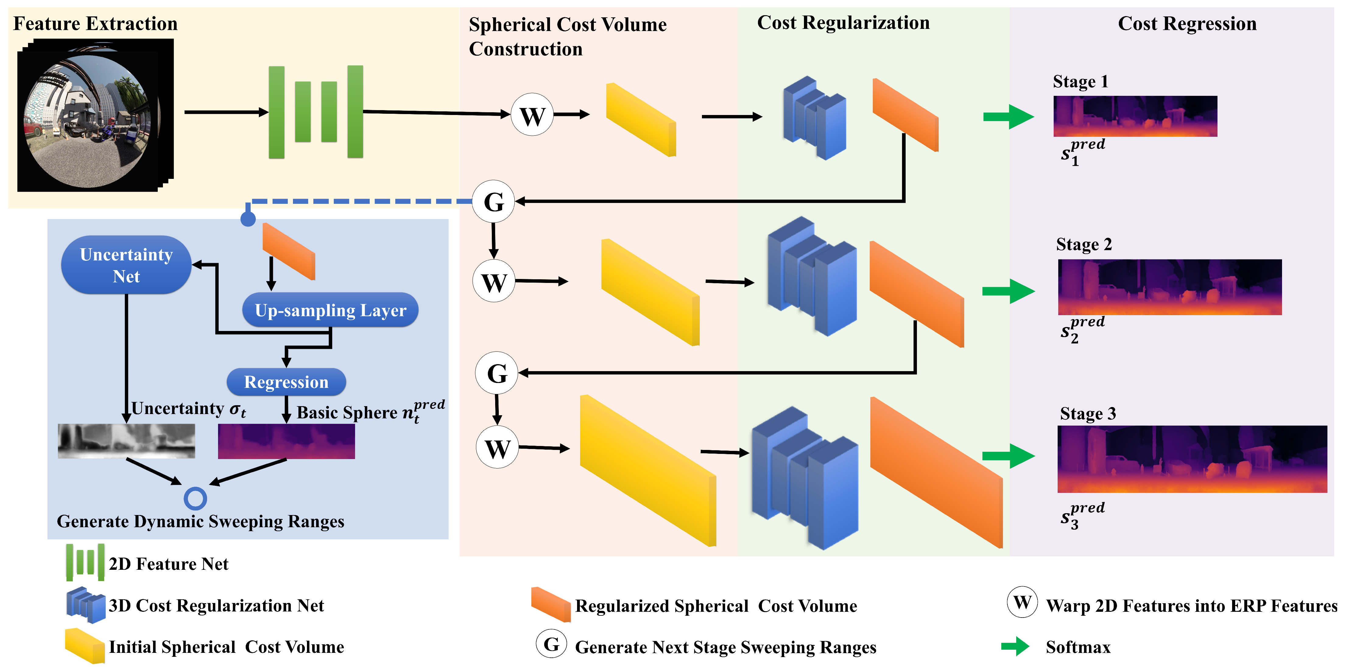
As presented in Figure 2, the proposed network consists of four parts: feature extraction, spherical cost volume construction, cost regularization, and cost regression. A three-stage cascade architecture is leveraged to construct the multi-scale spherical cost volume for a coarse-to-fine depth estimation. Furthermore, the depth range of spherical sweeping is adjusted adaptively based on the prediction and uncertainty from the previous stage.

Feature Extraction. We extract input image features using ResNet50 [30] and FPN [31], specifically the top-level FPN features with shape $\frac{1}{2}H\times \frac{1}{2}W\times C$, where H and W are input height and width.

Spherical Cost Volume Construction. The sweeping parameters in stage t are determined using Equations (10)–(13), where we project input image features onto equirectangular features based on the hypothetical spheres and camera parameters, to construct the initial spherical cost volume. As the stages progress, the resolution of equirectangular features increases, while the interval and number of hypothetical spheres decrease, as shown in

Table 1. Hyperparameter Settings. The width and height of the regularized spherical cost volume from each stage is ${\alpha }_t{H}_{output}\times {\alpha }_t{W}_{output}$.

Stage t	${\mathit{\alpha }}_{\mathit{t}}$	${\mathit{L}}_{\mathit{t}}$	${\mathit{s}}_{\mathit{t}}$	${\mathit{\lambda }}_{\mathit{t}}$	${\mathit{w}}_{\mathit{t}}$
1	0.25	48	-	4.0	0.5
2	0.50	32	3	[1.0, 4.0]	1.0
3	1.00	8	1	[1.0, 2.0]	2.0

.

Cost Regularization. We regularize the initial spherical cost volume at each stage using the cost regularization network from [11]. Each stage has a separate cost regularization network.

Cost Regression. We use soft-argmin to predict the proper sphere index $s_t^{pred}$, which is determined as

$$\begin{array}{cc}\hfill {\mathbf{p}}_t& =softmax\left(S{C}_t^{*}\right)\hfill \\ \hfill & =\left\{p_{t,min},\cdots ,p_{t,j},\cdots ,p_{t,max}\right\}\hfill \\ \hfill s_t^{pred}& =\sum _{j=S_{t,min}}^{S_{t,max}}{p}_{t,j}\ast j\hfill \end{array}$$

(1)

where $S{C}_t^{*}$ and ${\mathbf{p}}_t$ are the regularized spherical cost volume and the probability for one of the hypothetical spheres in stage t, respectively.

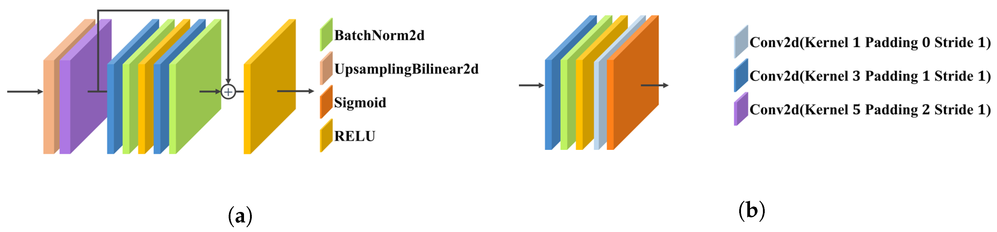
As shown in the light blue rectangular region in Figure 2, we utilize an upsampling layer (shown in Figure 3a) to increase the resolution of the regularized spherical cost volume. Then, the regression of the refined volume yields the basic sphere for sweeping, and an uncertainty net (shown in Figure 3b) is used to predict the uncertainty, thereby determining the sweeping interval and range for the next stage.

Loss Function. At each stage, all our network results are used for supervised training. The loss function uses SmoothL1Loss, which is determined as

$$loss=\sum _{t=1}^3{w}_t\times SmoothL1Loss\left(s_t^{pred},s_t^{gt}\right)$$

(2)

$s_t^{gt}$ and $w_t$ are the ground truth (GT) sphere index and the weight corresponding to the loss in stage t.

3.2. Spherical Cost Volume

Given the intrinsic and extrinsic matrices of a camera, we can project a point from the camera coordinate system to the coordinate system located at the camera rig center. Thus, we can project the feature $f_i$ from the ith camera onto the central ERP view, which can be written as

$${\mathbf{x}}_c={[x_c,y_c,z_c]}^{\mathbf{T}},$$

(3)

$$\mathbf{x}=M_{Ei}{\mathbf{x}}_c,$$

(4)

$$F_i={\mathbf{\Pi }}_i\left(M_{Ii},f_i,\mathbf{x}={\left[x,y,z\right]}^{\mathbf{T}}\right),$$

(5)

where ${\mathbf{\Pi }}_i$ is the projection function, $M_{Ii}$ and $M_{Ei}$ are the camera intrinsic and extrinsic (cam2rig) matrices, respectively, and ${\mathbf{x}}_c$ is the coordinate of point $\mathbf{P}$ in the camera coordinate system. $\mathbf{x}$ contains the 3D point coordinates in the ERP view, and $F_i$ is the ERP feature.

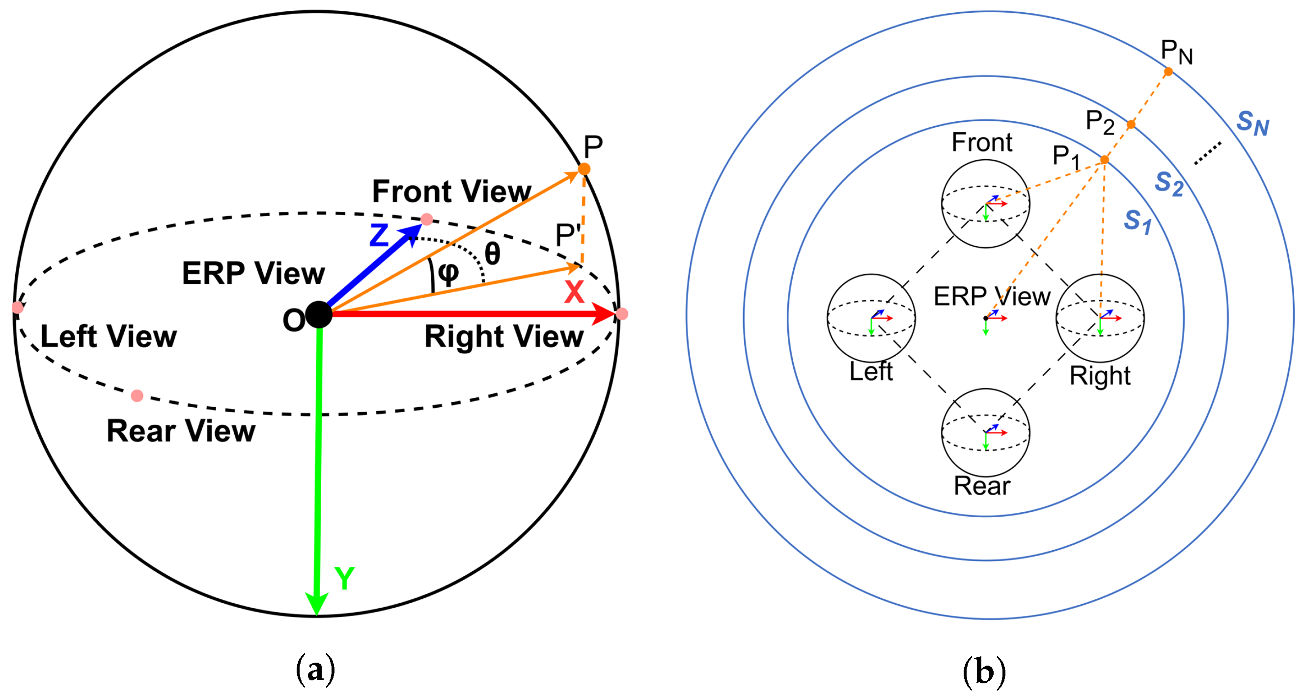
As shown in Figure 4a, we can easily transform 3D coordinates into polar coordinates. Let $\theta$ be the horizontal angle in the range $\left[-\pi ,\pi \right]$, $\varphi$ be the pitch angle in the $\left[-\frac{\pi }{2},\frac{\pi }{2}\right]$, and d be the radial distance from the point to the center. Equation (5) can be rewritten as

$$\begin{array}{cc}\hfill \theta & =arcsin\frac{x}{\sqrt{x^2+z^2}}\hfill \\ \hfill \varphi & =arctan\frac{y}{\sqrt{x^2+z^2}}\hfill \\ \hfill d& =\sqrt{x^2+y^2+z^2}\hfill \\ \hfill F_i& ={\mathbf{\Pi }}_i\left(M_{Ii},f_i,\left(\theta ,\varphi ,d\right)\right)\hfill \end{array}$$

(6)

The values of $\theta$ and $\varphi$ can be readily derived from ERP images. Consequently, a backward warp can be performed using $\theta$, $\varphi$, and d to obtain the ERP feature. Varying d yields different projection outcomes, enabling computation of the spherical cost volume. We divide the inverse of the depth into a finite number of hypothetical spheres, which is determined as

$$idx=\frac{N-1}{d_{max}^{{}^{\prime }}-d_{min}^{{}^{\prime }}}\left(d^{{}^{\prime }}-d_{min}^{{}^{\prime }}\right),$$

(7)

where N is the total number of hypothetical spheres, $d^{{}^{\prime }}$ is the inverse depth $\frac{1}{d}$, $d_{max}^{{}^{\prime }},d_{min}^{{}^{\prime }}$ are the maximum and minimum values, respectively, and $idx$ represents the index of the hypothetical sphere $S_{idx+1}$.

As shown in Figure 4b, given a series of hypothetical spheres $\left\{S_1,S_2,\cdots ,S_j,\cdots ,S_L\right\}$, we can obtain the ERP features at each index based on Equations (4), (6) and (7). By concatenating these features together, we form the spherical feature volume for the $i^{th}$ camera, which is denoted as

$$S{C}_i=concatenate\left\{F_{i,1},\cdots ,F_{i,j},\cdots ,F_{i,L}\right\},$$

(8)

where $S{C}_i$ is the spherical feature volume, and $F_{i,j}$ is the feature of the hypothetical sphere $S_j$. If the shape of $F_{i,j}$ is $H^{{}^{\prime }}\times W^{{}^{\prime }}\times C$, then the shape of $S{C}_i$ is $H^{{}^{\prime }}\times W^{{}^{\prime }}\times C\times L$, where $H^{{}^{\prime }}$, $W^{{}^{\prime }}$, and C represent the height, width, and number of channels, respectively.

We can calculate the variance between the spherical feature volumes of different cameras and take this as the initial spherical cost volume $SC$ in the ERP view, which is determined as

$$SC=\frac{{\sum }_{i=1}^{m}S{C}_i^2}{m}-{\left(\frac{{\sum }_{i=1}^{m}S{C}_i}{m}\right)}^2,$$

(9)

where m is the number of cameras. By performing cost regularization and regression, the initial spherical cost volume enables identifying the proper sphere and corresponding depth for each 3D point.

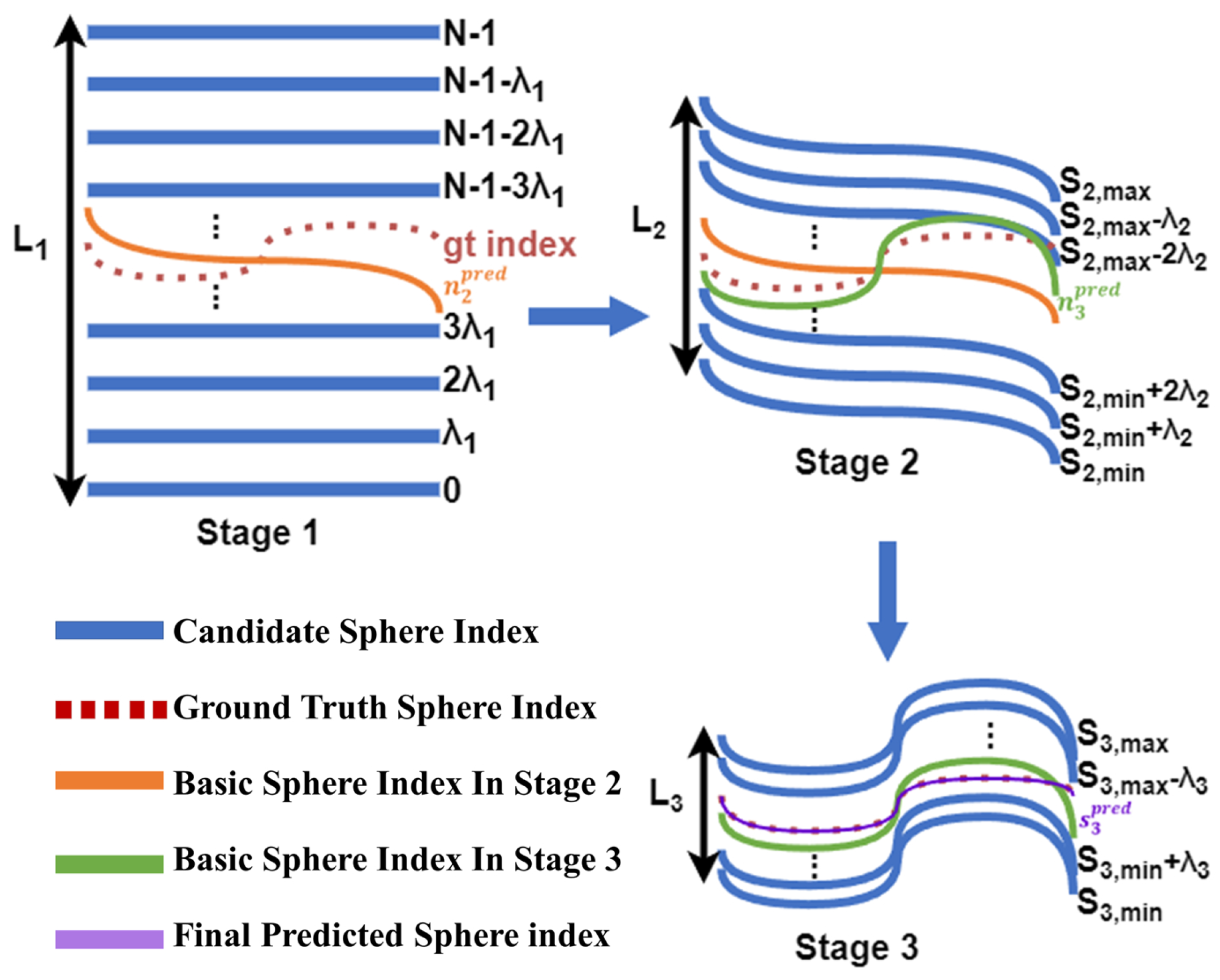
3.3. Cascade Spherical Sweeping

We propose a cascade spherical sweeping approach, enabling high accuracy, while reducing resource use. The initial stage using the low-resolution spherical cost volume sweeps more hypothetical spheres for a coarse estimate. Based on this estimation, in the high-resolution space, we perform spherical sweeping with fewer but more accurate hypothetical spheres, leading to better results.

As shown in Figure 5, the proposed cascade spherical sweeping consists of three stages. Let $L_t$ represent the number of hypothetical spheres in stage t. The shape of the corresponding initial spherical cost volume is $H_t\times W_t\times C\times L_t$, with the sweeping interval ${\lambda }_t$. $h_t$ is a parameter defined by Equation (12), which is used to determine the sweeping range. In stage 1, we construct the spherical cost volume over the entire hypothetical spherical space at a low resolution, where ${\lambda }_1=\frac{N}{L_1}$. In the subsequent stages, each stage utilizes the outcome of the previous one as the basic sphere $n_t^{pred}$ to initiate sweeping, with the range determined by applying offsets based on $h_t$, which is determined as

$$S_{t,min}=\left\{\begin{array}{cc}0\hfill & \mathrm{if}{n}_t^{pred}-h_t\frac{L_t}{2}<0\hfill \\ N-h_t{L}_t\hfill & \mathrm{if}{n}_t^{pred}+h_t\frac{L_t}{2}\ge N\hfill \\ n_t^{pred}-h_t\frac{L_t}{2}\hfill & \mathrm{otherwise}\hfill \end{array}\right.,$$

(10)

$$S_{t,max}=\left\{\begin{array}{cc}{h}_t{L}_t-1\hfill & \mathrm{if}{n}_t^{pred}-h_t\frac{L_t}{2}<0\hfill \\ N-1\hfill & \mathrm{if}{n}_t^{pred}+h_t\frac{L_t}{2}\ge N\hfill \\ n_t^{pred}+h_t\frac{L_t}{2}\hfill & \mathrm{otherwise}\hfill \end{array}\right.,$$

(11)

where $S_{t,min}$ and $S_{t,max}$ denote the lower and upper limits of the sweeping range in stage t, respectively. $n_t^{pred}$ is obtained using Equation (1) but using the upsampled $S{C}_t^{*}$.

3.4. Dynamic Sweeping Range with Uncertainty

In stages 2 and 3, we upsample the regularized cost volumes and use them to obtain the sweeping interval and range based on Equations (10) and (11). The interval is computed as

$$h_t=1.0+s_t\times {\sigma }_t,$$

(12)

$${\lambda }_t=\frac{\left(S_{t,max}-S_{t,min}+1\right)}{L_t},$$

(13)

where $s_t$ is a hyperparameter in stage t, serving to restrict the range of the interval, and ${\sigma }_t\in [0,1]$ is the uncertainty predicted by a dedicated subnetwork (called uncertainty net). If the uncertainty of a pixel is high, the range of spherical sweeping performed at that point will also expand to find the best matching sphere.

The uncertainty signifies the deviation between the predicted and ground truth spheres. High uncertainty requires expanding the sweeping range due to the large bias. In contrast, low uncertainty allows narrowing the range as the result approaches the true value. Our method adaptively adjusts the sweeping range and interval based on a per-pixel point uncertainty to dynamically determine a reasonable scope. This method searches for a sphere within the hypothetical region where each pixel is most likely to be located.

4. Experiments

4.1. Implementation Details

We trained the full network end-to-end using an Adam optimizer on 8 RTX3090 GPUs, with a batch size of 2 per GPU. We set $N=192$ and $C=32$, with $d_{min}^{{}^{\prime }}=\frac{1}{1000m}$ and $d_{max}^{{}^{\prime }}=\frac{1}{1.65m}$. In all experiments, the output and GT depth maps were cropped to $H_{output}=160$ ($\frac{-\pi }{4}\le \varphi \le \frac{\pi }{4}$) and $W_{output}=640$ to exclude regions near the poles that were highly distorted and less informative. The hyperparameter details mentioned in Section 3 are described in Table 1.

We trained on OmniThings for 30 epochs with an initial learning rate $l=0.001$, decayed by a cosine scheduler after 6 warm up epochs. We then fine-tuned on Urban and OmniHouse for 20 epochs, with $l=0.001$ for the first 10 epochs and $l=0.0001$ after.

4.2. Quantitative Evaluation

To evaluate our method, we conducted a comparative analysis with several publicly available methods. The resource usage of the different models during the inference process and the datasets used for training are summarized in

Table 2. Summary of model information. ‘-ft’ represents the fine-tuned model. The best results are in bold. ‘✓’ indicates that the dataset is used for training.

Models	GPU Memory Utilization (MiB)	Inference Time (Seconds)	Training Data
			OmniThings [8]	OmniHouse [8]	Urban [8]
Crown360 [27]	3772	∼0.231	✓
OmniMVS-ft [8]	7720	∼0.320	✓	✓	✓
CasOmniMVS (ours)	3022	∼0.085	✓
CasOmniMVS-ft (ours)	3022	∼0.085	✓	✓	✓

. The results clearly demonstrate that our method exhibited the lowest GPU memory utilization and the fastest inference time. All models used training weights provided by the authors.

For quantitative evaluation, we calculated the error by converting the predicted sphere indices into absolute depth values using Equation (7). We used metrics such as MAE (mean absolute error), RMSE (root mean square error), AbsRel (absolute relative error), and SqRel (squared relative error), as presented in

Table 3. Quantitative results (depth) on the synthetic datasets. The metrics refer to depth errors. The best results are in bold. ‘↓’ indicates that the smaller the value, the better.

Datasets	Methods	Metrics
		MAE (↓)	RMSE (↓)	AbsRel (↓)	SqRel (↓)
OmniThings	Crown360 [27]	1.788	5.307	0.161	5.554
	OmniMVS-ft [8]	2.363	7.883	0.283	15.169
	CasOmniMVS	0.604	1.420	0.045	0.227
	CasOmniMVS-ft	0.949	2.018	0.060	0.454
OmniHouse	Crown360 [27]	1.694	4.141	0.102	1.535
	OmniMVS-ft [8]	0.631	2.292	0.044	0.582
	CasOmniMVS	0.807	1.889	0.049	0.222
	CasOmniMVS-ft	0.497	1.321	0.029	0.118
Sunny	Crown360 [27]	4.244	10.707	0.180	5.091
	OmniMVS-ft [8]	1.772	6.979	0.083	2.807
	CasOmniMVS	2.750	8.042	0.119	2.577
	CasOmniMVS-ft	1.471	5.736	0.051	1.162

. As shown in

Table 4. Quantitative results (index) on the synthetic datasets. The qualifier ‘>n’ refers to the pixel ratio (%) whose error is larger than n. The best results are in bold. ‘↓’ indicates that the smaller the value, the better.

Datasets	Methods	Metrics
		MAE (↓)	RMSE (↓)	>1 (↓)	>3 (↓)	>5 (↓)
OmniThings	Crown360 [27]	2.566	4.900	48.051	21.648	13.410
	OmniMVS-ft [8]	3.330	6.949	43.811	24.603	17.512
	CasOmniMVS	1.156	3.016	23.355	7.664	4.363
	CasOmniMVS-ft	1.516	3.610	31.262	11.309	6.373
OmniHouse	Crown360 [27]	1.399	2.921	29.947	8.905	5.036
	OmniMVS-ft [8]	0.618	1.626	9.698	3.436	2.055
	CasOmniMVS	0.793	1.777	15.178	4.490	2.321
	CasOmniMVS-ft	0.451	1.075	7.164	1.841	1.029
Sunny	Crown360 [27]	1.352	2.896	33.407	9.253	4.971
	OmniMVS-ft [8]	0.597	2.453	7.766	3.700	2.504
	CasOmniMVS	1.216	3.205	23.269	8.469	4.808
	CasOmniMVS-ft	0.446	1.570	6.807	2.191	1.277

, the error was also measured using the percent error [8] of the estimated sphere index compared to all possible spheres, which is defined as

$$Erro{r}_{index}=\frac{\left|s_3^{pred}-s_3^{gt}\right|}{N}\times 100,$$

(14)

The quantitative results demonstrated that our method achieved the best performance compared to the other methods. The depth range for the evaluation metric was [1.65 m, 100 m]. As shown in Table 2, we also evaluated the GPU memory usage and inference speed, and the results showed that our method was more efficient.

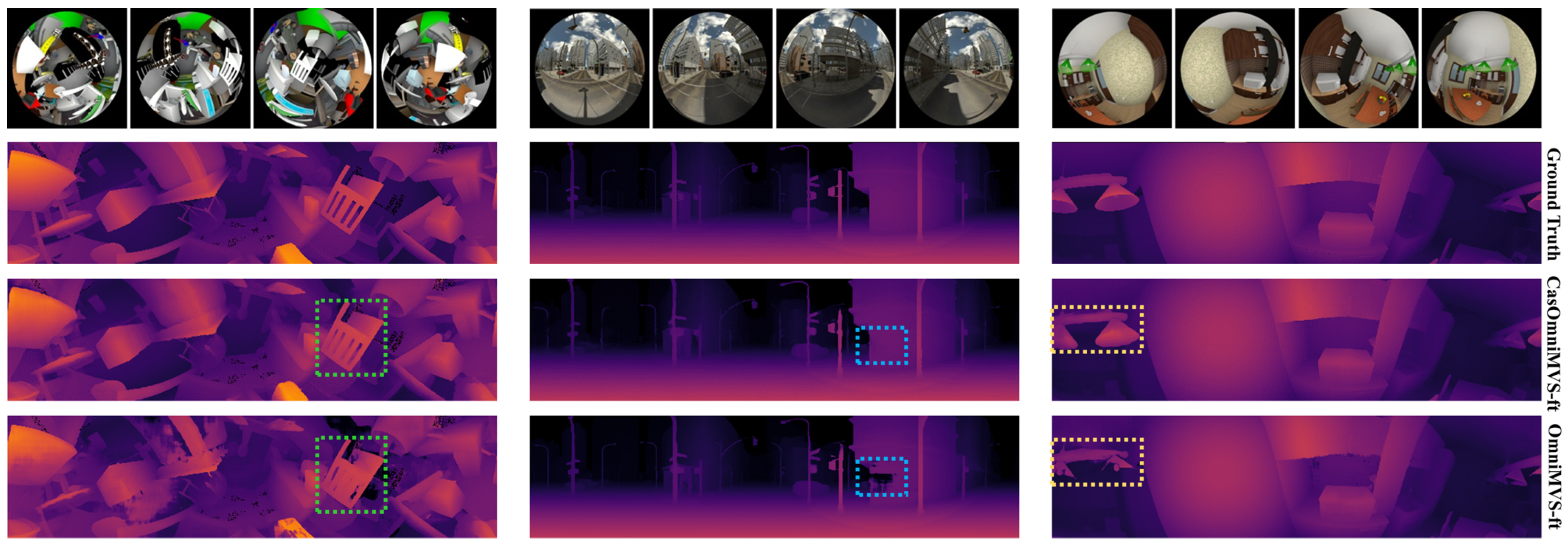
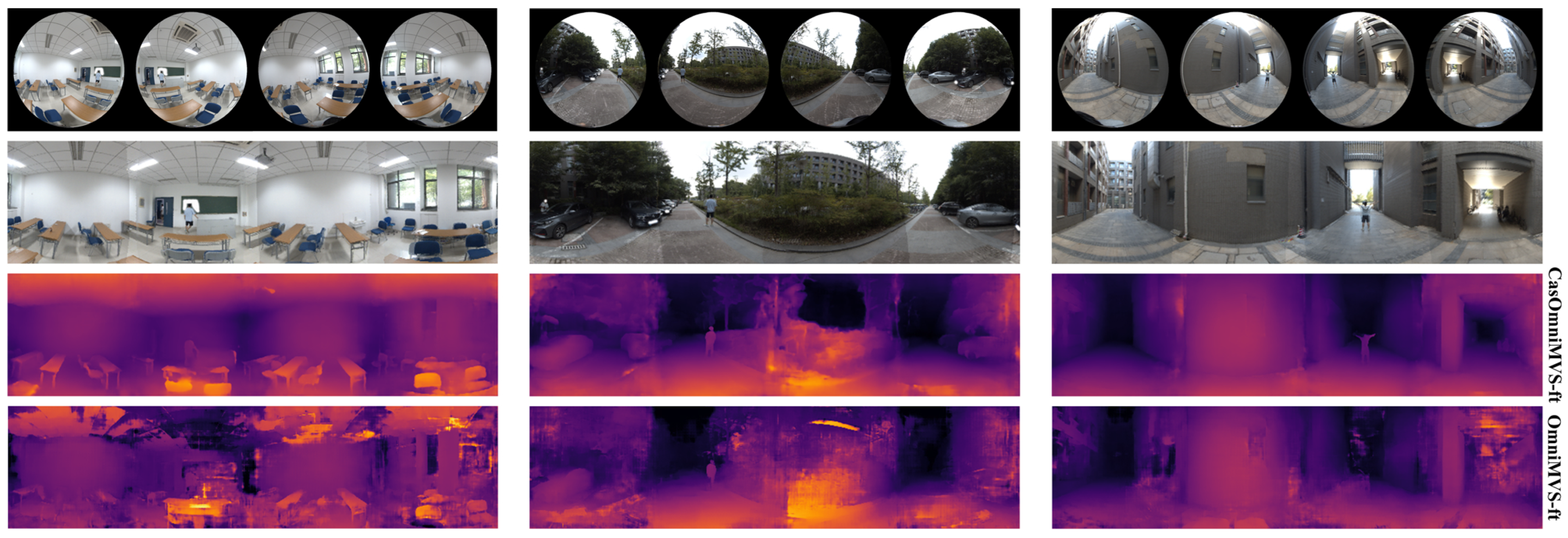
4.3. Qualitative Evaluation

Figure 6 illustrates the qualitative results of our and other methods on the synthetic datasets. Our method outperformed the other methods in areas such as detail (the area surrounded by the short green line), glass reflections (the area surrounded by the short blue lines), and translucent material objects (the area surrounded by the short yellow lines). Furthermore, as illustrated in Figure 7, our model achieved impressive results even in real-world scenarios, despite only being trained on synthetic data.

4.4. Ablation Studies

Evaluation of Dynamic Spherical Sweeping. We compared the performance of the proposed method with and without dynamic spherical sweeping (dss). VAR represents using the variance used in [10,18] to estimate the uncertainty ${\sigma }_t$. All networks had data augmentation disabled during training.

Table 5. Quantitative results (index) on the omnithings dataset with dynamic spherical sweeping. The best results are in bold. ‘↓’ indicates that the smaller the value, the better.

Network Setting	MAE (↓)	RMSE (↓)	>1 (↓)	>3 (↓)	>5 (↓)
w/o dss	1.1803	3.3381	20.7600	7.8810	4.6502
w/dss(VAR)	1.2627	3.1713	25.6427	9.3490	5.1254
w/dss	1.0676	2.9761	20.2148	6.8897	3.8971

shows the ablation studies of the proposed dynamic spherical sweeping. For the non-dynamic spherical sweeping method, $h_2$ and $h_3$ were set to 2.0 and 1.0, respectively. The variance was defined as

$$va{r}_t=\sum _{j=S_{t,min}}^{S_{t,max}}{(s_t^{pred}-j)}^2\times p_{t,j},$$

(15)

where $va{r}_t$ is the variance in stage t. The results demonstrated the superiority of our method over the fixed-interval and variance-based uncertainty prediction approaches.

Evaluation of Cascade Strategy. We used the fine-tuned model to test the results of different stages and conducted a quantitative comparison, as shown in

Table 6. Quantitative results(index) of different stages. The error was measured using Equation (14). ‘↓’ indicates that the smaller the value, the better.

Datasets	Stage t	MAE (↓)	RMSE (↓)	>1 (↓)	>3 (↓)	>5 (↓)
OmniThings	1	2.5987	5.4940	47.6431	19.3850	12.1928
	2	1.8062	4.2154	35.5856	13.0703	7.8032
	3	1.5157	3.6077	31.2624	11.3088	6.3731
OmniHouse	1	0.7597	1.7285	15.4238	3.3810	1.8910
	2	0.5407	1.3086	8.7325	2.2392	1.2954
	3	0.4508	1.0750	7.1639	1.8408	1.0288
Sunny	1	1.1544	2.7189	32.8847	4.9705	3.2113
	2	0.6490	1.9355	9.4358	2.9383	1.8798
	3	0.4459	1.5696	6.8069	2.1911	1.2773

. The results demonstrated that our cascade strategy could progressively improve the prediction accuracy. Figure 8 illustrates that the network predictions were continuously refined from coarse to fine as the stages advanced.

5. Conclusions, Limitations, and Future Work

In this work, we proposed an end-to-end cascade omnidirectional depth estimation algorithm with dynamic spherical sweeping. It begins with a low-resolution spherical cost volume, then progressively refines the resolution, while adaptively adjusting sweeping intervals and ranges. The experimental results demonstrated that our method significantly reduced the GPU memory usage and sped up the inference time, outperforming various existing publicly available omnidirectional depth estimation algorithms. Furthermore, without fine-tuning, our method also produced promising results in real-world scenarios, showing a high generalizability and practicality.

Our method relies on the feature matching in the overlapping regions between camera views, leading to a less accurate performance in non-overlapping regions. When constructing the spherical cost volume, we simply calculated the variance between multi-view features, without explicitly differentiating overlapping and non-overlapping regions. In future work, we will focus on how to effectively leverage features from overlapping versus non-overlapping areas, to optimize cost volume generation. Furthermore, optimizing the division of hypothetical spheres based on the different depth distribution of various scenes (i.e. indoor and outdoor) is also an exciting research direction. We will also explore the application of self-supervised learning, to improve our method.

References

- Zioulis, N.; Karakottas, A.; Zarpalas, D.; Daras, P. OmniDepth: Dense Depth Estimation for Indoors Spherical Panoramas. In Proceedings of the European Conference on Computer Vision (ECCV), Munich, Germany, 8–14 September 2018; pp. 453–471. [Google Scholar]
- Li, Y.; Yan, Z.; Duan, Y.; Ren, L. PanoDepth: A Two-Stage Approach for Monocular Omnidirectional Depth Estimation. arXiv 2022, arXiv:2202.01323. [Google Scholar]
- Li, Y.; Guo, Y.; Yan, Z.; Huang, X.; Ye, D.; Ren, L. OmniFusion: 360 Monocular Depth Estimation via Geometry-Aware Fusion. In Proceedings of the 2022 Conference on Computer Vision and Pattern Recognition (CVPR), New Orleans, LO, USA, 19–24 June 2022. [Google Scholar]
- Jiang, H.; Sheng, Z.; Zhu, S.; Dong, Z.; Huang, R. UniFuse: Unidirectional Fusion for 360° Panorama Depth Estimation. IEEE Robot. Autom. Lett. 2021, 6, 1519–1526. [Google Scholar] [CrossRef]
- Zioulis, N.; Karakottas, A.; Zarpalas, D.; Alvarez, F.; Daras, P. Spherical View Synthesis for Self-Supervised 360 Depth Estimation. arXiv 2019, arXiv:1909.08112. [Google Scholar]
- Wang, N.H.; Solarte, B.; Tsai, Y.H.; Chiu, W.C.; Sun, M. 360SD-Net: 360∘ Stereo Depth Estimation with Learnable Cost Volume. In Proceedings of the 2020 IEEE International Conference on Robotics and Automation (ICRA), Virtual, 31 May–15 June 2020; pp. 582–588. [Google Scholar] [CrossRef]
- Li, M.; Jin, X.; Hu, X.; Dai, J.; Du, S.; Li, Y. MODE: Multi-view Omnidirectional Depth Estimation with 360∘ Cameras. In Proceedings of the Computer Vision—ECCV 2022, Tel Aviv, Israel, 23–24 October 2022; pp. 197–213. [Google Scholar]
- Won, C.; Ryu, J.; Lim, J. End-to-end learning for omnidirectional stereo matching with uncertainty prior. IEEE Trans. Pattern Anal. Mach. Intell. 2020, 43, 3850–3862. [Google Scholar] [CrossRef] [PubMed]
- Won, C.; Ryu, J.; Lim, J. SweepNet: Wide-baseline Omnidirectional Depth Estimation. In Proceedings of the 2019 International Conference on Robotics and Automation (ICRA), Montreal, QC, Canada, 20–24 May 2019; pp. 6073–6079. [Google Scholar] [CrossRef]
- Cheng, S.; Xu, Z.; Zhu, S.; Li, Z.; Li, L.E.; Ramamoorthi, R.; Su, H. Deep Stereo Using Adaptive Thin Volume Representation With Uncertainty Awareness. In Proceedings of the 2020 IEEE/CVF Conference on Computer Vision and Pattern Recognition (CVPR), Seattle, WA, USA, 13–19 June 2020; pp. 2521–2531. [Google Scholar] [CrossRef]
- Gu, X.; Fan, Z.; Zhu, S.; Dai, Z.; Tan, F.; Tan, P. Cascade Cost Volume for High-Resolution Multi-View Stereo and Stereo Matching. In Proceedings of the 2020 IEEE/CVF Conference on Computer Vision and Pattern Recognition, CVPR 2020, Seattle, WA, USA, 13–19 June 2020; pp. 2492–2501. [Google Scholar] [CrossRef]
- Žbontar, J.; LeCun, Y. Stereo Matching by Training a Convolutional Neural Network to Compare Image Patches. J. Mach. Learn. Res. 2016, 17, 1–32. [Google Scholar]
- Hirschmuller, H. Accurate and efficient stereo processing by semi-global matching and mutual information. In Proceedings of the 2005 IEEE Computer Society Conference on Computer Vision and Pattern Recognition (CVPR’05), San Diego, CA, USA, 2–6 October 2005; Volume 2, pp. 807–814. [Google Scholar] [CrossRef]
- Kendall, A.; Martirosyan, H.; Dasgupta, S.; Henry, P.; Kennedy, R.; Bachrach, A.; Bry, A. End-to-End Learning of Geometry and Context for Deep Stereo Regression. In Proceedings of the 2017 IEEE International Conference on Computer Vision (ICCV), Venice, Italy, 22–29 October 2017; pp. 66–75. [Google Scholar] [CrossRef]
- Chang, J.; Chen, Y. Pyramid Stereo Matching Network. In Proceedings of the 2018 IEEE/CVF Conference on Computer Vision and Pattern Recognition, Salt Lake City, UT, USA, 18–23 June 2018; pp. 5410–5418. [Google Scholar] [CrossRef]
- Zhang, F.; Prisacariu, V.; Yang, R.; Torr, P.H. GA-Net: Guided Aggregation Net for End-to-end Stereo Matching. In Proceedings of the IEEE Conference on Computer Vision and Pattern Recognition, Long Beach, CA, USA, 16–17 June 2019; pp. 185–194. [Google Scholar]
- Lipson, L.; Teed, Z.; Deng, J. RAFT-Stereo: Multilevel Recurrent Field Transforms for Stereo Matching. In Proceedings of the International Conference on 3D Vision (3DV), Virtual, 1–3 December 2021. [Google Scholar]
- Shen, Z.; Dai, Y.; Rao, Z. CFNet: Cascade and Fused Cost Volume for Robust Stereo Matching. In Proceedings of the IEEE Conference on Computer Vision and Pattern Recognition, CVPR 2021, Virtual, 19–25 June 2021; pp. 13906–13915. [Google Scholar] [CrossRef]
- Yao, Y.; Luo, Z.; Li, S.; Fang, T.; Quan, L. MVSNet: Depth inference for unstructured multi-view stereo. In Proceedings of the European Conference on Computer Vision (ECCV), Munich, Germany, 8–14 September 2018; pp. 767–783. [Google Scholar]
- Yao, Y.; Luo, Z.; Li, S.; Shen, T.; Fang, T.; Quan, L. Recurrent MVSNet for High-Resolution Multi-View Stereo Depth Inference. In Proceedings of the IEEE Conference on Computer Vision and Pattern Recognition, CVPR 2019, Long Beach, CA, USA, 16–20 June 2019; pp. 5525–5534. [Google Scholar] [CrossRef]
- Chen, R.; Han, S.; Xu, J.; Su, H. Point-Based Multi-View Stereo Network. In Proceedings of the 2019 IEEE/CVF International Conference on Computer Vision (ICCV), Seoul, Republic of Korea, 27 October–2 November 2019; pp. 1538–1547. [Google Scholar] [CrossRef]
- Xue, Y.; Chen, J.; Wan, W.; Huang, Y.; Yu, C.; Li, T.; Bao, J. MVSCRF: Learning Multi-View Stereo with Conditional Random Fields. In Proceedings of the 2019 IEEE/CVF International Conference on Computer Vision (ICCV), Seoul, Republic of Korea, 27 October–2 November 2019; pp. 4311–4320. [Google Scholar] [CrossRef]
- Wikipedia, The Free Encyclopedia. Equirectangular Projection. 2023. Available online: https://en.wikipedia.org/w/index.php?title=Equirectangular_projection&oldid=1168045951 (accessed on 7 August 2023).
- Wang, F.E.; Yeh, Y.H.; Sun, M.; Chiu, W.C.; Tsai, Y.H. BiFuse: Monocular 360 Depth Estimation via Bi-Projection Fusion. In Proceedings of the 2020 IEEE/CVF Conference on Computer Vision and Pattern Recognition (CVPR), Seattle, WA, USA, 14–19 June 2020; pp. 459–468. [Google Scholar] [CrossRef]
- Li, M.; Hu, X.; Dai, J.; Li, Y.; Du, S. Omnidirectional stereo depth estimation based on spherical deep network. Image Vis. Comput. 2021, 114, 104264. [Google Scholar] [CrossRef]
- Wikipedia, The Free Encyclopedia Cassini Projection. Available online: https://en.wikipedia.org/w/index.php?title=Cassini_projection&oldid=1132701624 (accessed on 22 July 2023).
- Komatsu, R.; Fujii, H.; Tamura, Y.; Yamashita, A.; Asama, H. 360° Depth Estimation from Multiple Fisheye Images with Origami Crown Representation of Icosahedron. In Proceedings of the 2020 IEEE/RSJ International Conference on Intelligent Robots and Systems (IROS), Las Vegas, NV, USA, 25–29 October 2020; pp. 10092–10099. [Google Scholar] [CrossRef]
- Chen, Z.; Lin, C.; Nie, L.; Liao, K.; Zhao, Y. Unsupervised OmniMVS: Efficient Omnidirectional Depth Inference via Establishing Pseudo-Stereo Supervision. arXiv 2023, arXiv:2302.09922. [Google Scholar]
- Xie, S.; Wang, D.; Liu, Y.H. OmniVidar: Omnidirectional Depth Estimation From Multi-Fisheye Images. In Proceedings of the IEEE/CVF Conference on Computer Vision and Pattern Recognition (CVPR), Vancouver, BC, Canada, 18–22 June 2023; pp. 21529–21538. [Google Scholar]
- He, K.; Zhang, X.; Ren, S.; Sun, J. Deep Residual Learning for Image Recognition. In Proceedings of the 2016 IEEE Conference on Computer Vision and Pattern Recognition (CVPR), Las Vegas, NV, USA, 27–30 June 2016; pp. 770–778. [Google Scholar] [CrossRef]
- Lin, T.Y.; Dollár, P.; Girshick, R.; He, K.; Hariharan, B.; Belongie, S. Feature Pyramid Networks for Object Detection. In Proceedings of the 2017 IEEE Conference on Computer Vision and Pattern Recognition (CVPR), Honolulu, HI, USA, 21–26 July 2017; pp. 936–944. [Google Scholar] [CrossRef]
Figure 1.
Omnidirectional depth estimation. (Left Top): The structure of the system with fisheye images as input. (Left Bottom): Real camera rig. (Right Top): Panoramic image. (Right Middle): Panoramic inverse depth map. (Right Bottom): Point cloud image.
Figure 2.
Network architecture overview. Our network is roughly divided into four parts: feature extraction, spherical cost volume construction, cost regularization, and cost regression.
Figure 3.
Network submodules. Each stage has its own independent uncertainty net and upsampling layer. (a) Upsampling layer; (b) uncertainty net.
Figure 4.
(a) Illustration of the coordinate system. The color arrows indicate the three axes of the 3D Cartesian coordinate system. The point can be projected into the ERP view with the camera rig center as the origin. is the projection point of on the plane. is the angle between and . is the angle between and . (b) Illustration of multi-view spherical sweeping. We can assume that is in different hypothetical spheres to construct a spherical cost volume.
Figure 5.
Cascade spherical sweeping in different stages. In the three stages, our method’s prediction becomes closer to the ground truth.
Figure 6.
Qualitative results on the synthetic datasets. Visualizing the inverse of the depth, with a minimum depth of 1.65 m.
Figure 7.
Qualitative results on the real data. Visualizing the inverse of the depth, with a minimum depth of 1.25 m.
Figure 8.
Qualitative results (index) of multiple cascade stages. For each image group, from left to right, the first row displays the input image, ground truth, and colors corresponding to the different sphere indices. The second row shows the visualization of sphere indices (maximum sphere indices were set to 95 and 125, respectively), and the third row presents the error maps (maximum sphere index error was set to 5) for the three stages.