Abstract
Non-intrusive load monitoring (NILM) technology, crucial for intelligent electricity management, has gained considerable attention in residential electricity usage studies. NILM enables monitoring of total electrical current and voltage in homes, offering insights vital for enhancing safety and preventing domestic electrical accidents. Despite its importance, accurately discerning the operational status of appliances using non-intrusive methods remains a challenging area within this field. This paper presents a novel methodology that integrates an advanced clustering algorithm with a Bayesian network for the identification of appliance operational states. The approach involves capturing the electrical current signals during appliance operation via NILM, followed by their decomposition into odd harmonics. An enhanced clustering algorithm is then employed to ascertain the central coordinates of the signal clusters. Building upon this, a three-layer Bayesian network inference model, incorporating leak nodes, is developed. Within this model, harmonic signals are used as conditions for node activation. The operational states of the appliances are subsequently determined through probabilistic reasoning. The proposed method’s effectiveness is validated through a series of simulation experiments conducted in a laboratory environment. The results of these experiments (low mode 89.1%, medium mode 94.4%, high mode 92.0%, and 98.4% for combination) provide strong evidence of the method’s accuracy in inferring the operational status of household electrical appliances based on NILM technology.
1. Introduction
The analysis of electrical behavior is a critical aspect of electric energy research, particularly in the context of the rapidly evolving smart grid technology. This analysis plays a pivotal role in effectively evaluating current power consumption within power networks and facilitating power quality monitoring. By implementing effective monitoring and analysis of electricity consumption, it is possible to ensure the safety of electricity usage, prevent electrical equipment failures, and comprehend users’ electricity consumption behaviors. These insights are instrumental in formulating scientific and reasonable electricity consumption strategies, thereby ensuring the supply of high-quality electric energy and minimizing energy waste, which are crucial for environmental protection.
The intertwining of global economic development with energy consumption, particularly with the uptake of electric vehicles, is evident in the rising use of electricity across various sectors. According to data from the U.S. Energy Information Administration, the electricity end-use in 2022 for residential, commercial, and industrial sectors was 1,521,886, 1,373,031, and 1,007,533 million kilowatt-hours, respectively [1]. This underscores the critical need for effective power energy management and strategic power supply planning, which are vital for national progress and public welfare. Advancements in power quality monitoring research are essential for discerning consumption patterns and devising suitable supply strategies.
Electricity network analysis leverages two main approaches: intrusive load monitoring (ILM) and non-intrusive load monitoring (NILM) [2]. ILM connects directly to appliances to gather precise data, offering detailed insights at a higher cost and invasiveness. NILM, in contrast, assesses overall consumption from a single point, distinguishing individual appliances through algorithmic estimations. It is recognized for its cost-efficiency and minimally invasive setup [3]. NILM has surged ahead, favored for its non-disruptive nature, straightforward data collection, and low overheads. As the preferred method for electrical behavior analysis, NILM’s various strategies have been comprehensively cataloged by Aladesanmi and Folly [4].
Current NILM-related research primarily focuses on identifying household electrical equipment due to NILM technology’s unique characteristics. With each type of equipment exhibiting distinct electrical behavior characteristics during operation, numerous researchers are exploring NILM methods for device recognition based on these traits. The classification of household electrical equipment types or working modes is fundamental to this identification process. Sultanem initially proposed a classification system for household electrical equipment, categorized as follows [5]:
- Resistive appliances: heating devices and similar equipment characterized by zero reactive power, no transient during activation, and the absence of harmonics.
- Pump-operated appliances: motor-driven, with substantial reactive power.
- Motor-driven appliances: examples include washing machines and fans, exhibiting less substantial activation transients.
- Electronically fed appliances: characterized by short but high-amplitude activation transients.
- Electronic power control appliances.
- Fluorescent lighting.
In the realm of NILM technology for identifying electrical equipment, diverse parameter signals are utilized as the basis for analysis. These include power signatures with consistent real and reactive power [6,7,8,9,10], voltage and current trajectories [11,12], and harmonic analysis [13,14,15,16]. Each of these studies significantly contributes to the performance of various analysis methods. Recent advancements in NILM have significantly contributed to the field of energy management, offering innovative solutions for disaggregating total energy consumption into appliance-level usage, focusing on adaptive modeling, machine learning algorithms, and integration with IoT for both residential and industrial applications.
In the realm of adaptive modeling and machine learning for non-intrusive load monitoring (NILM), significant strides have been made by researchers like Wang et al. [17] and Grover et al. [18]. Their pioneering work in employing convolutional neural networks (CNNs) and adaptive models addresses the dynamic nature of electrical loads and grid conditions, a critical aspect in the evolution of NILM technologies. Green and Garimella [19] applied supervised graph signal processing for residential load disaggregation, emphasizing the importance of NILM in demand-side management. Focusing on the challenge of appliance identification and load disaggregation, studies by Aslan and Zurel [20], Nie et al. [21], and Qu et al. [22] underscored the critical role of accurate appliance recognition in enhancing the efficiency and reliability of NILM systems, utilizing time series analysis and deep feature-guided mechanisms. Addressing the practical challenges and opportunities in real-world NILM applications, Yan et al. [23] provided an insightful overview, particularly emphasizing the potential of machine learning in overcoming these obstacles. In the integration of IoT and multimodal data into NILM, Ghosh et al. [24] and Keramati et al. [25] showcased the potential of technology-enhanced systems in smart energy management, marking a significant advancement in the field. In industrial and complex environments, the works of Luan et al. [26], Li et al. [27], and Cui et al. [28] highlight the complexity and necessity of tailored NILM solutions in energy-intensive industrial settings, addressing the unique challenges of industrial load disaggregation.
Recent NILM research has advanced towards adaptive and intelligent energy management systems, integrating machine learning [29] and IoT technologies [30] to enhance system accuracy and expand use in residential and industrial settings. Methods like electrical quantities [31,32,33], power theories [34,35,36], and harmonic decomposition [37,38] are widely used. This paves the way for more sustainable energy use. However, existing methods focusing on current, voltage, and power analysis are limited and not fully representative. Traditional threshold-based load identification methods, although straightforward, face challenges in typical households due to the difficulty in collecting device data and high false-positive rates for new or similar devices.
In addressing these challenges, a novel power load identification method is proposed that integrates clustering algorithms with probabilistic graph models. This method begins with the acquisition of electrical behavior characteristics of equipment via NILM, followed by load decomposition to obtain electrical signal parameters under operational states. Subsequently, an electrical behavior event division method is employed to categorize the collected electrical signal parameters into events, identifying independent parameter events within each signal. An improved K-means method is then utilized to cluster the power consumption behavior characteristics under various parameters, determining the feature center. Building upon this, a Bayesian network model is established, including Noisy-Max nodes and leak nodes, with distinct node characteristics set to facilitate the identification of electrical equipment operating states through probabilistic reasoning. A two-layer identification model is thus formulated. The upper layer represents the operating states of the equipment, with each node signifying a specific load equipment state. The lower layer comprises cluster nodes, each denoting the center of a cluster. The proximity of data to the cluster center determines its contribution rate to the cluster, which can be translated into probabilities. Data closer to the cluster center are assigned a higher probability value, indicating a greater likelihood of that data state’s existence. The feasibility of this research method is substantiated through practical experiments conducted in an electrical behavior analysis laboratory.
This paper is organized into four distinct sections. Section one introduces the NILM technology and delves into its application in analyzing the operational status of household appliances, outlining the relevance, significance, and research developments in this area. The second section presents the proposed inferential algorithms, including advanced clustering techniques, the establishment and configuration of Bayesian networks, and the probability inference calculation based on these networks. Section three details the validation of these methods through simulation experiments, using microwaves as the test subject across various scenarios. The final section synthesizes the outcomes of these experiments, offering a conclusive overview of the results.
2. Inference Methods
2.1. Enhanced K-Means Clustering Algorithm for Electrical Signal Analysis
Clustering algorithms, unlike traditional classification methods, which operate with predefined targets, are unsupervised algorithms primarily engaged in the analysis of non-labeled data. The outcome of clustering is inherently indeterminate, as opposed to the predetermined categories in classification. Utilizing clustering algorithms allows for the discovery and grouping of data based on structural information, with the objective of maximizing intra-cluster similarity and minimizing inter-cluster similarity. This encompasses a range of algorithms, including hierarchical clustering, partitioned clustering, density-based clustering, and grid-based clustering. Among these, the K-means clustering algorithm, a type of partitioned clustering method, is notably prevalent across various data processing fields.
Given the distinctive electrical signal characteristics of devices during operation, the application of clustering methods in NILM remains a focal point of research. Studies have indicated that K-means, one of the most suitable unsupervised clustering algorithms for NILM research, effectively scales to a large number of samples, segmenting them into disjoint clusters [39]. The K-means algorithm operates by dividing data into ‘K’ groups, initially selecting ‘K’ objects as provisional cluster centers. It calculates the distance between each object and these seed cluster centers, assigning each object to the nearest cluster. The cluster centers, along with their associated objects, define a cluster. With each sample allocation, the cluster center is recalculated based on the existing objects in the cluster. This iterative process continues until a termination condition is met, which could be the stabilization of object assignment to clusters, no significant change in cluster centers, or the localization of the minimum sum of error squares. However, K-means also has its limitations, particularly in scenarios involving a large number of devices (i.e., clusters), where the necessity to predetermine the number of clusters can be a significant impediment in NILM applications with numerous appliances [40]. Accurate determination of the number of clusters is feasible only when the cluster count is relatively low, achievable by running K-means over a range of cluster numbers and identifying the ‘elbow point’ for the true quantity of clusters.
In this study, the K-means algorithm is utilized for clustering analysis, with strategic modifications implemented to augment its suitability for NILM applications. These enhancements specifically target the challenge of randomly selecting initial centroids, a critical aspect that, if not meticulously handled, can result in suboptimal clustering or delayed convergence. This enhancement is pivotal for optimizing the clustering process, especially in complex NILM applications with diverse appliance profiles. This iterative clustering analysis algorithm, in contrast to the traditional K-means method, generates only one cluster center initially and determines ‘K’ cluster centers through the iterative application of the roulette method. The distance between each object and each cluster center is computed, assigning each object to the nearest cluster center. Clusters are thus represented by their cluster centers and the assigned objects. The recalibration of cluster centers continues with each sample data allocation until the termination conditions are satisfied. These conditions include no or minimal reassignment of objects to different clusters, no or minimal change in the number of cluster centers, and the localization of the minimum sum of error squares. Figure 1 illustrates the process of the improved K-means clustering algorithm.
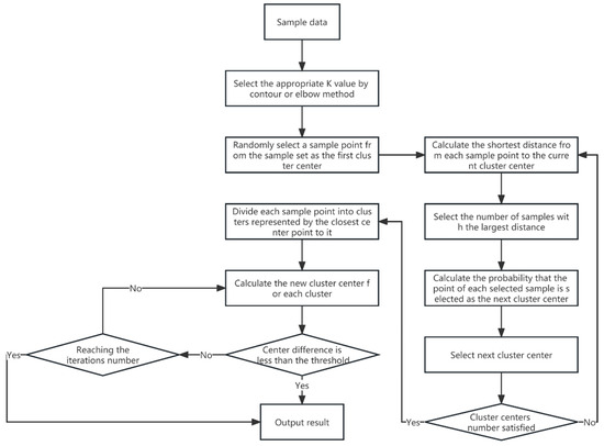
Figure 1.
The improved clustering algorithm.
Utilizing this enhanced approach, the electrical signals collected from operational electrical equipment are divided into multiple clusters. The distinct characteristics of these clusters provide insights into the varying behavioral patterns of different electrical equipment.
2.2. The Structure and Algorithm of a Bayesian Network
The Bayesian theory can be described as Equation (1) below.
where and are given events and are independent of each other. For a set of events , the probability of based on the conditional probability of is
The probability of can be derived using Equation (3).
The conditional probability of can be calculated with the prior probability and the independence probability.
After the cores of the data classification sample are determined, the distance from the sampled data to the core data can be used to represent the probability of being divided into related core points for the collected new data. In order to process that, the number of iterations for dimensionality reduction and the reduction target should be set after the input of a multidimensional data sample. Based on the equations given by Mwangi [41], the weight ω can be obtained using the equation
where G is the number of clusters and c is the distance between them. Then the weighted Euclidean distance can be described as
where and are the centers of the Gaussian distribution. Using weighted Euclidean distance to calculate the probability of similarity conditions between sample pairs in high-dimensional space can be described according to [42]
The variance parameter of the corresponding Gaussian function is determined in relation to the final number of nearest neighbors, determined so that P is higher when is closer to . In that case, the conditional probabilities can be calculated [43]. For the identification of electronic equipment, the categories are represented by the event of set , and each kind of identified symptom is represented by the event of . The probability that a kind of device may be used can be calculated when a certain condition is given.
A classic Bayesian network with two layers is shown in Figure 2. The network is built with nodes and directed arcs and is divided into two layers: the upper layer and the lower layer. Nodes in the upper layer are parent nodes, while nodes in the lower layer are child nodes, and they are connected by directed arcs.
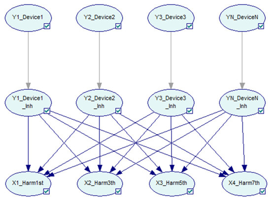
Figure 2.
A classic Bayesian network with directed arcs.
The network is constructed based on three independent assumptions:
- (a)
- All parent nodes are independent of each other.
- (b)
- If child nodes have no links to one another, all the child nodes of one certain parent node are independent of each other when the state of their parent node is given.
- (c)
- Any child node, when the state of its linked parent node is given, is independent of the parent nodes that have no direct links to it.
2.3. The Inhibitor Nodes and the Noisy-Max Gate
Based on the classic Bayesian network structure, a layer of inhibitor nodes is inserted in the middle of two layers, as shown in Figure 3.
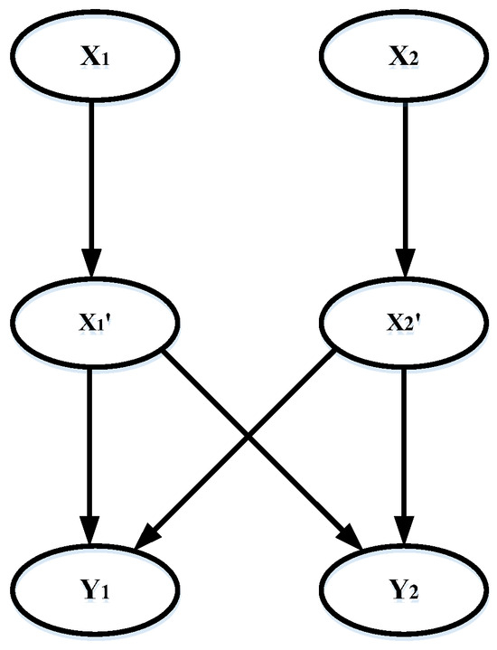
Figure 3.
The Bayesian network with inhibitor nodes and directed arcs.
Nodes in the inhibitor layer are represented by , with the same number as nodes in the first layer. Each inhibitor node corresponds to the one above it, and there is only one single directed link from the above node to it. The probabilistic relationships of cause and effect between a node in the first layer and a node in the inhibitor layer are established by the system noise of the network. The value of inhibitor nodes is set to the same value as those in the first layer [44].
The number of conditional probability tables in a classic Bayesian network, which should include all connections of states between child nodes and parent nodes, can grow exponentially with the number of nodes in the whole network. Given one child node with n parent nodes, the number of parameters is when each node is binary. For the Bayesian network with two parent nodes and two child nodes, there should be parameters when each node has only two states. The work of building a complete Bayesian network for load identification can be tremendous in this way.
The use of a Noisy-Max gate in the Bayesian network can reduce the parameter number effectively. For a network with one child node and parent nodes in the same situation as described above, only conditional probabilities should be set. There are three preconditions for the use of a Noisy-Max gate, which are:
- (a)
- At least one child node and its parent node contain the variables that include the current state.
- (b)
- Any parent node has a certain consequence for at least one child node.
- (c)
- Any parent node is independent of the other parent nodes.
Different states in nodes with a Noisy-Max gate are set and arranged with a certain rule. In the model, the states of each parent node are divided into three different levels: normal, lower, and higher, which can reflect the features of input signals. The inhibitor nodes are set to follow the first layer with the same states and order [45].
2.4. The Leak Probability
Since a large number of signal mechanisms are involved in the NILM, the diagnosis network cannot be built explicitly, containing every possible factor. The symptoms of fault that may not be established as nodes in the Bayesian network should be considered. Leak probability can solve that problem in the diagnosis model, improving accuracy. In the Bayesian network, a leak node is added as a parent node , as shown in the upper layer (Figure 4).
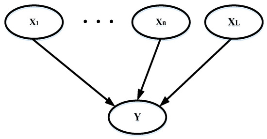
Figure 4.
A Bayesian network with leak probability node.
The causes that are not included by any other parent nodes are set by the node , which can trigger the child node. For the Bayesian network shown in Figure 4, there is
given that
According to Zagorecki [44], it can be concluded that
where T represents the true state while F represents the false state, and the node of truth is presented by . So
The can be obtained using Equation (12).
The conditional probability distributions with leak probability can be calculated using Equation (13).
The type of device can be determined when the identification probability is greater than a certain threshold, . The threshold is a constant value and can be optimized during the process. It is suggested that it be set at 80% at the initial stage [46].
By using the Bayesian network model, the obtained electrical signals are analyzed. When the probability value of the output result of a certain electrical device exceeds the set threshold, it can be determined that the signal contains the operating characteristics of the device, and the device is in operation at this time.
3. Experiments
To validate the accuracy of the load recognition algorithm proposed in this study, simulation experiments were conducted to collect electric signal data in a controlled laboratory setting. The experiments took place in the Intelligent Kitchen Electrical Behavior Analysis Laboratory, a facility funded and established by the Innovation Research Institute of Zhejiang University of Technology, located in Shengzhou City, Zhejiang Province, China. This laboratory is dedicated to simulating the operational scenarios of electrical equipment as well as conducting data acquisition and analysis of electrical behavior. It serves as a comprehensive analysis hub, integrating simulation of electrical equipment usage scenarios, collection of electrical behavior data, and analysis of electrical behavior characteristics. A depiction of the laboratory layout is presented in the accompanying figure.
The laboratory is outfitted with a variety of common household appliances for analytical purposes, alongside non-intrusive electrical behavior analysis equipment. It is sectioned into three functional areas: the experimental area, the data collection area, and the analysis area. Electrical signals during the operation of equipment are captured based on simulated daily operations.
The power supply in the laboratory is facilitated using an ITECH High-Power Programmable AC Source IT7805 (product of ITECH Electronic Co., Ltd., Suzhou, China). A FLUKE 1738 Power Quality Logger (product of Fluke Corporation, Washington, United States), which monitors and records electrical signal data, is employed during the simulated operational processes. Prior to signal capture, the power supply is set to the standard, aligning with the power consumption norms in China. Current signals are collected using sensing clamps, while voltage data are acquired through parallel connections. During the experimental phase, the recorder is equipped with a 16 A current clamp capable of sampling rates up to 10 kHz. To prevent data overload and potential data collapse, the sampling frequency is set at 0.5 kHz, equating to data collection every 0.002 s. In the data processing phase, the computer utilized is equipped with a 12th Gen Intel(R) Core(TM) i7 CPU (product of Lenovo, Beijing, China), with a base clock speed of 2.10 GHz. The high sampling rate ensures prompt computational results following the initiation of the devices. The captured electrical signals are then transmitted to a computer for analysis using the methods described earlier.
In this experiment, the microwave oven, one of the most commonly used household electrical appliances, was chosen as the focus for research and analysis. Two different brands of microwave ovens, Galanz (Galanz Corporation, Shunde, China) and Midea (Midea Corporation, Foshan, China), which are top sellers in China, were selected for testing and validation. Details of the two microwave oven models are provided in Table 1 below.

Table 1.
Detail of two tested microwave ovens.
The experimental setup, as shown in Figure 5, illustrates the interconnection of various relevant pieces of equipment. Initially, the AC power source was connected to a power strip, which served as the primary source of electricity for the experiment. The device under test, namely the microwave oven, was also plugged into this power strip. This strip acts as a busbar for all devices, from which they derive electrical energy. A current clamp was then attached to the live wire of the power strip, and a wire leading to a plug was inserted into the strip as well. Both were connected to the recorder, as depicted in Figure 6. This setup enables the collection of corresponding current and voltage signals. The AC power source was set to output 220 V and 50 Hz, fulfilling the microwave oven’s rated input requirements.
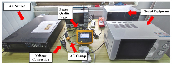
Figure 5.
The experiment equipment.
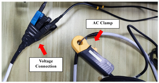
Figure 6.
The data acquisition of microwave oven.
To ensure comprehensive data collection, the recording device was programmed to start logging data before the activation of the power supply, capturing the entire operational cycle of the microwave oven. During testing, cold food items were introduced into the microwave to replicate typical food-heating scenarios found in household kitchens. These tests were conducted in a specially designed cubicle, replicating the dimensions of a standard household kitchen to maximize ecological validity. Throughout the experimental process, the microwave oven was operated at three distinct settings: low, medium, and high. Electrical signals corresponding to each setting were meticulously recorded.
Following the acquisition of operational electrical signals from a Galanz microwave oven, the sampled signals were analyzed to determine power values, fundamental current signals, and odd harmonics, specifically the 1st, 3rd, 5th, and 7th harmonics. Power trend graphs facilitated the segmentation and determination of operational events within the microwave oven’s working cycle. For three different operating modes, microwave oven operation events were segmented based on the power figures below, allowing for the determination of the start and end times of each event. As illustrated in Figure 7 below, the segments between points A and B and C and D in each power graph represent sub-events within the microwave oven’s operation.
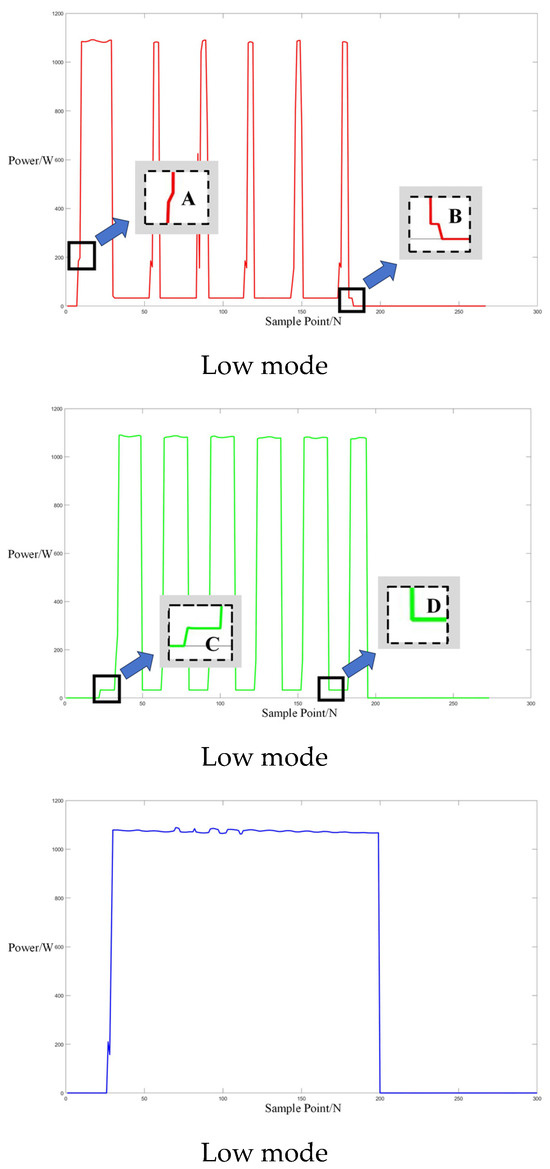
Figure 7.
Three operation power modes of Galanz microwave oven.
After the event identification, an analysis of the electrical current signals was conducted during the operational process, focusing on identifying the central clusters for the 1st, 3rd, 5th, and 7th harmonics. For the Galanz microwave oven operating at low, medium, and high settings, the central cluster positions for these harmonics are detailed in the figures in Appendix A, Figure A1, Figure A2 and Figure A3, shown below. The central cluster positions for these harmonics are detailed in Table 2, shown below.
Table 2.
Central cluster positions of harmonics of Galanz microwave oven.
A Bayesian network model with inhibitory nodes was then constructed based on the current signal characteristics, as shown in Figure 8. The upper layer of the model identifies the appliance type, in this case, a microwave oven, while the lower layer comprises signal characteristic nodes, including total power and current harmonics for the 1st, 3rd, 5th, and 7th harmonics. Inhibitory and leak nodes in the model are utilized for calculation purposes and are not explicitly shown in the diagram.
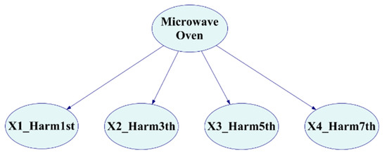
Figure 8.
Bayesian structure layers.
Upon receiving electrical signal input, the established network model calculates node probability values, enabling the identification of the microwave oven’s operational status.
To further verify the accuracy of the proposed method, a Midea microwave oven was used in simulated experiments. These experiments included scenarios of the microwave oven operating independently, in conjunction with other household appliances, and with other appliances operating while the microwave oven remained inactive.
3.1. Independent Operation of the Microwave Oven
Upon acquiring operational electrical signals from the Midea microwave oven, the collected signals were segmented into electrical behavior events. As indicated by the arrows in Figure 9 below, segments between points A and B, C and D, and E and F represent sub-events in the microwave’s operation.
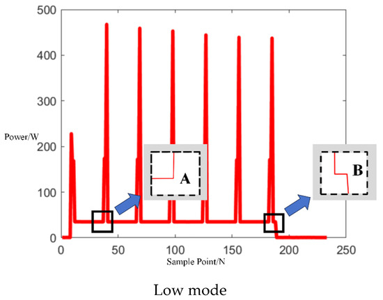
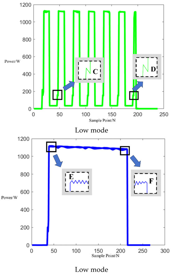
Figure 9.
Three operation power modes of Midea microwave oven of independent operation.
After event identification, an analysis of the current signals was conducted to determine central clusters for the 1st, 3rd, 5th, and 7th harmonics, as detailed in the figure in Appendix A, Figure A4, Figure A5 and Figure A6; each cluster position is summarized in Table 3.
Table 3.
Central cluster positions of harmonics of Midea microwave oven.
The Euclidean distances from the data center of each current signal to the predetermined centers are listed in Table 4.
Table 4.
The Euclidean distances of each current signal to the predetermined center of Midea microwave oven.
Utilizing the previously mentioned formula, the probability values for each power setting of the microwave oven were calculated as shown in Table 5.
Table 5.
Results of calculated probabilities.
The resulting usage probability values exceeded the predefined threshold ε, indicating successful identification of the microwave oven’s operational status in all three experiments.
3.2. Mixed Appliance Operation, Including Microwave Oven
The process of signal segmentation and event determination was similar to the previous scenario. Sub-events can be represented between points A and B, C and D, E and F, and G and H based on the power trends of mixed appliance operation, including the microwave oven, as shown in Figure 10. The timetable of the appliance state is shown in Appendix A, Table A1.
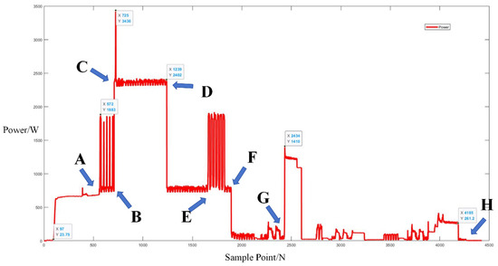
Figure 10.
Power trends of mixed appliance operation, including microwave oven.
After event identification, the analysis of the current signals was conducted to determine central clusters for the 1st, 3rd, 5th, and 7th harmonics, as detailed in Figure 11. The central cluster positions for the current fundamental and odd harmonics during the operation are detailed in Table 6, and the Euclidean distances of each current signal are summarized in Table 7.
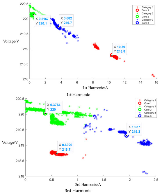
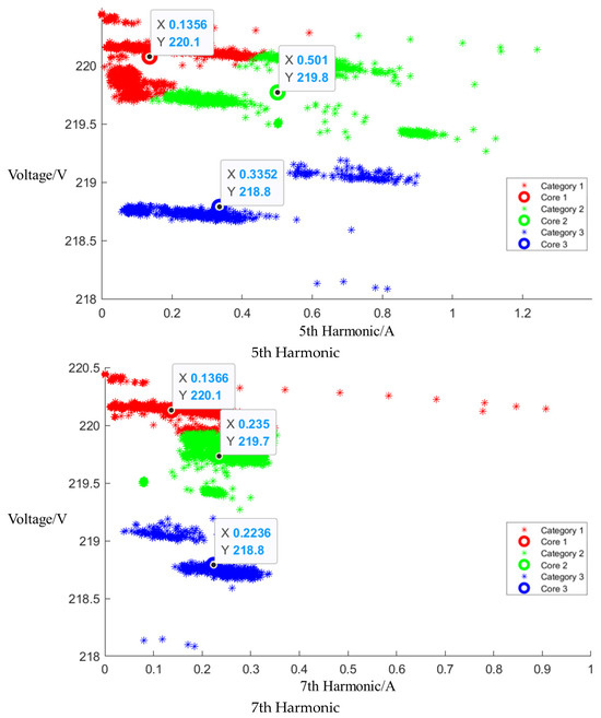
Figure 11.
Cluster of mixed appliance operation, including microwave oven.
Table 6.
Central cluster positions of harmonics of mixed appliance operation, including microwave oven.
Table 7.
The Euclidean distances of each current signal to the predetermined center of mixed appliance operation, including microwave oven.
The Bayesian network model, as previously described, was employed to calculate the probability values for each power setting of the microwave oven. The calculated probabilities, which is 98.4% for low mode, 54.2% for medium mode, and 28.3% for high mode, suggested the microwave oven was in use, most likely operating at a low power setting.
3.3. Mixed Appliance Operation, Excluding Microwave Oven
This scenario followed a similar process of signal segmentation and event determination. Sub-events can be represented between points A and B, C and D, and E and F based on the power trends of mixed appliance operation, excluding the microwave oven, as shown in Figure 12. Figure 13 shows the results of the analysis conducted to determine central clusters for the 1st, 3rd, 5th, and 7th harmonics, and Table 8 lists the central cluster positions for the current fundamental and odd harmonics, while Table 9 lists the Euclidean distances of each current signal.
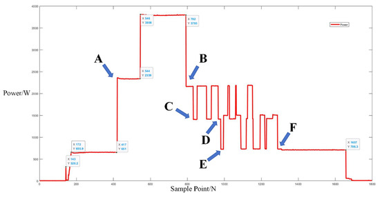
Figure 12.
Power trends of mixed appliance operation, excluding microwave oven.
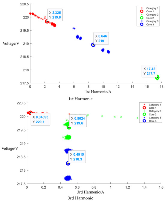
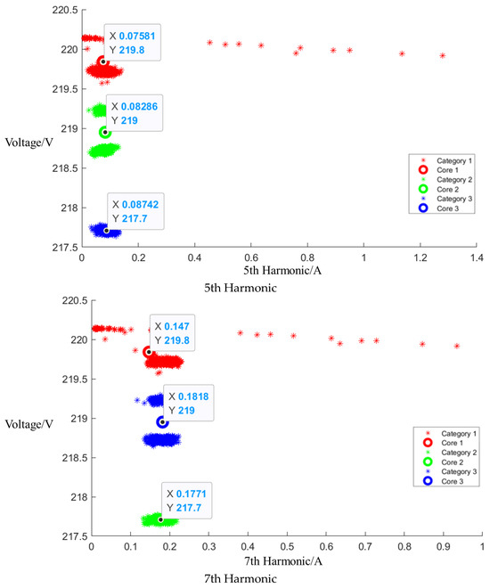
Figure 13.
Cluster of mixed appliance operation, excluding microwave oven.
Table 8.
Central cluster positions of harmonics of mixed appliance operation, excluding microwave oven.
Table 9.
The Euclidean distances of each current signal to the predetermined center of mixed appliance operation, excluding microwave oven.
The central cluster positions for the current fundamental and odd harmonics are detailed in the table below. Using the established Bayesian network model, the probability values of 32.4% for low mode, 30.2% for medium mode, and 37.7% for high mode for each power setting of the microwave oven were calculated. These values indicated that the microwave oven was not in operation during this scenario.
4. Result Discussion
In this study, relevant electrical signals were obtained through simulated experiments with microwave ovens under three distinct operational scenarios. These signals were then processed through a Bayesian network model developed to calculate the probability values for each experimental outcome. The results indicate that for the same electrical appliance, the model successfully identified the operational states at low, medium, and high settings, with probability values exceeding the decision threshold (low mode 89.1%, medium mode 94.4%, high mode 92.0%). When the microwave oven operated concurrently with other electrical devices, the model accurately determined its operational state probabilities (low mode 98.4%, medium mode 54.2%, high mode 28.3%). Furthermore, in scenarios excluding microwave usage with other appliances in operation, the inferred probabilities decreased significantly, suggesting non-usage of the microwave (low mode 32.4%, medium mode 30.2%, high mode 37.7%). These experimental outcomes validate the theoretical effectiveness of the proposed method.
Compared to existing state recognition methodologies using clustering and Bayesian networks [47], the proposed approach demonstrates certain improvements. The criteria for state inference have been expanded and refined. Instead of relying solely on current or power values for determination, the proposed method employs a decision-making process based on the fundamental current and multiple harmonics, coupled with an improved clustering method to identify cluster centroids. This approach more accurately captures the core characteristics of electrical appliance usage, enabling more precise determinations. For validation, we conducted inference processes under the same operational conditions, using only current or power values. While the microwave oven’s operational current and power were set as activation conditions for the network nodes, resulting in a high identification probability of 98.9% in solitary operation, the probability fluctuated around 50% in mixed operation modes. This indicates that relying solely on current or power values could lead to misjudgments and an inability to determine the current mode accurately. In contrast to other methodologies that only provide conclusive determinations, our approach precisely calculates probability values based on node activation states, offering a clearer understanding and a more accurate response for the electrical behavior management of devices.
For future research, there is potential to further expand the categorization of appliance operational states and the establishment of additional network nodes.
5. Conclusions
This study focuses on acquiring electrical current signals during the operation of devices through the non-intrusive load monitoring (NILM) approach. Based on extracting the fundamental current and harmonics (3rd, 5th, and 7th), we employed a refined K-means clustering method to locate the centers of signal clusters. The Euclidean distances from these cluster centers were then used to construct a Bayesian network model. The model calculates the probability of a device being in operation based on the activation status of each harmonic node. Verificatory experiments were conducted in the laboratory with a microwave oven as the subject of study. These experimental outcomes, as shown in Section 4, validate the theoretical efficacy of the proposed approach.
Author Contributions
Conceptualization, Y.X.; methodology, L.X.; software, C.W.; validation, M.W.; writing—original draft preparation, J.L.; writing—review and editing, J.L. and Y.X. All authors have read and agreed to the published version of the manuscript.
Funding
This research was funded by Scientific Research Fund of Zhejiang Provincial Education Department, Y202352521, the National Natural Science Foundation of China, 52105217, and the Natural Science Foundation of Zhejiang Province, LQ22E050020.
Institutional Review Board Statement
Not applicable.
Informed Consent Statement
Not applicable.
Data Availability Statement
The data presented in this study are available on request from the corresponding author.
Conflicts of Interest
The authors declare no conflicts of interest.
Correction Statement
This article has been republished with a minor correction to the Funding statement. This change does not affect the scientific content of the article.
Appendix A


Figure A1.
Cluster of Galanz microwave oven operating at low setting.
Figure A1.
Cluster of Galanz microwave oven operating at low setting.


Figure A2.
Cluster of Galanz microwave oven operating at medium setting.
Figure A2.
Cluster of Galanz microwave oven operating at medium setting.


Figure A3.
Cluster of Galanz microwave oven operating at high setting.
Figure A3.
Cluster of Galanz microwave oven operating at high setting.


Figure A4.
Cluster of Media microwave oven operating at low setting.
Figure A4.
Cluster of Media microwave oven operating at low setting.


Figure A5.
Cluster of Media microwave oven operating at medium setting.
Figure A5.
Cluster of Media microwave oven operating at medium setting.


Figure A6.
Cluster of Media microwave oven operating at high setting.
Figure A6.
Cluster of Media microwave oven operating at high setting.


Table A1.
Timetable for appliance mix with microwave oven.
Table A1.
Timetable for appliance mix with microwave oven.
| 9:35 | 9:40 | 9:43 | 9:46 | 10:01 | 10:04 | 10:05 | 10:14 | 10:20 | 10:45 |
|---|---|---|---|---|---|---|---|---|---|
| AC on | Wash machine on | Microwave oven on | Microwave oven off | Microwave oven on | Microwave oven off | AC adjust | Microwave oven on | AC off | Wash machine off, microwave oven off |
Table A2.
Timetable for appliance mix without microwave oven.
Table A2.
Timetable for appliance mix without microwave oven.
| 15:20 | 15:25 | 15:27 | 15:31 | 15:40 | 15:45 |
|---|---|---|---|---|---|
| AC on | Kettle on | Oven on | Kettle off | Oven off | AC off |
References
- Administration UEEI. Annual Energy Review. 2022. Available online: www.eia.gov/totalenergy/data/annual/ (accessed on 14 August 2023).
- Hart, G.W. Nonintrusive appliance load monitoring. Proc. IEEE 1992, 80, 1870–1891. [Google Scholar] [CrossRef]
- Chang, H.H.; Lin, C.L.; Yang, H.T. Load recognition for different loads with the same real power and reactive power in a non-intrusive load-monitoring system. In Proceedings of the 2008 12th International Conference on Computer Supported Cooperative Work in Design, Xi’an, China, 16–18 April 2008. [Google Scholar]
- Aladesanmi, E.J.; Folly, K.A. Overview of non-intrusive load monitoring and identification techniques. IFAC-Pap. 2015, 48, 415–420. [Google Scholar] [CrossRef]
- Sultanem, F. Using appliance signatures for monitoring residential loads at meter panel level. IEEE Trans. Power Deliv. 1991, 6, 1380–1385. [Google Scholar] [CrossRef]
- Lee, K.; Leeb, S.; Norford, L.; Armstrong, P.; Holloway, J.; Shaw, S. Estimation of variable-speed-drive power consumption from harmonic content. IEEE Trans. Energy Convers. 2005, 20, 566–574. [Google Scholar] [CrossRef]
- Laughman, C.; Lee, K.; Cox, R.; Shaw, S.; Leeb, S.; Norford, L.; Armstrong, P. Power signature analysis. IEEE Power Energy Mag. 2003, 1, 56–63. [Google Scholar] [CrossRef]
- Khan, U.; Leeb, S.; Lee, M. A multiprocessor for transient event detection. IEEE Trans. Power Deliv. 1997, 12, 51–60. [Google Scholar] [CrossRef]
- Norford, L.K.; Leeb, S.B. Non-intrusive electrical load monitoring in commercial buildings based on steady-state and transient load-detection algorithms. Energy Build. 1996, 24, 51–64. [Google Scholar] [CrossRef]
- Leeb, S.; Shaw, S.; Kirtley, J. Transient event detection in spectral envelope estimates for nonintrusive load monitoring. IEEE Trans. Power Deliv. 1995, 10, 1200–1210. [Google Scholar] [CrossRef]
- Hassan, T.; Javed, F.; Arshad, N. An empirical investigation of VI trajectory based load signatures for non-intrusive load monitoring. IEEE Trans. Smart Grid 2013, 5, 870–878. [Google Scholar] [CrossRef]
- He, D.; Du, L.; Yang, Y.; Harley, R.; Habetler, T. Front-end electronic circuit topology analysis for model-driven classification and monitoring of appliance loads in smart buildings. IEEE Trans. Smart Grid 2012, 3, 2286–2293. [Google Scholar] [CrossRef]
- Bouhouras, A.S.; Gkaidatzis, P.A.; Panagiotou, E.; Poulakis, N.; Christoforidis, G.C. A NILM algorithm with enhanced disaggregation scheme under harmonic current vectors. Energy Build. 2019, 183, 392–407. [Google Scholar] [CrossRef]
- Wanik, M. Harmonic measurement and analysis during electric vehicle charging. Engineering 2013, 5, 215–220. [Google Scholar] [CrossRef]
- Djordjevic, S.; Simic, M. Nonintrusive identification of residential appliances using harmonic analysis. Turk. J. Electr. Eng. Comput. Sci. 2018, 26, 780–791. [Google Scholar] [CrossRef]
- Srinivasan, D.; Ng, W.; Liew, A. Neural-network-based signature recognition for harmonic source identification. IEEE Trans. Power Deliv. 2005, 21, 398–405. [Google Scholar] [CrossRef]
- Wang, C.; Wu, Z.; Peng, W.; Liu, W.; Xiong, L.; Wu, T.; Yu, L.; Zhang, H. Adaptive modeling for non-intrusive load monitoring. Int. J. Electr. Power Energy Syst. 2022, 140, 107981. [Google Scholar] [CrossRef]
- Grover, H.; Panwar, L.; Verma, A.; Panigrahi, B.; Bhatti, T. A multi-head Convolutional Neural Network based non-intrusive load monitoring algorithm under dynamic grid voltage conditions. Sustain. Energy Grids Netw. 2022, 32, 100938. [Google Scholar] [CrossRef]
- Green, C.; Garimella, S. Analysis of supervised graph signal processing-based load disaggregation for residential demand-side management. Electr. Power Syst. Res. 2022, 208, 107878. [Google Scholar] [CrossRef]
- Aslan, M.; Zurel, E.N. An efficient hybrid model for appliances classification based on time series features. Energy Build. 2022, 266, 112087. [Google Scholar] [CrossRef]
- Nie, Z.; Yang, Y.; Xu, Q. An ensemble-policy non-intrusive load monitoring technique based entirely on deep feature-guided attention mechanism. Energy Build. 2022, 273, 112356. [Google Scholar] [CrossRef]
- Qu, L.; Kong, Y.; Li, M.; Dong, W.; Zhang, F.; Zou, H. A residual convolutional neural network with multi-block for appliance recognition in non-intrusive load identification. Energy Build. 2023, 281, 112749. [Google Scholar] [CrossRef]
- Yan, L.; Sheikholeslami, M.; Gong, W.; Tian, W.; Li, Z. Challenges for real-world applications of nonintrusive load monitoring and opportunities for machine learning approaches. Electr. J. 2022, 35, 107136. [Google Scholar] [CrossRef]
- Ghosh, S.; Chatterjee, A.; Chatterjee, D. Extraction of statistical features for type-2 fuzzy NILM with IoT enabled control in a smart home. Expert Syst. Appl. 2023, 212, 118750. [Google Scholar] [CrossRef]
- Keramati, M.M.; Azizi, E.; Momeni, H.; Bolouki, S. Incorporating coincidental water data into non-intrusive load monitoring. Sustain. Energy Grids Netw. 2022, 32, 100805. [Google Scholar] [CrossRef]
- Luan, W.; Yang, F.; Zhao, B.; Liu, B. Industrial load disaggregation based on hidden Markov models. Electr. Power Syst. Res. 2022, 210, 108086. [Google Scholar] [CrossRef]
- Li, C.; Zheng, K.; Guo, H.; Chen, Q. A mixed-integer programming approach for industrial non-intrusive load monitoring. Appl. Energy 2023, 330, 120295. [Google Scholar] [CrossRef]
- Cui, J.; Jin, Y.; Yu, R.; Okoye, M.O.; Li, Y.; Yang, J.; Wang, S. A robust approach for the decomposition of high-energy-consuming industrial loads with deep learning. J. Clean. Prod. 2022, 349, 131208. [Google Scholar] [CrossRef]
- Xu, Y.; Wang, J.; Shen, X.; Sun, Z.; Wang, X.; Han, X. Thermodynamic analyses and performance improvement on a novel cascade-coupling-heating heat pump system for high efficiency hot water production. Energy Convers. Manag. 2023, 293, 117448. [Google Scholar] [CrossRef]
- Xu, Y.; Xie, Y.; Wang, X.; Shen, X.; Song, M.; Hang, W. Study on a novel defrost control method based on the surface texture of evaporator image with gray-level cooccurrence matrix, new characterization parameter combination and machine learning. Energy Build. 2023, 292, 113173. [Google Scholar] [CrossRef]
- Serafini, L.; Tanoni, G.; Principi, E.; Spinsante, S.; Squartini, S. A multiple instance regression approach to electrical load disaggregation. In Proceedings of the 2022 30th European Signal Processing Conference (EUSIPCO), Belgrade, Serbia, 29 August–2 September 2022; pp. 1666–1670. [Google Scholar]
- Mari, S.; Bucci, G.; Ciancetta, F.; Fiorucci, E.; Fioravanti, A. A Review of Non-Intrusive Load Monitoring Applications in Industrial and Residential Contexts. Energies 2022, 15, 9011. [Google Scholar] [CrossRef]
- Mehmood, A.; Sajjad, I.A.; Ullah, M.N.; Liaqat, R.; Abbas, M.Z.; Wasaya, A. Evaluation of Feature Selection Methods for Non-Intrusive Load Monitoring. In Proceedings of the 2021 International Conference on Technology and Policy in Energy and Electric Power (ICT-PEP), Jakarta, Indonesia, 29–30 September 2021; pp. 324–329. [Google Scholar]
- Souza, W.A.; Alonso, A.M.; Bosco, T.B.; Garcia, F.D.; Gonçalves, F.A.; Marafão, F.P. Selection of features from power theories to compose NILM datasets. Adv. Eng. Inform. 2022, 52, 101556. [Google Scholar] [CrossRef]
- Souza, W.A.; Marafão, F.P.; Liberado, E.V.; Simões, M.G.; Da Silva, L.C. A nilm dataset for cognitive meters based on conservative power theory and pattern recognition techniques. J. Control Autom. Electr. Syst. 2018, 29, 742–755. [Google Scholar] [CrossRef]
- Athanasiadis, C.; Doukas, D.; Papadopoulos, T.; Chrysopoulos, A. A scalable real-time non-intrusive load monitoring system for the estimation of household appliance power consumption. Energies 2021, 14, 767. [Google Scholar] [CrossRef]
- Yu, Q.; Liu, Y.; Jiang, Z.; Xu, C.; Yang, R.; Zhang, R. Research of load behavior based on NILM in domestic microgrid. In Proceedings of the 2020 15th IEEE International Conference on Signal Processing (ICSP), Beijing, China, 6–9 December 2020; Volume 1, pp. 337–340. [Google Scholar]
- Papageorgiou, P.G.; Christoforidis, G.C.; Bouhouras, A.S. Odd Harmonic Distortion Contribution on a Support Vector Machine NILM Approach. In Proceedings of the 2022 2nd International Conference on Energy Transition in the Mediterranean Area (SyNERGY MED), Thessaloniki, Greece, 17–19 October 2022; pp. 1–6. [Google Scholar]
- Etezadifar, M.; Karimi, H.; Mahseredjian, J. Non-intrusive load monitoring: Comparative analysis of transient state clustering methods. Electr. Power Syst. Res. 2023, 223, 109644. [Google Scholar] [CrossRef]
- Tambunan, H.B.; Barus, D.H.; Hartono, J.; Alam, A.S.; Nugraha, D.A.; Usman, H.H.H. Electrical peak load clustering analysis using K-means algorithm and silhouette coefficient. In Proceedings of the 2020 International Conference on Technology and Policy in Energy and Electric Power (ICT-PEP), Bandung, Indonesia, 23–24 September 2020; pp. 258–262. [Google Scholar]
- Mwangi, B.; Soares, J.C.; Hasan, K.M. Visualization and unsupervised predictive clustering of high-dimensional multimodal neuroimaging data. J. Neurosci. Methods 2014, 236, 19–25. [Google Scholar] [CrossRef] [PubMed]
- Van der Maaten, L.; Hinton, G. Visualizing data using t-SNE. J. Mach. Learn. Res. 2008, 9, 2579–2605. [Google Scholar]
- Srinivasarengan, K.; Goutam, Y.G.; Chandra, M.G.; Kadhe, S. A framework for non intrusive load monitoring using bayesian inference. In Proceedings of the 2013 Seventh International Conference on Innovative Mobile and Internet Services in Ubiquitous Computing, Taichung, Taiwan, 3–5 July 2013; pp. 427–432. [Google Scholar]
- Zagorecki, A.; Druzdzel, M.J. Knowledge engineering for Bayesian networks: How common are noisy-MAX distributions in practice? IEEE Trans. Syst. Man Cybern. Syst. 2012, 43, 186–195. [Google Scholar] [CrossRef]
- Díez, F.J.; Galán, S.F. Efficient computation for the noisy MAX. Int. J. Intell. Syst. 2003, 18, 165–177. [Google Scholar] [CrossRef]
- Zhao, Y.; Xiao, F.; Wang, S. An intelligent chiller fault detection and diagnosis methodology using Bayesian belief network. Energy Build. 2013, 57, 278–288. [Google Scholar] [CrossRef]
- Henao, N.; Agbossou, K.; Kelouwani, S.; Hosseini, S.S.; Fournier, M. Power estimation of multiple two-state loads using a probabilistic non-intrusive approach. Energies 2018, 11, 88. [Google Scholar] [CrossRef]


Disclaimer/Publisher’s Note: The statements, opinions and data contained in all publications are solely those of the individual author(s) and contributor(s) and not of MDPI and/or the editor(s). MDPI and/or the editor(s) disclaim responsibility for any injury to people or property resulting from any ideas, methods, instructions or products referred to in the content. |
© 2024 by the authors. Licensee MDPI, Basel, Switzerland. This article is an open access article distributed under the terms and conditions of the Creative Commons Attribution (CC BY) license (https://creativecommons.org/licenses/by/4.0/).