Efficient Diagnosis of Autism Spectrum Disorder Using Optimized Machine Learning Models Based on Structural MRI

Abstract

Autism spectrum disorder (ASD) affects approximately 1.4% of the population and imposes significant social and economic burdens. Because its etiology is unknown, effective diagnosis is challenging. Advancements in structural magnetic resonance imaging (sMRI) allow for the objective assessment of ASD by examining structural brain changes. Recently, machine learning (ML)-based diagnostic systems have emerged to expedite and enhance the diagnostic process. However, the expected success in ASD was not yet achieved. This study evaluates and compares the performance of seven optimized ML models to identify sMRI-based biomarkers for early and accurate detection of ASD in children aged 5 to 10 years. The effect of using hyperparameter tuning and feature selection techniques are investigated using two public datasets from Autism Brain Imaging Data Exchange Initiative. Furthermore, these models are tested on a local Saudi dataset to verify their generalizability. The integration of the grey wolf optimizer with a support vector machine achieved the best performance with an average accuracy of 71% (with further improvement to 71% after adding personal features) using 10-fold Cross-validation. The optimized models identified relevant biomarkers for diagnosis, lending credence to their truly generalizable nature and advancing scientific understanding of neurological changes in ASD.

1. Introduction

Autism spectrum disorder (ASD) affects 1.5% of children worldwide, being 4.5 times more prevalent in males than in females [1]. In 2023, the estimated prevalence of ASD in the United States is 80.9 per 10,000 people, while in Saudi Arabia, it is 100.7 per 10,000 people, reflecting similar patterns observed in many countries [2,3]. ASD is a developmental disorder marked by early social communication and interaction impairments, along with restricted and repetitive activities and interests [4]. The term “spectrum” refers to the variation in the severity and form of symptoms, which were classified as separate disorders before the publication of the fifth edition of the Diagnostic and Statistical Manual of Mental Disorders (DSM-5) [5]. Symptoms appear in early childhood and continue throughout life, resulting in challenges such as learning difficulties, increased psychological pressures on families, and social isolation. The cause of ASD remains unknown, making effective treatment challenging. However, early diagnosis enables healthcare providers and families to implement early interventions that enhance the quality of life for individuals with autism. Presently, diagnostic approaches rely heavily on behavioral characterization, which is time-consuming, expensive, susceptible to bias, and often does not meet DSM-5 evaluation criteria. Moreover, due to comorbidity, these approaches may be inconclusive [5].

Structural magnetic resonance imaging (sMRI) is a non-invasive technique to study brain morphology and diagnose disorders, particularly in children. It provides high contrast sensitivity and resolution without radiation [6]. sMRI is used to obtain different brain tissue sequences, such as T1 and T2. Longitudinal studies also utilize sMRI to monitor brain growth over time [7]. Moreover, the big brain theory [8] has a structural basis, positing that autistic people have larger brains than their peers with typical development (TD). However, older statistical methods for studying structural changes in brain regions are univariate and based on group differences, which cannot be directly related to clinical diagnosis based on biomarker identification for an individual [9].

Machine learning (ML) has recently contributed to building efficient computer-aided diagnostic (CAD) systems, analyzing complex medical imaging and Big Data in less time and eliminating human errors. It also facilitates studies at the individual level and acts as a vector with multiple variables [5]. ML models using data can automatically predict and diagnose ASD earlier, improving the lives of patients and their families and reducing financial costs. Personal and behavioral features, along with sMRI data, are valuable resources for ML algorithms in uncovering hidden patterns for disorder prediction. However, challenges arise from hyperparameters and high-dimensional data, making algorithm operation difficult. Optimization approaches like random search methods, feature selection (FS), and hyperparameter tuning can enhance algorithm development, accelerate classification, reduce costs, address high dimensionality, and improve prediction model accuracy [10].

There are three common types of FS algorithm: filter, wrapper, and embedded, which aim to select the most important and effective features for prediction problems. New optimization techniques, such as bio-inspired algorithms, can enhance FS methods by globally searching for the optimal feature subset and improving prediction accuracy [11]. ML has shown significant benefits in accurate ASD diagnosis, saving time and effort for human experts and facilitating effective intervention. Despite recent attention, further improvement is needed in this area, and more research is required for classifying ASD using enhanced algorithms. To our knowledge, this study is the first to employ the nature-inspired grey wolf optimizer (GWO) algorithm and the Boruta algorithm for sMRI-based ASD classification.

This work aims to enhance the early classification accuracy of ASD using high-dimensional sMRI data for children aged 5 to 10 years, as well as to identify important biomarkers associated with ASD. To achieve this, a comparative empirical study is conducted using different optimization algorithms combined with seven ML algorithms using two public datasets from the Autism Brain Imaging Data Exchange Initiative (ABIDE) and local data from King Abdulaziz University (KAU) Hospital. To our knowledge, the KAU dataset is the first Saudi dataset used in ML applications for ASD classification. Recursive feature elimination with cross-validation (RFECV), Boruta and GWO-based algorithms for FS, and random search algorithm and GWO algorithm for hyperparameter tuning were all investigated. The impact of age and gender on classification performance is also examined. This study addresses the following research questions:

• Can the proposed FS methods improve the accuracy of ML models in ASD classification?
• Which of the proposed optimized models performs the best in predicting ASD in terms of accuracy on the two public datasets?
• Does combining personal features data with sMRI yield better results in ASD classification compared to using only sMRI data?

The reminder of this paper is organized as follows. Section 2 reviews the related work. Section 3 describes the materials and methods employed in this study. In Section 4, we present and discuss the results and limitations of the research and suggest future work. Finally, Section 5 summarizes and concludes the paper.

2. Related Work

ML encompasses computational techniques using data for learning, performance improvement, and prediction. Although ASD classification methods can vary, Figure 1 illustrates the common steps involved in developing ML applications, including: (a) data collection and preprocessing; (b) feature extraction and selection; (c) model training; and (d) model testing and performance evaluation.

Earlier studies on ASD categorization primarily focused on ML or deep learning (DL) techniques. Bahathiq et al. analyzed 45 articles proposing ML-based methods for ASD diagnosis using sMRI [5]. These studies differed in ML algorithms, hyperparameters values, sample size, and input features. There are very few publicly available datasets, with the ABIDE datasets being the most well-known. Typically, individual ML algorithms such as support vector machine (SVM) [12,13], Naïve Bayes (NB) [14], or k-nearest neighbor [15] were investigated in these studies. Ref. [16] used extreme gradient boosting (XGB) with ABIDE I male samples within a narrow age range, which limits generalizability to other age groups. Challenges increased when using the entire large dataset due to sample variability [17]. In the quest for biomarkers, various local and global parameters of the brain, such as white matter (WM) volumes and cortical thickness (CT), have been utilized [18,19].

In [20], seven morphological features from 67 subjects were used, and the best accuracy was obtained using average CT for each of 68 regions of interest (ROIs). Bilgen et al. [21] evaluated twenty ML approaches based on morphological brain networks (MBNs) by considering preprocessing steps, dimensionality reduction techniques, and learning methods. The top two teams achieved accuracies of 70% and 63.8% using the gradient boosting classifier (GBC). Several ML models have been used to distinguish autistic from TD participants using either sMRI alone [12] or sMRI combined with other data [22]. Katuwal et al. [23] demonstrated the potential for early detection of ASD before the age of 10 using a random forest (RF) model on MRI features of male brains. Participants from the ABIDE I and II datasets were divided into four groups based on gender and health problems (TD or ASD) in [24] to investigate gender differences in ASD diagnosis. Following that, an ML model was trained using various combinations of functional and structural attributes.

A DL model identified ASD with an accuracy of 65.6% in [25] using resting-state fMRI (rs-fMRI), white matter (WM), and gray matter (GM) features from the two ABIDE datasets. Unlike the early-life global volume increases in ASD, the volume of GM/WM varies in adult brain regions, increasing and decreasing. As a result, previous studies on ASD biomarkers yielded contradictory results. In [26], an end-to-end framework was offered which uses 14 models that are compounds of different network architectures, among them a static CNN model, sequential learning models (e.g., RNN), Spatial Transformer Networks, and feature visualization methods (such as CAM). For a private dataset, the authors discovered that the 2D3D CNN and RAM worked best, whereas for the ABIDE dataset, a basic 3D CNN performed best. The highest ACC of this study was 61.7%.

Previous studies have shown promise in using ML algorithms for investigating ASD. However, these studies had limitations. First, many investigations trained a single model on small, high-dimensional MRI datasets, leading to overfitting and unstable models. Additionally, the generalizability of these models was questionable as they were not evaluated on external datasets [27]. Second, important biomarkers and neurophysiological significance of findings were not thoroughly analyzed in most models. Third, optimization techniques such as hyperparameter tuning and FS were often not employed, which can impact accuracy and efficiency. Furthermore, FS techniques may be useful in bridging gaps in study results caused by ambiguity in the exact parameters that cause ASD [17]. Identifying significant disease-related features is also important in medical diagnosis. Some studies used no FS approach [16,28], while others used sample techniques such as F1-score, recursive feature elimination (RFE), and principal component analysis (PCA) [20,21]. A few studies have yielded promising results [29] using advanced technologies like Boruta or bio-inspired algorithms like the GWO and particle swarm optimization (PSO). For example, four bio-inspired methods were used in [30] to create optimized ML models using gene expression data to predict ASD. In [30], four bio-inspired methods were employed to develop optimized ML models using gene expression data for ASD prediction. The GWO-SVM model achieved an accuracy of 99%. In [31], a model for Alzheimer’s detection was proposed, where the Boruta and information gain filter feature selection methods were independently tested. The authors achieved an accuracy rate of 99.06% using a GBC and Boruta. However, to the best of our knowledge, optimized feature selection approaches have not been extensively explored for ASD categorization using sMRI. Additionally, comparing the performance of different ML models applied to the same data is challenging due to variations in participant groups, preprocessing steps, CV procedures, and other factors, which is in line with the “no free lunch” theory [5].

The reviewed studies (as presented in

Table 1. A summary of the reviewed studies that applied ML or DL to classify ASD using sMRI.

Feature Selection	Feature Selection Method	Modality	Ref., Year	Biomarker	Dataset	Subjects	Age	Preprocessing Tools	Classifiers	Validation	Best ACC
ML
Without FS	-	sMRI + personal and behavioral features (PBC)	[16], 2017	GM, WM, CSF and total intracranial volume	ABIDE I	ASD = 114, TD = 108	6–13 years	FreeSurfer	RF, XGB	10-fold CV	Highest ACC by RF: 60%
	-	sMRI	[14], 2017	Volume, CT, Cortical surface	private data	ASD = 46, Development delay = 39	18 to 37 months	FreeSurfer	RF, NB, SVM	5-fold CV	CT + RF: 80.9 ± 1.5
	-	sMRI + fMRI	[28]  2021	Graph signals	ABIDE I pre-processed	ASD = 201, TD = 251	6–18 years old	GBC, SVM	DT	LOOCV	ACC: 67.7
Supervised sample FS: Filter	Variable importance measures in RF	fMRI, sMRI and DWI	[22], 2019	ROI-based FC and various anatomic features	Private data	ASD = 46, TD = 47	13.6 ± 2.8 years	FreeSurfer, FSL and AFNI	RF	-	Highest ACC: RF combining the top 19 variables: 92.5
	1st: SelectKBest Algorithm, 2nd: Minimum Redundancy Maximum Relevance	sMRI	[21], 2020	Cortical MBN	ABIDE I	ASD = 100, TD = 100	Unknown	FreeSurfer	LR, SVM, DT, LDA, KNN, QDA, RF, AdaBoost, GBC, XGB	-	GBC 1st: 70%
	statistical test	GM and WM	[24], 2019	sMRI	MRC AIMS collected data	ASD = 60, TD = 60	18–49 years	SPM 12	SVM	Groups of CV	Highest ACC: 86%
Supervised sample FS: wrapper	greedy forward-feature selection	T1-sMRI	[20], 2021	Regional CT	Private data	ASD = 40, TD = 36	9.5 ± 3.4 years	FreeSurfer	SVM	LOOCV	84.2%
Unsupervised FS	sparse graph embedding	T1w-sMRI	[12], 2017	Morphological brain connectivity using a set of cortical attributes	ABIDE I	ASD = 59, TD = 43	Unknown	FreeSurfer	SVM	LOOCV	61.76%
Unsupervised Dimensionality Reduction	PCA	sMRI	[15], 2020	CT, SA and sub-cortical features	Private data	Schizophrenia = 64, ASD = 36, TD = 106	Schizophrenia = 14–60, ASD = 20–44, TD = 16–60 years	FreeSurfer and Enhancing Neuroimaging Genetics	SVM, DT, LR, KNN, RF, AdaBoost	10-fold CV	Highest Acc: multi-class classification LR + CT = 69, ASD vs. TD binary classification => 70
DL
Supervised sample FS: Filter	ReliefF and mRMR	CT	[18], 2018	sMRI	5 datasets	ASD = 325, TD = 325	17.8 ± 7.4 years	FreeSurfer	NN, SVM, KNN	5-fold CV	62%
Supervised sample FS: Wrapper	RFECV	sMRI	[8], 2022	set of morphological features	ABIDE I	ASD = 530, TD = 573	6–64 years	FreeSurfer	LASSO, RF, SVM, and NN	4-fold CV	NN Avg ACC = 71%
Unsupervised Dimensionality Reduction	PCA	sMRI and rs-fMRI	[25], 2018	Regional based mean time series+ GM+ WM	ABIDE I and ABIDE II	ASD = 116, TD = 69	5–10 Years	SPM 8	DBN of depth 3 + LR	10-fold CV	65.56%

) provide an analysis of various aspects, including datasets, preprocessing tools, evaluation metrics, dimensionality reduction and FS methods, participant characteristics, imaging modalities, and identified features/biomarkers for ASD diagnosis.

Given the foregoing, the purpose of this study was to optimize and evaluate seven ML algorithms with varying degrees of complexity used to diagnose 5- to 10-year-old children with ASD or TD using sMRI-based morphological features, as well as to identify important biomarkers associated with ASD to aid in early and accurate diagnosis. This work aimed to shed a light on the role of the RFECV, Boruta and GWO-based algorithms for FS, and the random search and GWO algorithm for hyperparameter tuning. This study aims to provide guidance for selecting acceptable ML models for classifying ASD based on morphometry data because it has significant benefits in aiding accurate diagnosis.

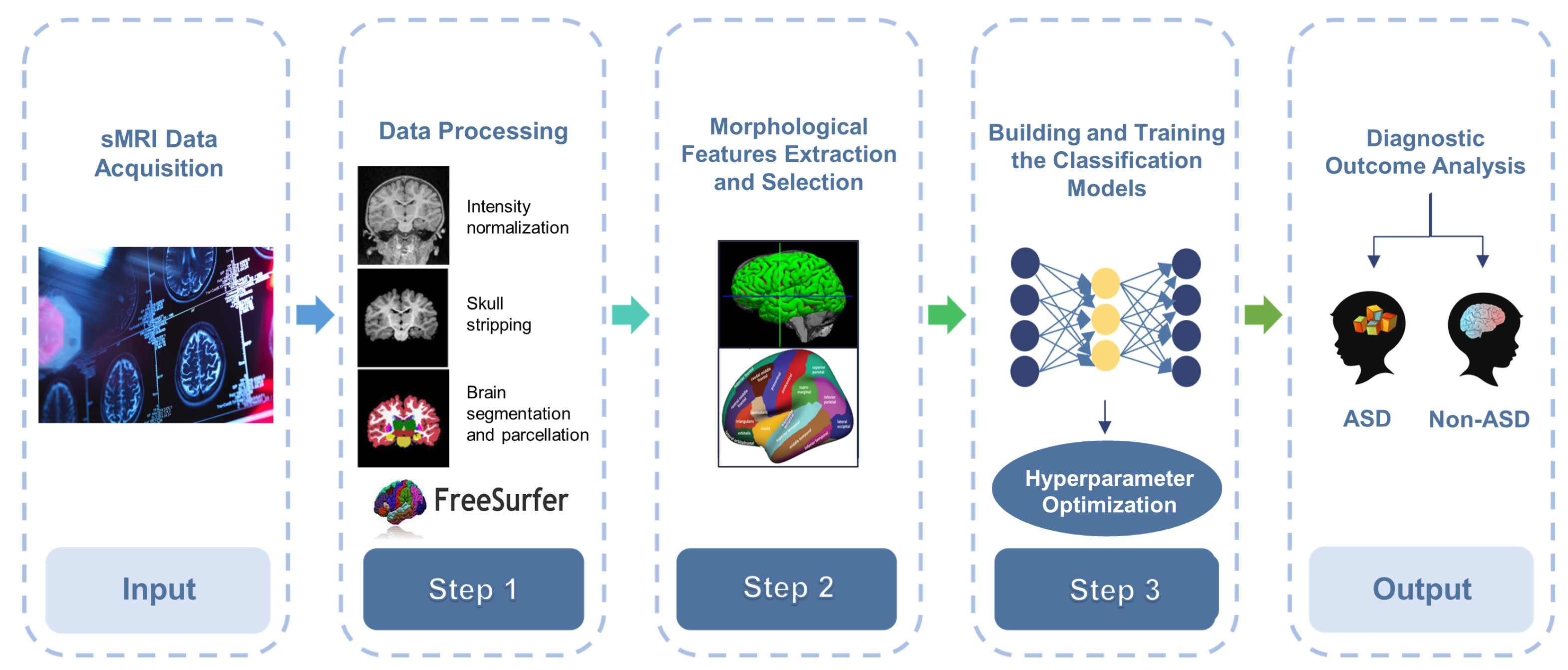
3. Methods and Materials

To ensure accurate and reliable predictions using multi-source and heterogeneous data, an ML-based system must address five primary challenges: data acquisition, data pre-processing, feature extraction and selection, model training, and model testing with performance evaluation. Our workflow for ASD classification, illustrated in Figure 2, outlines the steps involved, which will be elaborated in the subsequent subsections.

3.1. Data Acquisition

Three datasets were examined here: ABIDE I [32] and ABIDE II [33], which are publicly available datasets, and a local Saudi dataset. The ABIDE datasets include anonymized sMRI and rs-fMRI scans, along with personal, behavioral, and clinical diagnostic information collected from multiple sites stored in the ABIDE repository. Each study received ethical approval for data usage and sharing. We used 220 and 418 sMRI scans from ABIDE I and II, respectively. Detailed criteria for subject inclusion/exclusion and acquisition methodology can be found on the ABIDE website [34]. The data was downloaded usingCyberduck software v8.4.2 from an Amazon Web Services S3 container in the Neuroimaging Informatics Technology Initiative (NIFTI) file format [35], which is commonly used in image processing software. The data was organized according to the Brain Imaging Data Structure (BIDS) [36,37], facilitating script reuse and easy sharing between studies.

The KAU dataset comprised 33 participants who were recruited from KAU Hospital. A pediatric neurologist diagnosed the subjects with ASD based on DSM-5 criteria. None of the participants had ADHD, seizure disorder, or any other significant health problems. The control group (TD individuals) who had no notable health, neurological, or developmental problems. Participant scans were acquired in DICOM format using Siemens SKYRA or VERIO machines and then converted to NIFTI format using MRIcroGL v1.2.20220720 software [38,39]. A radiologist analyzed the MRI images visually to determine image quality, artifacts, and any gross abnormalities that needed to be excluded. The KAU Hospital Ethics Committee (approval number 386-21) approved the current study. All subjects in this work ranged from 5 to 10 years old to reduce the effect of dataset heterogeneity. T1-weighted sMRI scans were acquired in 3T scanners. Along with the sMRI data, general clinical information such as diagnosis (ASD or TD), age, and gender was collected for each participant. Investigating multiple datasets allows us to assess the robustness and generalizability of the proposed models. The demographic information of the studied participants is provided in

Table 2. Demographics of KAU, ABIDE I, and ABIDE II participants.

Dataset	ASD%	Male%	Age (years)	Total Participants
ABIDE I	47.7	82.7	6.4–10.9	220
ABIDE II	44.7	69.4	5.1–10.9	418
KAU	57.6	66.7	5.4–10.8	33

.

3.2. Pre-Processing

The acquired datasets were treated in six steps: image preprocessing and analysis, feature extraction, cleaning of the extracted data, transformation, splitting, and reduction.

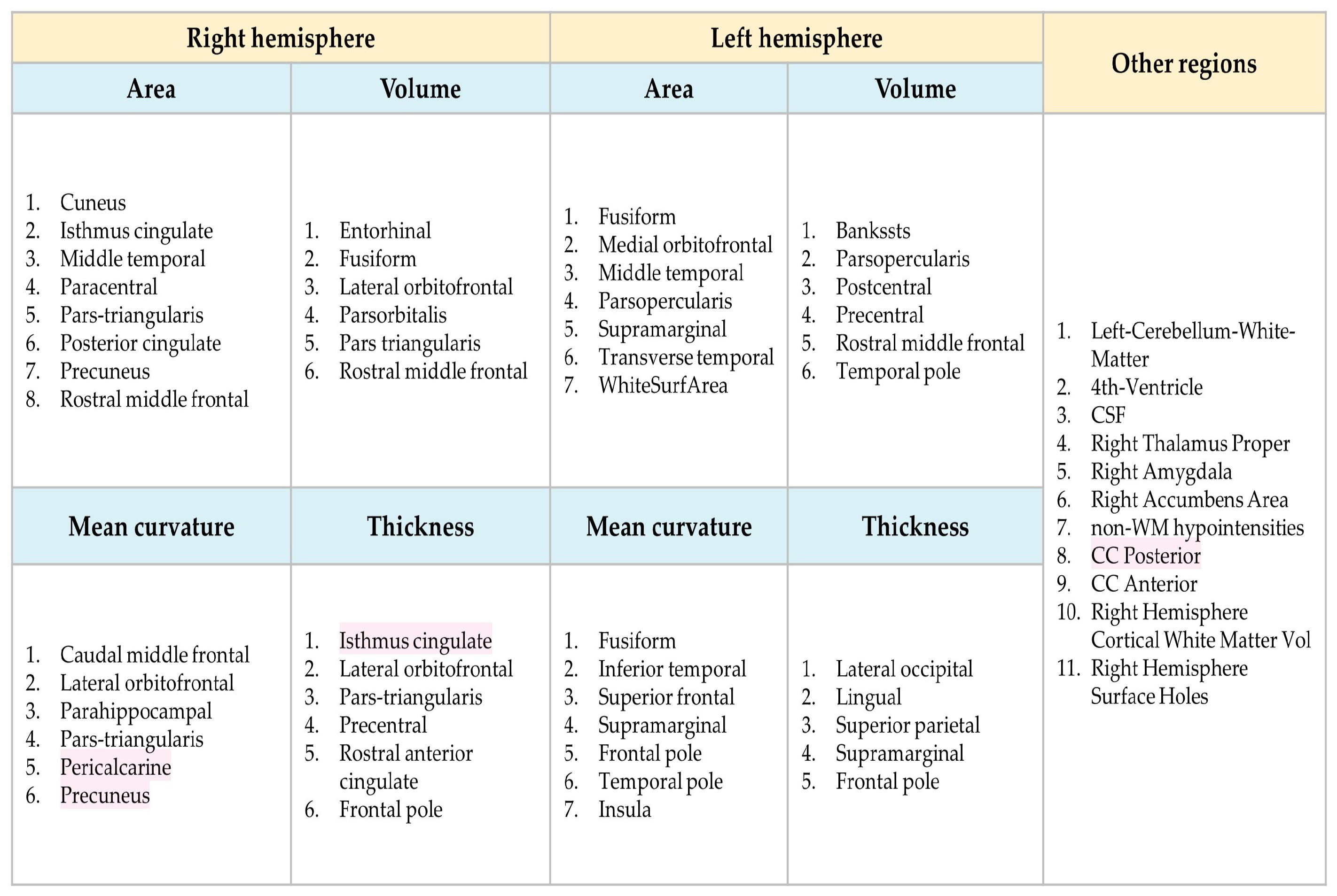
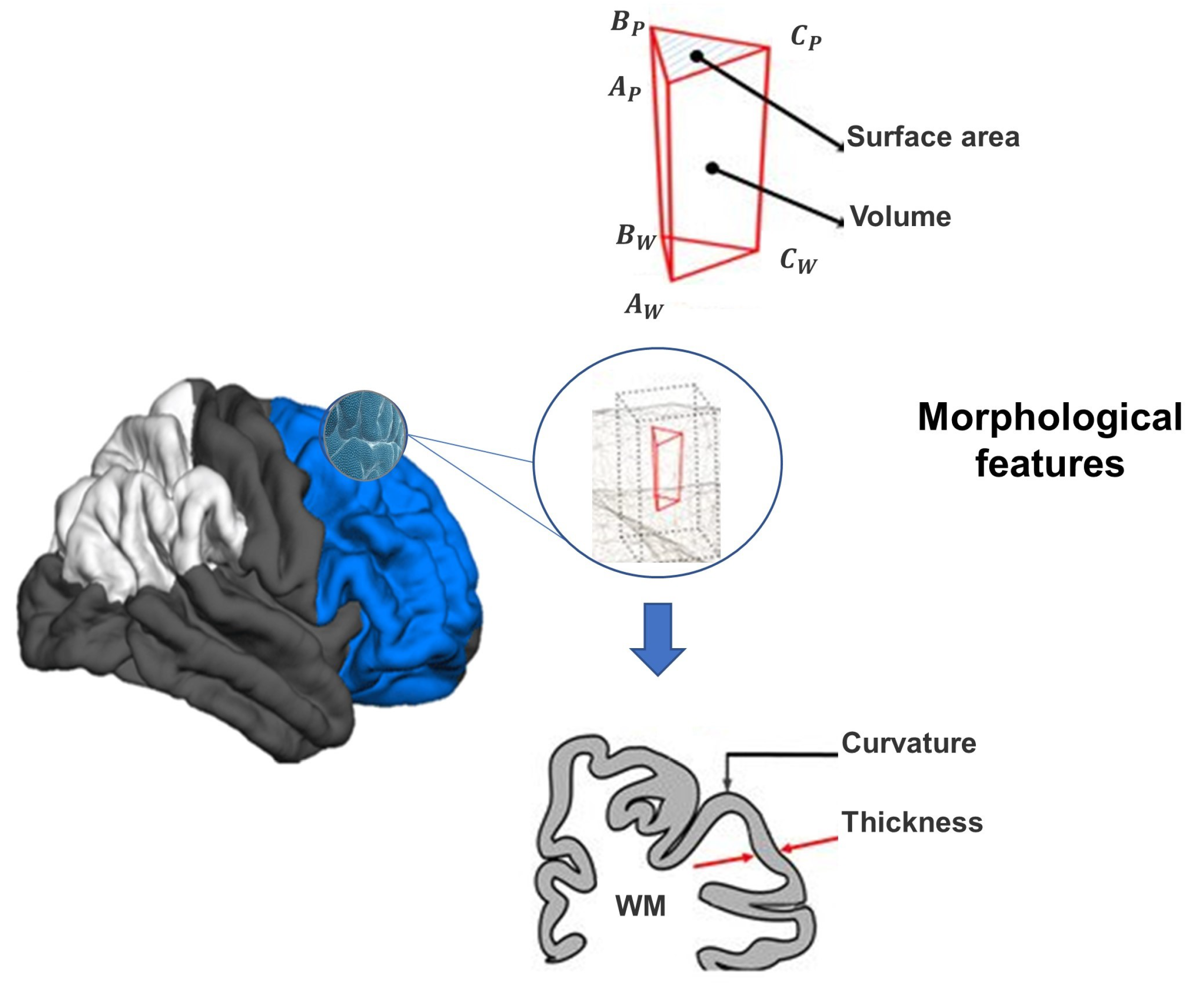
3.2.1. sMRI Pre-Processing and Features Extraction

For sMRI pre-processing and feature extraction, the well-known Recon-all pipeline from FreeSurfer V.5.3.0 software was employed. This pipeline addresses the challenges associated with developing and implementing pre-processing stages for neuroimaging data [40]. It improves the visual quality of the images, eliminates inter-subject variability caused by data gathering methods and artifacts, and enhances the reproducibility of the study [5,41]. Recon-all consists of 31 steps for surface-based analysis and volumetric segmentation, including intensity normalization, skull-stripping, brain segmentation, region labeling based on Desikan-Killiany (DK) atlas, surface amplification, spheroid atlas scoring, and cortical surface parcellation [40]. These steps are illustrated in Figure 3.

When executed on a personal computer, the Recon-all process generates substantial analytical volumes (approximately 400 MB) and takes around 10–20 h to complete. However, utilizing high-performance computers can significantly improve the performance of ML applications by efficiently managing large datasets and reducing computation time and resource demands [42]. To expedite the Recon-all pipeline, we utilized the Aziz Supercomputer, which allowed us to process data independently for each subject and in parallel, with 24 subjects using 24 CPUs. After completing all steps, the volume of subcortical structures (n = 66), surface area (SA) (n = 70), CTs (n = 70), mean curvatures (n = 68), and volumes (n = 68) of cortical structures were calculated. Descriptions of these morphological features can be found in

Table 3. List of the morphological regions of the Desikan-Killiany atlas.

Cortical Regions
#Label	Label Name	Name	#Label	Label Name	Name
1	lh bankssts	Banks of superior temporal sulcus	35	rh bankssts	Banks of superior temporal sulcus
2	lh caudal anteriorcingulate	Caudal anterior cingulate cortex	36	rh caudalanteriorcingulate	Caudal anterior cingulate cortex
3	lh caudal middlefrontal	Caudal middle frontal gyrus	37	rh caudal middlefrontal	Caudal middle frontal gyrus
4	lh cuneus	Cuneus	38	rh cuneus	Cuneus
5	lh entorhinal	Entorhinal cortex	39	rh entorhinal	Entorhinal cortex
6	lh fusiform	Fusiform gyrus	40	rh fusiform	Fusiform gyrus
7	lh inferiorparietal	Inferior parietal lobule	41	rh inferiorparietal	Inferior parietal lobule
8	lh inferiortemporal	Inferior temporal gyrus	42	rh inferiortemporal	Inferior temporal gyrus
9	lh lateraloccipital	Lateral occipital gyrus	43	rh lateraloccipital	Lateral occipital gyrus
10	lh caudal lateralorbitofrontal	Lateral orbitofrontal gyrus	44	rh caudal lateralorbitofrontal	Lateral orbitofrontal gyrus
11	lh lingual	Lingual gyrus	45	rh lingual	Lingual gyrus
12	lh caudal medialorbitofrontal	Medial orbitofrontal gyrus	46	rh caudal medialorbitofrontal	Medial orbitofrontal gyrus
13	lh middletemporal	Medial temporal gyrus	47	rh middletemporal	Medial temporal gyrus
14	lh parahippocampal	Parahippocampal gyrus	48	rh parahippocampal	Parahippocampal gyrus
15	lh paracentral	Paracentral gyrus	49	rh paracentral	Paracentral gyrus
16	lh parsopercularis	Pars opercularis	50	rh parsopercularis	Pars opercularis
17	lh parsorbitalis	Pars orbitalis	51	rh parsorbitalis	Pars orbitalis
18	lh parstriangularis	Pars triangularis	52	rh parstriangularis	Pars triangularis
19	lh pericalcarine	Pericalcarine gyrus	53	rh pericalcarine	Pericalcarine gyrus
20	lh postcentral	Postcentral gyrus	54	rh postcentral	Postcentral gyrus
21	lh posterior cingulate	Posterior cingulate cortex	55	rh posteriorcingulate	Posterior cingulate cortex
22	lh precentral	Precentral gyrus	56	rh precentral	Precentral gyrus
23	lh precuneus	Precuneus	57	rh precuneus	Precuneus
24	lh rostral anteriorcingulate	Rostral anterior cingulate cortex	58	rh rostral anteriorcingulate	Rostral anterior cingulate cortex
25	lh rostral middlefrontal	Rostral middle frontal gyrus	59	rh rostral middlefrontal	Rostral middle frontal gyrus
26	lh superiorfrontal	Superior frontal gyrus	60	rh superiorfrontal	Superior frontal gyrus
27	lh superiorparietal	Superior parietal gyrus	61	rh superiorparietal	Superior parietal gyrus
28	lh superiortemporal	Superior temporal gyrus	62	rh superiortemporal	Superior temporal gyrus
29	lh supramarginal	Supramarginal gyrus	63	rh supramarginal	Supramarginal gyrus
30	lh frontalpole	Frontal pole	64	rh frontalpole	Frontal pole
31	lh temporalpole	Temporal pole	65	rh temporalpole	Temporal pole
32	lh transversetemporal	Transverse temporal gyrus	66	rh transversetemporal	Transverse temporal gyrus
33	lh insula	Insula	67	rh insula	Insula
34	lh isthmuscingulate	Isthmus cingulate	68	rh isthmuscingulate	Isthmus cingulate
Sub-Cortical regions
69	Left Thalamus Proper	Thalamus	85	Right-Caudate	Caudate nucleus
70	Left-Hippocampus	Hippocampus	86	Right-Amygdala	Amygdala
71	Left-Caudate	Caudate nucleus	87	Right Accumbens area	Nucleus Accumbens
72	Left-Amygdala	Amygdala	88	Right-Lateral-Ventricle	Lateral ventricles
73	Left-Accumbens-area	Nucleus Accumbens	89	Right-Inf-Lat-Vent
74	Left-Lateral-Ventricle	Lateral ventricles	90	Right Cerebellum White Matter	Cerebellum-White-Matter
75	Left-Inf-Lat-Vent		91	Surfaces holes
76	Left-Cerebellum-White-Matter	Cerebellum-White-Matter	92	Right-Putamen	Putamen
77	Left-Putamen	Putamen	94	Right-choroid-plexus	Choroid-plexus
78	Left-Pallidum	Pallidum	95	Right-VentralDC	Ventral Diencephalon
79	Left-choroid-plexus	Choroid-plexus	96	Right-vessel	Vessel
80	Left-VentralDC	Ventral Diencephalon	97	3rd-Ventricle	Ventricle
81	Left-vessel	Vessel	98	4th-Ventricle
82	Right-Thalamus-Proper	Thalamus	99	5th-Ventricle
83	Right-Hippocampus	Hippocampus

and further elaborated in Table S1 in the Supplementary Materials. Furthermore, Figure S1 in the Supplementary Material represents the difference between cortical and subcortical regions in the DK atlas.

CT is the shortest distance between the WM and CSF boundaries per each vertex of the reconstructed cortical surface. Each vertex has a curvature for the pial surface and a curvature for the white surface. It demonstrates how curved each vertex is. It is calculated as the mean reciprocal of the principal radii. SA was designated as the GM/WM boundary. To calculate the cortical volume, multiply the SA by the CT [6,43]. Figure 4 visualizes the geometrical connection between CT, SA, and volume-derived measurements.

3.2.2. Data Cleaning and Integration

In traditional clinical diagnosis, clinicians often gather a wide range of personal and behavioral data, including factors such as ethnicity, or answers to question such as “Do ASD patients hear small sounds frequently while others do not?” [20]. Here, we utilized age and gender information, along with brain characteristics, as these variables were readily available in our datasets. However, it is important to note that real-world data is often inconsistent, noisy, and incomplete, which can pose challenges for ML systems. To address this, we performed a series of data cleaning operations. To handle missing values, we employed the SimpleImputer module, which estimates missing values by using the mean descriptive statistic for each column [44]. This approach helps to fill in the gaps and ensure that the data is more complete and suitable for analysis. Following data cleaning, we combined the ABIDE I and ABIDE II datasets into a single data repository.

Using the five measurements from Recon-all, we created various “features sets”. F1 represents a set of cortical region volumes, while F2, F3, F4, and F5 represent subcortical region volumes, SAs, CTs, and mean curvatures, respectively. The F6 set includes all measurements, for a total of 342 features.

3.2.3. Data Transformation

For ML model usage, we employed numeric transformation rules to encode the string feature “gender”. Female values were represented as 0, while male values were represented as 1. Additionally, to mitigate biases and ensure consistent modeling, we utilized standardization. This scaling technique independently rescaled each feature, centering the values around the mean with units of standard deviation [15].

3.3. Data Splitting

The combined features sets from the ABIDE datasets were randomly split into 80% for training and validation, and 20% for testing. To evaluate model performance and ensure stability, a 10-fold CV was conducted on the training and validation set. This involved dividing the data into 10 parts, with nine parts used for training and one part for validation, repeated 10 times.

The test set (KAU data) remained separate throughout the process, excluding it from training, model selection, and CV. Its sole purpose was to assess the model’s performance on unseen data. This separation ensured consistency, reduced heterogeneity within training datasets from different sources, and enabled unbiased evaluation in diverse contexts (such as different medical region or setting). Additionally, it allowed for an independent evaluation of the model’s adaptability on unique data characteristics. Analysis of local demographics may provide insights into the Saudi population, while utilizing a public database in the training and validation phases ensured standardized evaluation, facilitating comparisons with existing studies, knowledge, and benchmarks in the field.

Random_state was used to control randomization during data splitting [8].

3.4. Feature Selection

Compared to the number of instances, the feature extraction phase resulted in a large feature matrix (342 sMRI-based + age + gender). This ML challenge, known as the “dimensionality curse”, leads to overfitting, reduced performance, and increased memory and computational requirements. FS techniques address this issue by eliminating irrelevant, redundant, or noisy features while preserving the original data structure. This enhances classification accuracy, model interpretability, and mitigates overfitting [18].

Wrapper FS is based on a specific ML algorithm applied to a specific dataset. It compares all possible feature combinations using a search method to select the optimal features based on an evaluation criterion [45]. Specifically, we investigated RFECV, Boruta, and GWO-based wrapper techniques.

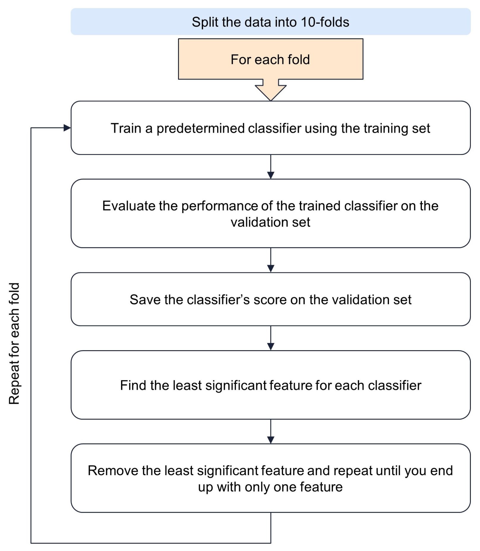
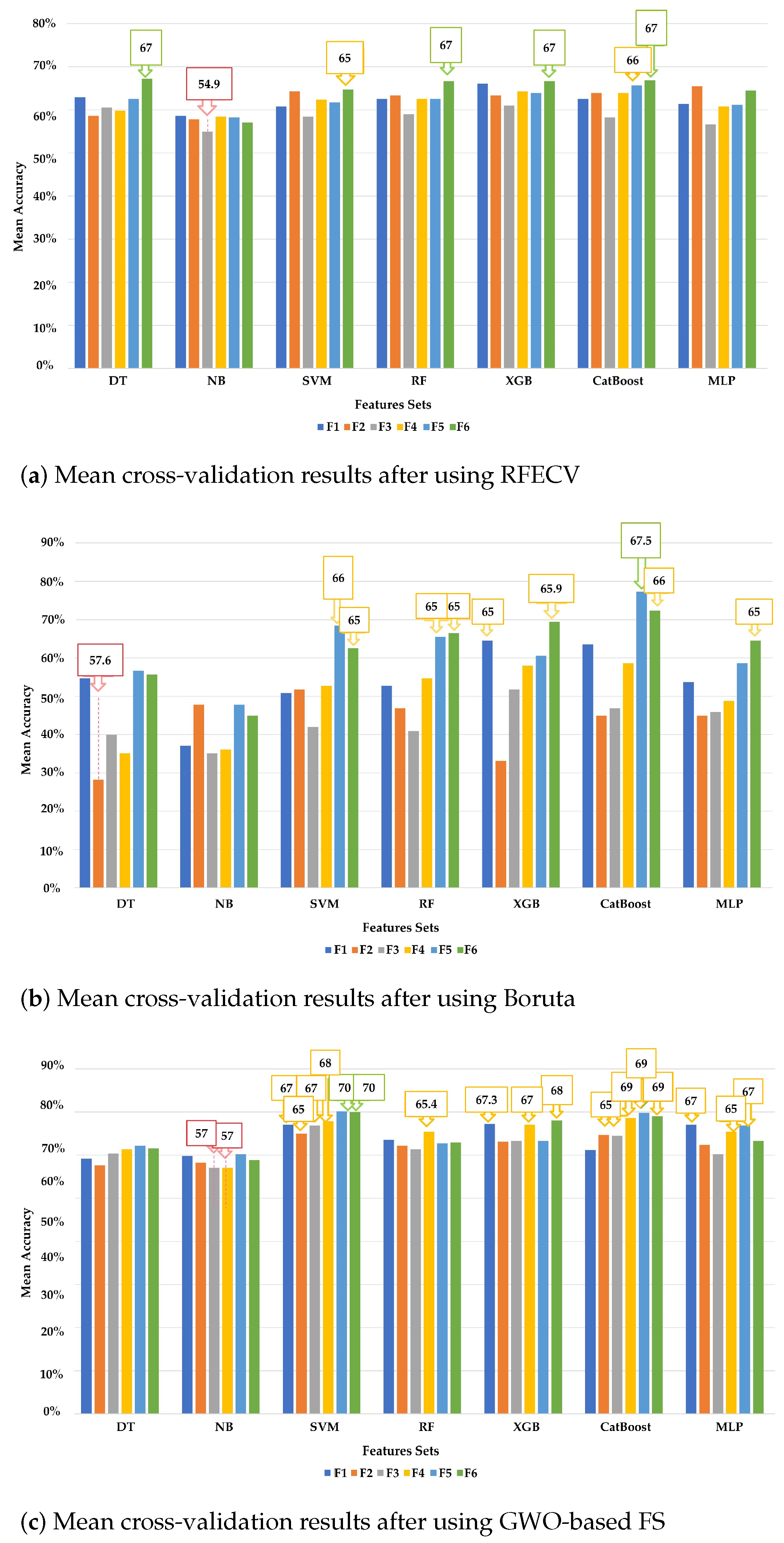
3.4.1. Recursive Feature Elimination with Cross-Validation (RFECV)

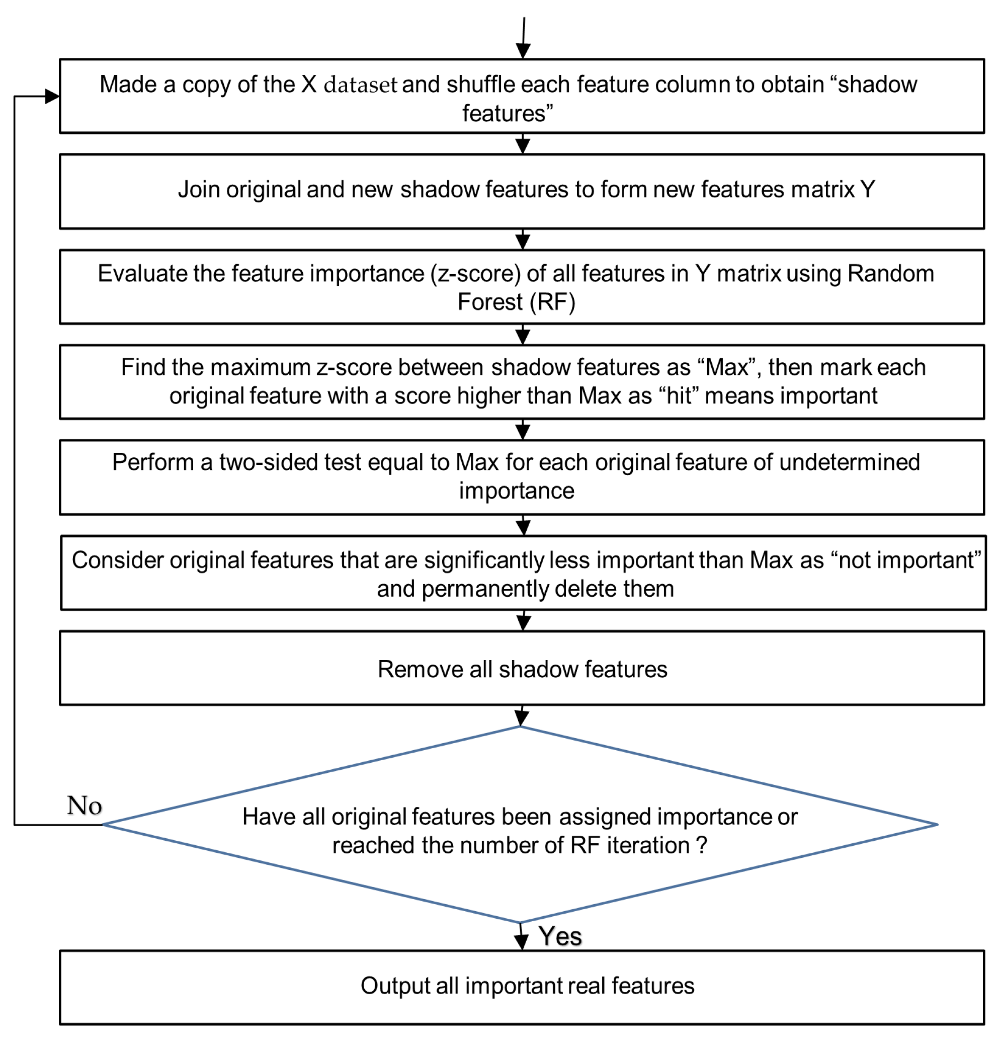
RFE, based on greedy optimization, iteratively eliminates features with weak relationships to the target variable (lowest importance) until reaching a predefined feature count. The sklearn RFECV module is an efficient RFE variant that explores the optimal feature subset by for a given estimator (by default DT) removing 0 to N features using RFE and evaluating the model’s 10-fold CV score. The resource requirements may vary based on data size and the chosen estimator [46,47]. Figure 5 shows the RFECV algorithm flowchart.

3.4.2. Boruta

Boruta, an R algorithm, has been ported to Python as the BorutaPy library [48]. The flowchart of Boruta is illustrated in Figure 6.

Boruta operates based on two principles: shadow features and binomial distributions. Initially, it creates “shadow features” by duplicating and shuffling the columns of the original dataset. These shadows are then combined with the original features to create a new dataset. A RF model is trained on this new dataset, and the feature importance is determined iteratively using the “Z value”, which measures the mean accuracy reduction. Higher Z values indicate more significant features. When a feature’s importance surpasses a predefined threshold, it is considered a “hit”. However, to avoid discarding potentially useful features due to chance, Boruta employs a binomial distribution approach. By repeating the process considering the binary outcomes of “hit” or “not hit” for each feature, Boruta determines which features should be retained and which should be discarded [49].

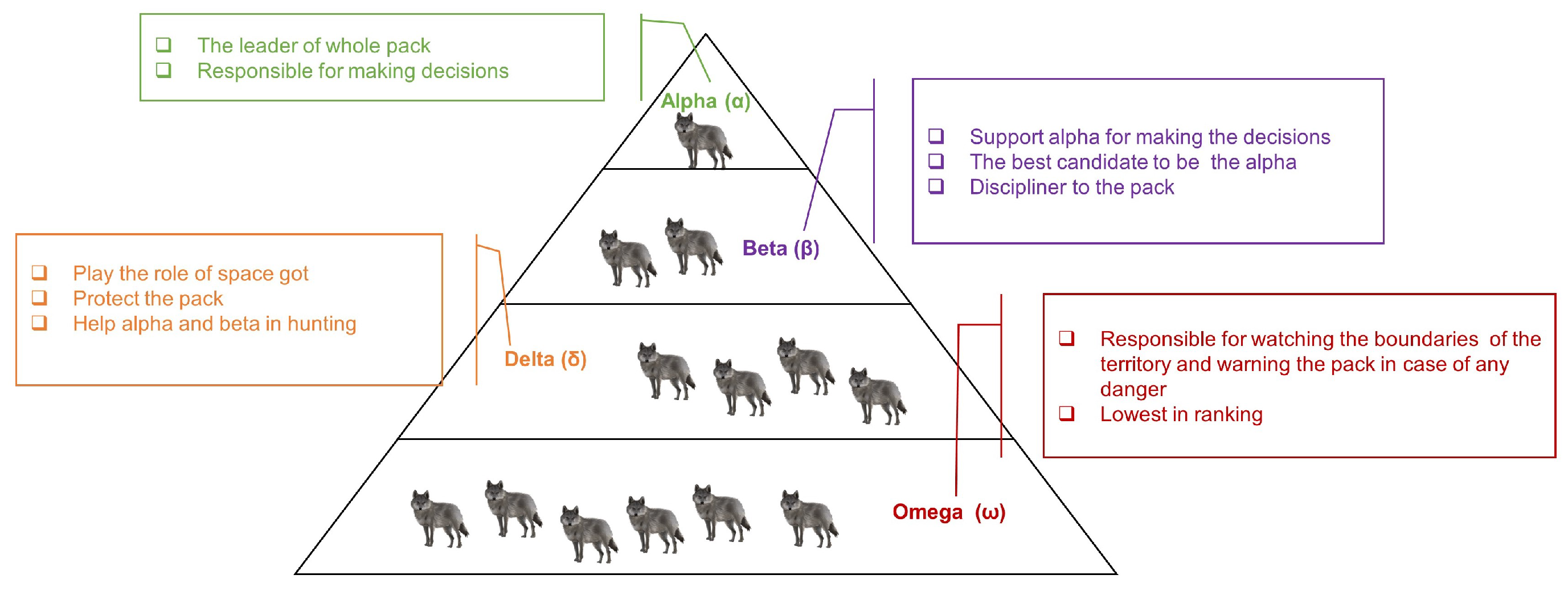
3.4.3. Grey Wolf Optimizer (GWO)-Based Algorithm

GWO is a bio-inspired meta-heuristic algorithm based on the social behavior of grey wolves, known for their hierarchical pack structure [50]. Figure 7 illustrates this hierarchical structure.

Here, we utilized the GWO object from the Niapy library [51]. The GWO algorithm utilizes alpha ($\alpha$), beta ($\beta$), delta ($\delta$), and omega ($\omega$) wolves to find the optimal solution. Each wolf represents a potential solution, with the alpha wolf making major decisions. The beta ($\beta$) wolf aids the $\alpha$ wolf in decision making and enforces the alpha wolf’s leadership among the lower-ranked wolves. Delta ($\delta$) are senior wolves or sentinels who protect the $\alpha$ and $\beta$ and control the omega $\omega$ wolves. Wolves’ positions are updated based on prey location and a fitness function. The best solutions are ranked as $\alpha$, $\beta$, and $\delta$ according to fitness. Omega wolves’ positions are adjusted based on the top three wolves positions, denoted as ${\overrightarrow{X}}_{\alpha }$, ${\overrightarrow{X}}_{\beta }$, and ${\overrightarrow{X}}_{\delta }$. Prey encircling, hunting, attacking, and searching are key steps in the algorithm and are mathematically represented as follows:

• Initialize the positions of the wolves randomly within the search space.
• Prey Encircling: update the positions of the wolves based on the alpha wolf’s position, aiming to encircle the prey. The position of each wolf is updated using the following equation: ${\overrightarrow{X}}_i={\overrightarrow{X}}_{\alpha }-\overrightarrow{A}\times {\overrightarrow{C}}_i$, where ${\overrightarrow{X}}_i$ is the position of the ith wolf, ${\overrightarrow{X}}_{\alpha }$ is the position of the alpha wolf, $\overrightarrow{A}$ is a random vector, and ${\overrightarrow{C}}_i$ is a coefficient vector.
• Prey Attacking: update the positions of the wolves to attack the prey. The position of each wolf is updated using the following equation: ${\overrightarrow{X}}_i={\overrightarrow{X}}_p-\overrightarrow{A}\times {\overrightarrow{C}}_i$, where ${\overrightarrow{X}}_p$ is the position of the prey.
• Searching: update the positions of the wolves to search for the prey. The position of each wolf is updated using the following equation: ${\overrightarrow{X}}_i={\overrightarrow{X}}_i+\overrightarrow{A}\times {\overrightarrow{C}}_i$, where $\overrightarrow{A}$ is a random vector, and ${\overrightarrow{C}}_i$ is a coefficient vector.
• Boundary Checking: ensure that the updated positions of the wolves remain within the defined search space.
• Fitness Evaluation: evaluate the fitness of each wolf based on the problem-specific fitness function.
• Select the three wolves with the best fitness values as the alpha, beta, and delta wolves, respectively.
• Update the positions of the omega wolves based on the positions of the alpha, beta, and delta wolves.
• Termination: repeat steps 2–8 until a termination criterion is met (e.g., a maximum number of iterations or a desired fitness value is reached).

The GWO algorithm flowchart represented in Figure 8.

3.5. Models Development and Training

The work utilizes seven ML algorithms for distinguishing between ASD and TD individuals. Here is a brief description of each algorithm:

3.5.1. Machine Learning (ML) Algorithms

• Support vector machine (SVM):
  SVM finds an optimal decision boundary (hyperplane) in a high-dimensional space to separate different classes. It maximizes the margin between classes and can handle non-linear classification using kernel methods. SVM is suitable for handling high-dimensional data such as sMRI, but training time can be long [5].
• Naïve Bayes (NB):
  NB is based on Bayes’ theorem and assumes that features are independent and contribute independently to the final prediction. Gaussian NB, which follows the normal distribution, is used in this work. NB is known for its simplicity and efficiency, and it is particularly useful when dealing with large datasets [52,53].
• Decision Tree (DT):
  DT is a flowchart-like tree structure that represents a series of decisions and their outcomes. Starting from a root node, it uses a top-down greedy search to produce a DT with decision and leaf nodes without backtracking over the space of possible branches. The DT branches describe the dataset’s features. The final classification is made at the leaf nodes of the tree. DTs are intuitive and easy to interpret, but they can be prone to overfitting [54].
• Random Forest (RF):
  RF is an ensemble learning method that combines multiple weak learners (e.g., DTs) to create a robust model. Each tree is trained on a random subset of the original dataset using a bagging technique. The final prediction is determined by majority voting. RF improves performance and reduces overfitting compared to a single DT [17].
• Extreme Gradient Boosting (XGB):
  XGB is an optimized version of the GBC algorithm. It is designed for speed and performance, utilizing three techniques: implementation of sparse-aware that handles missing data values automatically; utilization of a block structure to facilitate the parallelization of tree construction; and continuous training to further enhance the model’s performance that has been fitted to new data [14,55].
• Category Boosting (CatBoost):
  CatBoost is a gradient boosting approach that specifically works well with categorical features. It creates a set of DTs with identical splitting criteria throughout the entire level. Each successive tree is produced with a lower loss than the previous one. CatBoost is well-balanced and less sensitive to overfitting [55].
• Multilayer perceptron (MLP):
  MLP is an artificial neural network with input, output, and hidden layers. The input layer receives the data represented by a digital vector to be processed. Classification is handled by the output layer. A number of hidden layers make up the MLP’s true computational engine. MLP processes input data through linear and nonlinear transformations, transmitting the data forward. The network learns from feedback on prediction errors through the backpropagation learning process, adjusting weights for improved predictions [56].

3.5.2. Hyperparameter Optimization

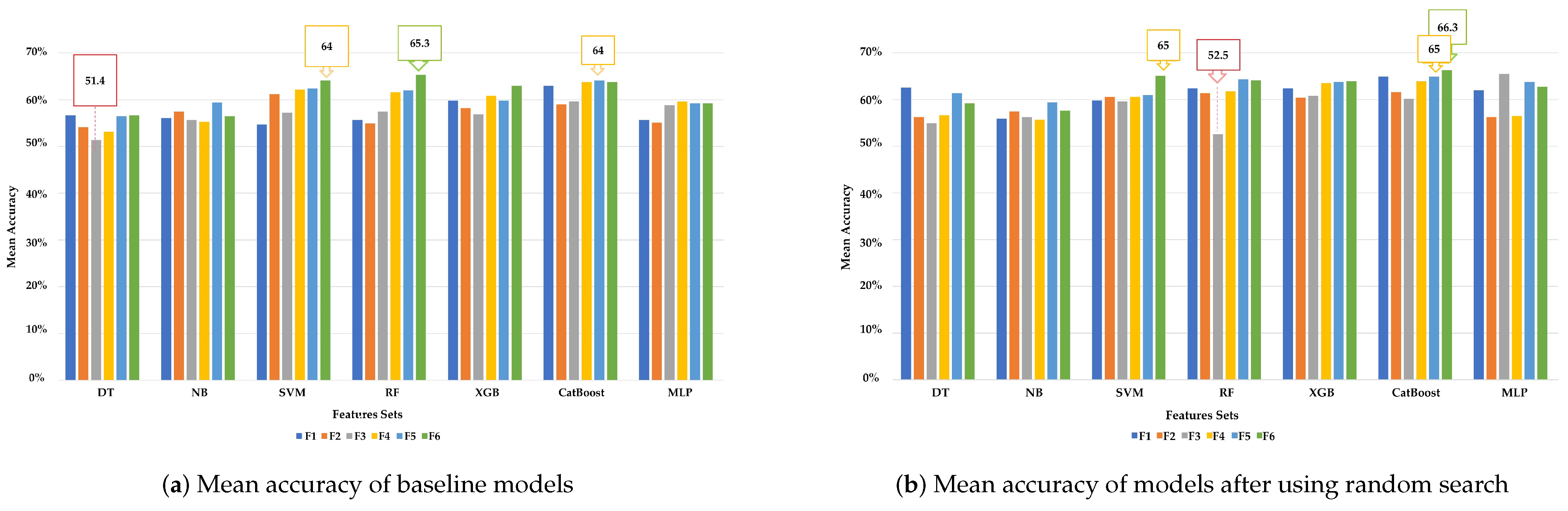
Hyperparameter optimization is vital for achieving optimal performance in ML algorithms. It involves adjusting the algorithm’s hyperparameters during training to best fit the dataset. Grid search and random search are commonly used methods for tuning hyperparameter values. Recently, population-based algorithms like GWO have gained popularity for hyperparameter optimization [57]. In this study, we examined random search and GWO with a 10-fold cross-validation (CV).

• Random Search:
  Random search explores a specified number of random hyperparameter combinations. It is faster than grid search but does not guarantee finding the optimal combination. Here, the RandomizedSearchCV function from sklearn was used with 20 iterations to find the best hyperparameters [58].
• GWO-based hyperparameters tuning:
  GWO is a nature-inspired algorithm. It is faster and more likely to find the best solution compared to random search. The GWO algorithm was used for hyperparameter tuning with the NatureInspiredSearchCV function from the sklearn_nature_inspired_algorithms library. Parameters such as the model name, population size and maximum stagnating generation were set for the optimization process [57,59]. Here, the population size is set to 50 and the max stagnating generation is 20.

Different hyperparameter combinations were searched using random and GWO-based search algorithms, and the values yielding the highest model accuracy on the validation set were selected. For a comprehensive list of hyperparameters, refer to

Table 4. The different values of models’ hyperparameters used in our study.

Model Name	Hyperparameter Name	Definition	Hyperparameter Value Range
Support Vector Machine (SVM)	C value	The penalty parameter	(0.1, 0.8, 0.9, 1, 1.1, 1.2, 1.3, 1.4, 0.25, 0.5, 0.75, 10, 100)
	Kernel	Defining the algorithm	linear, rbf, poly, and sigmoid
	Degree	The degree of the polynomial kernel function (‘poly’)	1, 2, 3, 4, 5, 6
	Gamma	Kernel coefficient	scale, auto
Decision Tree (DT)	Criterion	The function to measure the quality of a split	Gini and entropy
	Max_depth	The maximum depth of the tree	None, 2, 4, 6, 8, 10, or 12
Random forest (RF)	N_estimators	Number of estimators	10, 20, 50, 64, 100, 140, 200, and 256
	Min_samples split	Minimal sample count necessary to split an internal node	1, 2, 3, 6
	Min_samples_leaf	Minimum amount of samples at the tree’s leaves	1, 6, and 10
	Max_features	The number of features to consider for the best split	sqrt, log2, None
	Criterion of trees	The function to measure the quality of a split	Gini and entropy
	Max depth	The maximum depth of the tree	None, 2, 4, 5, 6, 7, 8, 16, or 30
Naïve Bayes (NB)	Smoothing	Laplace smoothing technique helps tackle the problem of zero probability	($1\times {10}^{-1}$, $1\times {10}^{-2}$, $1\times {10}^{-3}$, $1\times {10}^{-4}$, $1\times {10}^{-5}$, $1\times {10}^{-6}$, $1\times {10}^{-7}$, $1\times {10}^{-8}$, $1\times {10}^{-9}$ )
Extreme Gradient Boosting (XGB)	Max depth	Maximum depth of the individual estimators/trees	3, 4, 5, 6, 8, 10, 12, 15
	Gamma	Minimum loss reduction required to partition a leaf node of the tree	0, 0.1, 0.2, 0.3, 0.4
	Colsample by tree	subsample ratio of columns when constructing each tree	0.3, 0.4, 0.5, 0.7, 1
	Learning rate	Step size shrinkage used in update to prevents overfitting	0.05, 0.10, 0.15, 0.20, 0.25, 0.3
	Min child weight	Minimum sum of instance weight needed in a child	1, 3, 5, 7
Category Boosting (CatBoost)	Depth	Depth of the tree	1, 2, 3, 4, 5, 6, 7, 8, 9, 10
	Learning rate	The rate at which the model weights are updated after working through each batch of training examples	0.01, 0.02, 0.03, 0.04, 0.009
	Iteration	The maximum number of trees that can be built	10, 20, 30, 40, 50, 60, 70, 80, 90, 100, 250, 500
Multi-layer Perceptron (MLP)	Hidden layer sizes	Number of hidden layers	(50,50,50), (50,100,50), (100), (10,30,10), (100, 3), (3,3), and (20)
	Activation	Activation function for the hidden layer	‘identity’, ‘logistic’, ‘tanh’, or ‘relu’.
	Solver	The solver for weight optimization	‘lbfgs’, ‘sgd’, or ‘adam’
	Alpha	Strength of the L2 regularization term	0.0001, $1\times {10}^{-5}$, and 0.05
	Learning rate	Learning rate schedule for weight updates	‘constant’, ‘invscaling’, ‘adaptive’

.

3.6. Model Testing and Performance Evaluation

K-fold CV is a commonly used technique to evaluate algorithm performance and optimize hyperparameters. The dataset is divided into k subsets, with one subset used as the validation set and the remaining subsets as the training dataset. This process is repeated k times, ensuring that each subset serves as the validation set once.

In many studies, the value of k set to 10 strikes a balance between comprehensive testing, computational efficiency, and unbiased estimation of model performance. By using K-fold CV, a more robust assessment of the algorithm’s general performance can be obtained compared to using a single train-test split or different values of k [11].

To evaluate the performance of our models, we employed three metrics: accuracy, sensitivity (Sen), and specificity (Spe). In binary classification tasks, sensitivity (also known as the true positive rate) measures the proportion of positive instances correctly identified, specifically the percentage of individuals with ASD who are accurately classified as having the disorder. On the other hand, specificity (also known as the true negative rate) quantifies the proportion of negative instances correctly identified, representing the percentage of TD individuals correctly classified as not having the disorder. Accuracy, the third metric, indicates the overall percentage of correctly classified instances across all classes [5].

4. Results and Discussion

4.1. Result Analysis

Three experiments were conducted using Python v3.11 and Jupyter Notebook v6.4.5, as described in Section 3.

4.1.1. Experiment 1 Results

Experiment 1 assessed the feasibility of using brain morphological features for classifying ASD and TD individuals. Two sub-experiments were conducted using 80% of the ABIDE dataset, employing the 10-fold CV technique with or without random search for hyperparameter tuning. The experimental results, presented in Figure 9, enable a comparison of the performance of the tested models based on the extracted descriptors.

The accuracy of ASD classification varied across different algorithms and features sets. However, upon analyzing the above figure, it is clear that the baseline models did not consistently perform well across all feature sets. The mean accuracy values ranged from 51.4% to 65.3%, depending on the feature set. The DT model in the F3 group had the lowest mean accuracy, while the RF model in the F6 group, which incorporated 342 biomarkers/features from all brain regions, achieved the highest mean accuracy.

Table 5. Experiment 1: performance results of the best baseline models (according to average cross-validation accuracy) for each feature set.

Experiment 1.1: Baseline Models
Model	Feature Set/Number of Features	Model Performance on Training Dataset	Prediction Performance on Testing Dataset
		Mean Accuracy	ABIDE I + ABIDE II			KAU
			Accuracy	Sensitivity	Specificity	Accuracy	Sensitivity	Specificity
CatBoost	F1: cortical region’s volumes/66	62.94	58.81	57.81	56.76	63.64	63.64	61.84
SVM	F2: volumes of sub-cortical regions/68	61.18	61.94	60.94	60.46	69.7	69.7	67.11
CatBoost	F3: surface area of sub-cortical regions/70	59.61	62.72	61.72	60.39	54.55	54.55	53.01
CatBoost	F4: cortical thickness of sub-cortical regions/70	63.73	61.16	60.16	58.03	72.73	72.73	67.86
CatBoost	F5: mean curvatures of sub-cortical regions/68	64.12	69.75	68.75	67.47	63.64	63.64	62.78
RF	F6: all features/342	65.29	65.84	62.5	61.56	48.48	48.48	44.92

presents the performance results of the best baseline model in terms of average CV accuracy among the seven models studied for classifying ASD based on different brain feature sets.

Based on the results presented in Table 5, it is evident that the CatBoost model consistently outperforms the other models across most feature sets. The SVM and RF models also demonstrate good performance.

The random search process for hyperparameter tuning was limited to 20 iterations, as further improvements were not expected beyond that point. In each iteration, hyperparameters were tuned, and performance analysis was conducted to identify the parameters with the best performance.

Figure 9 indicates improved performance for most models after hyperparameter tuning. The RF model with F3 achieved the lowest accuracy (52.55%), while CatBoost with F6 achieved the highest accuracy (66.28%). The best hyperparameters were a learning rate of 0.02, 60 iterations, and a depth of 6.

Table 6. Experiment 1: performance results of the best baseline models (according to average cross-validation accuracy) for each feature set after using the random search technique.

Experiment 1.2 : Models with Random Search
Model	Feature Set /Number of Features	Model Performance on Training Dataset	Prediction Performance on Testing Dataset
		Mean Accuracy	ABIDE I + ABIDE II			KAU
			Accuracy	Sensitivity	Specificity	Accuracy	Sensitivity	Specificity
CatBoost	F1: cortical region’s volumes/66	64.91	59.59	58.59	57.68	78.79	78.79	78.76
CatBoost	F2: volumes of sub-cortical regions/68	61.57	64.28	63.28	61.99	72.73	72.73	71.62
XGB	F3: surface area of sub-cortical regions/70	60.78	59.59	58.59	58.68	57.58	57.58	55.64
XGB	F4: cortical thickness of sub-cortical regions/70	63.53	60.38	59.38	58.95	66.67	66.67	63.53
CatBoost		63.92	62.72	61.72	58.91	84.85	84.85	82.14
CatBoost	F5: mean curvatures of sub-cortical regions/68	64.91	69.75	68.75	66.72	72.73	72.73	73.50
CatBoost	F6: all features/342	66.27	65.84	64.84	63.09	51.5	48.49	44.92

presents the results of the best model for each feature set. CatBoost demonstrates excellence once again, and XGB also exhibits good performance.

4.1.2. Experiment 2 Results

Experiment 2 aimed to assess the impact of three different FS techniques: RFECV, Boruta, and a GWO-based algorithm on the overall performance of the models. Each technique was evaluated individually to determine its effectiveness.

RFECV and Boruta were applied after the random search hyperparameter tuning algorithm. This approach enabled the selection of optimal hyperparameters while considering the FS process.

On the other hand, the GWO-based algorithm encompassed both hyperparameter tuning and FS within a unified optimization framework, combining both aspects in separate steps.

The results of Experiment 2 can be seen in Figure 10.

In Experiment 2, RFECV resulted in mean validation accuracies ranging from 54.90% to 67.28%. The best accuracy (67.28%) was achieved by the DT model with 16 features from the F6 set (learning rate = 0.04, iterations = 250, depth = 6). On the ABIDE test dataset, the DT model achieved 61.2% accuracy, while on the KAU data it achieved 45.5%. The lowest classification accuracy was obtained by NB with the F3 set.

In the Boruta sub-experiment, CatBoost with the F5 set achieved the highest accuracy (67.5%), while DT with the F2 set had the lowest accuracy (57.65%). CatBoost selected only four left-brain features as the most important, with a learning rate of 0.03, 100 iterations, and a maximum depth of 10. On the ABIDE and KAU test datasets, CatBoost achieved accuracies of 62.7% and 72.7%, respectively.

In the GWO-based sub-experiment, the mean validation accuracies ranged from 57.06% to 70.20%. The highest accuracy was achieved by SVM with 11 features from the F5 set (70%) and 62 features from the F6 set. The lowest accuracies were obtained by NB with 14 features from the F3 set and NB with 19 features from the F4 set. On the ABIDE test set, SVM achieved an accuracy of 65.8% with the F6 set and 63.5% with the F5 set. On the KAU test set, SVM achieved an accuracy of 57.6% with the F6 set and 69.7% with the F5 set.

Table 7. Experiment 2: performance results of the best optimized models (according to average cross-validation accuracy) for each feature set after using feature selection algorithms.

Model	Feature Set/Number of Features	Model Performance on Training Dataset	Prediction Performance on Testing Dataset
		Mean Accuracy	ABIDE I + ABIDE II			KAU
			Accuracy	Sensitivity	Specificity	Accuracy	Sensitivity	Specificity
Experiment 2.1: models with random search and recursive feature elimination with cross-validation (RFECV)
XGB	F1: cortical region’s volumes/12	66.08	59.59	58.59	57.43	63.64	63.64	63.72
MLP	F2: volumes of sub-cortical regions/17	65.49	64.28	63.28	61.74	69.7	69.7	67.11
DT	F3: surface area of sub-cortical regions/16	60.59	58.81	57.81	59.01	66.67	66.67	63.53
XGB		60.98	55.69	54.69	53.05	57.58	57.58	57.52
XGB	F4: cortical thickness of sub-cortical regions/19	64.31	61.94	60.94	58.67	66.67	66.67	62.59
CatBoost	F5: mean curvatures of sub-cortical regions/29	65.69	65.84	64.84	62.84	69.7	69.7	68.05
DT	F6: all features/342	67.24	61.16	60.16	59.03	45.45	45.45	41.35
Experiment 2.2: models with random search and Boruta
XGB	F1: cortical region’s volumes/6	64.90	54.91	53.91	51.88	60.61	60.61	63.91
CatBoost		64.71	61.94	60.94	60.21	66.67	66.67	60.71
SVM	F2: volumes of sub-cortical regions/4	62.35	65.84	64.84	63.84	66.67	66.67	67.29
XGB	F3: surface area of sub-cortical regions/3	62.35	56.47	56.48	54.98	48.48	48.48	48.68
XGB	F4: cortical thickness of sub-cortical regions / 4	63.53	58.81	57.81	57.3	57.58	57.58	54.7
CatBoost		63.73	58.81	57.81	56.91	66.67	66.67	61.65
CatBoost	F5: mean curvatures of sub-cortical regions/4	67.45	62.72	61.72	60.14	72.73	72.73	72.56
NB	F6: all features/8	70.13	65.84	64.84	60.01	60.61	60.61	55.45
SVM		70.08	60.38	59.38	56.86	54.55	54.55	52.08
RF		70.05	58.03	57.03	55.09	66.67	51.52	52.26
Experiment 2.3: models with random search and grey wolf-based optimizer (GWO)
SVM	F1: cortical region’s volumes/16	67.06	61.94	60.94	59.46	54.55	54.55	49.25
XGB		67.25	55.69	54.69	53.80	60.61	60.61	58.27
MLP		67.06	59.59	58.59	57.18	60.61	60.61	56.39
SVM	F2: volumes of sub-cortical regions/19	65	60.38	59.38	57.86	57.86	57.58	56.58
SVM	F3: surface area of sub-cortical regions/14	66.86	55.69	54.69	53.30	54.55	54.55	51.13
XGB	F4: cortical thickness of sub-cortical regions/19	63.53	60.38	59.38	58.95	66.67	66.67	63.53
CatBoost		68.63	61.16	60.16	58.03	66.67	66.67	62.59
SVM	F5: mean curvatures of sub-cortical regions/11	70	63.5	62.5	60.31	69.7	69.7	67.12
SVM	F6: all features/62	70	65.84	64.84	63.34	57.58	57.58	54.69

displays the results of the best-performing model, determined by mean accuracy, for each feature set in the optimization experiments.

Across these three experiments, the SVM model consistently demonstrated good performance, followed by the ensemble models CatBoost and XGB, particularly when using the F5 and F6 feature sets. On the other hand, the F3 feature set consistently resulted in the worst performance. Notably, NB and DT classifiers consistently had the lowest mean validation accuracy, which may be attributed to their assumption of equal statistical relevance among features.

4.1.3. Experiment 3 Results

In the final experiment, the optimal brain features identified in the top three models from Experiment 2 were combined with age and gender features. The hyperparameters of these models were then tuned using the GWO-based hyperparameter optimization algorithm. To assess the potential improvement in ASD classification, these models were re-evaluated using a 10-fold CV scheme, and their mean validation accuracy was measured.

Figure 11 and

Table 8. Experiment 3: performance results of the best optimized models (according to average cross-validation accuracy) that use selected features from the brain combined with age and gender information.

Experiment 3: Models with GWO-Based Hyperparameter Tuning and Feature Selection Algorithms + Age and Gender
Model	Feature Set/Number of Features	Model Performance on Training Dataset	Prediction Performance on Testing Dataset
		Mean Accuracy	ABIDE I + ABIDE II			KAU
			Accuracy	Sensitivity	Specificity	Accuracy	Sensitivity	Specificity
SVM		70.19	63.5	62.5	60.31	69.67	69.67	67.12
XGB	F5: mean curvatures of sub-cortical regions/13	67.06	58.03	57.03	55.33	78.79	78.79	75
CatBoost		69.80	62.72	61.72	60.14	63.64	69.7	66.17
SVM	F6: all features/62	71	64.28	63.28	61.74	57.58	57.58	53.76
XGB		68.63	59.59	58.59	57.18	45.45	45.45	43.23
CatBoost		69.02	62.72	61.72	60.14	52.51	51.52	50.38

showcase the results of the three models, ranked by mean accuracy, in the third experiment.

In this experiment, the mean validation accuracy values ranged from 67.06% to 71%. The SVM model achieved the highest accuracy with 62 features from the F6 set, while the XGB model achieved the lowest accuracy with 13 features from the F5 set.

According to the table, under the 10-fold CV scheme, the SVM model with the F6 set demonstrated an improvement in performance, increasing from 70% in Experiment 2 to 71% in this experiment. This accuracy represents the highest achieved thus far. However, the test accuracy on the test datasets remained unchanged. The best-performing SVM model on the F6 test set from ABIDE achieved an accuracy of 64.28%, while on the KAU test set it achieved an accuracy of 57.58%. The hyperparameters for this model were set as C = 1, kernel = ‘rbf’, and gamma = 0.01. Detailed performance measures for all models in all experiments can be found in the Supplementary Materials (Tables S2–S5).

4.2. Discussion

This study explored ASD classification using seven models based on morphological features from various sMRI datasets of children aged 5–10 years. Different algorithms applied to the same data yielded a wide range of classification results.

The baseline models demonstrated limited reliability and accuracy. However, the performance of tuned models improved, with a mean accuracy ranging from 52.55% to 66.28%. Notably, certain classifiers, such as NB and MLP, did not perform well, potentially due to insufficient training data relative to the number of dimensions, as well as variations arising from data sources, imaging techniques, and participant characteristics.

Additionally, grid search exhaustively explores all combinations of hyperparameter values but is computationally expensive, while random search tries a subset of values to adjust the models [60]. However, both methods lack informative selection. In the recent experiment, nature-based methods efficiently searched for optimal hyperparameter values. The informative GWO algorithm, applied here for the first time in ASD studies, shows promise for future researchers to explore other sophisticated algorithms and enhance classification accuracy.

The primary objective of this paper is not only to improve the accuracy of ASD classification but also to investigate the structural evidence associated with ASD. Recognizing that not all features carry equal importance, each feature contributes to the overall ASD classification score. In Experiment 2, various FS techniques, including RFECV, Boruta, and GWO-based algorithms, were employed to enhance model accuracy by reducing complexity, avoiding overfitting, and addressing the curse of dimensionality.

Previous studies [16] without FS procedures reported low accuracy, especially with large, multi-source datasets containing redundancy and irrelevant data. By highlighting the major abnormal regions that house essential morphological features, the early diagnosis of ASD can be facilitated. The effectiveness of the features selected through FS techniques, particularly when multiple techniques agree on their significance and stability, demonstrates their value in improving ASD classification accuracy and providing insights into the underlying structural abnormalities associated with ASD.

Figure 12 presents the number of features selected by the FS algorithms for each feature set.

A notable finding is the significant reduction in the number of features, indicating the effectiveness of the FS algorithms in identifying relevant features and eliminating unnecessary or redundant ones.

Figure 13 shows the features selected by the GWO algorithm in the F6 group, which achieved the highest average accuracy. Some features consistently selected by multiple FS algorithms, emphasizing their importance and robustness. Supplementary Material Figure S2 provides a comprehensive overview of all selected features across different feature sets using the FS methods.

Then, to address the statistical question “Does the mean MRI advantage differ between individuals with ASD and those without ASD”?, we employed the independent t-test in IBM SPSS [61]. The figure encodes the results obtained from the analysis. Furthermore, in the Supplementary Material, Tables S6 and S7 provide detailed statistics, including mean, standard deviation, and mean standard error for the ASD and TD groups, as well as the results of the independent t-test for ABIDE subjects across all features.

The performance results obtained in our study confirm the variability in the discriminatory power of individual morphometric feature sets. Notably, F5 and F6 consistently demonstrate the highest accuracy scores across most models in our experiments. F1 and F4 also exhibit occasional good performance, while F3 and F2 show relatively poor performance.

These findings align with the conclusions of Jiao et al. [62], who stated that diagnostic models based on CT are preferable to volume-based models. Their study revealed specific changes in CT in various brain regions in children with ASD compared to controls. These regions include the left and right pars triangularis, left medial orbitofrontal gyrus, left parahippocampal gyrus, left frontal pole, left caudal anterior cingulate, and left precuneus. These regions are associated with social behavior regulation, social brain and mirror system hypothesis, cognitive regulation of behavior, and learning and repetitive behaviors [8,14,62]. However, our results highlight the importance of curvature in the F5 feature set and the use of multi-measurements in the F6 feature set.

Previous research [63] confirmed noticeable cortical shape changes in children aged 7.5 to 12.5 years, supporting their relevance in ASD. The F1 feature set and volume measurements have shown classification potential. WM analysis is valuable for tracking abnormal congenital processes, particularly in cortico-cortical connections and neuronal migration [64]. Another study found increased CT in frontal lobe regions and reduced SA in the orbitofrontal cortex and posterior cingulum in ASD subjects compared to controls [65]. Our study replicated these findings. Morever, we identified anomalies in CT and volume in the precentral region, impacting motor area stimulation along the precentral gyrus. The consistent agreement validates the reliability of these biomarkers.

CatBoost, XGB, and SVM consistently achieved high performance with minimal variations in mean validation accuracy across our experiments. CatBoost generally had the highest accuracy, except in GWO-based experiments where SVM outperformed it, highlighting SVM’s effectiveness with dimension-reduced medical data. On the other hand, ensemble models offered stability and resilience, but CatBoost’s interpretability was reduced due to its complexity [66]. NB performed poorly, possibly due to its assumption of equal feature significance. Including age and gender features improved GWO-SVM accuracy slightly to 71%, suggesting sample generalization can be influenced by age or gender distribution [66]. The GWO-SVM model, utilizing hyperparameter tuning and FS, achieved an accuracy of 64 on ABIDE test data. Empirically, 62 selected features out of 342 optimized the trade-off between the number of features and predictive power.

Additionally, we assessed the models in terms of sensitivity and specificity across various sample features. We observed higher sensitivity than specificity across various sample features, consistent with [23] findings in younger age groups, indicating greater feasibility of ASD detection in those under 10 years old.

Moreover, we note that the significant features for ASD classification varied among subsets. In our best model, GWO-SVM with F6, the frontal lobe and pars triangular regions, followed by the temporal lobe, parietal lobe, and to a lesser extent, the occipital lobe regions, along with age and gender features, played prominent roles. These regions are associated with movement, emotional and social behavior, memory, language, and eye-gaze direction perception [5,14,22,47]. Figure 14 illustrates the roles of some of these brain regions.

Comparison with Previous Methods

To facilitate comparison with prior research, we focused on studies utilizing ABIDE I and ABIDE II datasets to diagnose ASD in children within our target age group.

Table 9. Comparison between the proposed pipeline and previous results from the literature.

Ref., Year	Modality	Biomarker	Feature Selection Method	Dataset	Subjects	Age	Preprocessing Tools	Classifiers	Validation	Best ACC	Number of Final Features
[25], 2018	sMRI + rs-fMRI	Regional based mean time series + GM + WM	Unsupervised Dimensionality Reduction	ABIDE I + ABIDE II	ASD = 116, TD = 69	5–10 Years	SPM 8	Deep Belief Network of depth 3 + LR	10-fold CV	65.56%	348
[26], 2020	sMRI	3D volumetric data	-	ABIDE I + ABIDE II	ASD = 946, TD = 1046	8–40 Years old	SPM 8		2D/3D CNN, 2D/3D STN, RNN, class activation mapping, recurrent attention model	10-fold CV	Highest ACC by 3D CNN + 3D STN: 60%	-
Our study	sMRI + Age and gender data	Cortical regions thickness, volume, mean curvature, surface area + subcortical regions volumes	RFECV, Boruta, GWO-based algorithm	ABIDE I + ABIDE II	ASD:311, TD:360	5–10 years old	FreeSurfer	NB, DT, RF, SVM, CatBoost, XGB, and MLP	10-fold CV	Highest ACC by GWO-SVM:71%	GWO-SVM: 62

Note: the best ACC refers to the highest achieved accuracy. ASD: autism spectrum disorder. TD: typically developing. GWO-SVM: GWO-based algorithm with support vector machine classifier. CV: cross-validation. CNN: Convolutional Neural Networks. STN: Spatial Transformer Network. RNN: Recurrent Neural Network.

presents accuracy-based comparisons. Akhavan and Ke’s papers are the only ones, to our knowledge, employing ML on both the ABIDE I and ABIDE II datasets for ASD classification [25,26].

Few differences between our models and previous studies exist. Akhavan et al. [25] utilized a combined sMRI and fMRI dataset from 180 subjects aged 5–10 and employed a DBN + Logistic Regression model, achieving an accuracy of 65.56%. In contrast, our study focused exclusively on sMRI data from over 600 children, prioritizing clinical diagnostic effectiveness. Using conventional ML models, we achieved a higher accuracy of 71%, demonstrating that accurate predictions can be obtained without relying on complex and computationally expensive models. Additionally, while Akhavan et al. utilized a single model with a DBN depth of 3 and a combination of rs-fMRI, GM, and WM features, we explored seven models with varying levels of statistical complexity. Our results revealed that utilizing structural features with SVM yielded superior accuracy compared to their approach.

We also compared our study to Ke’s [26], which proposed 14 models encompassing various network architectures, such as CNN, RNNs, spatial transformer networks, and CAM-based feature visualization. Despite the complexity, their maximum accuracy using 3D CNN for detecting ASD in the ABIDE datasets was 61.7%, lower than our results. Notably, our model outperformed 3D CNN by 9.7% in overall accuracy and avoided overfitting, which can occur when training complex DL models with limited datasets. Complex DL models run the risk of memorizing training data rather than acquiring meaningful representations. In contrast, ML models with simpler architectures tend to be less demanding in terms of data requirements and can still achieve satisfactory performance, even with smaller datasets.

Moreover, in contrast to Akhavan’s study [25], which utilized PCA for dimensionality reduction and resulted in new meaningless features, we employed advanced FS methods to select interpretable features. Our approach helped identify areas of damage and revealed important brain regions for ASD classification, which turned out to be partially consistent with the other studies discussed. Although significance may vary due to algorithm or sample composition differences, interpretability is crucial in neuroscience research for understanding biological processes and identifying meaningful biomarkers. ML models with hand-crafted features offer transparent insights into feature-outcome relationships.

4.3. Limitations

Despite our efforts to address the research objectives, we acknowledge the following limitations that may have influenced the findings and interpretations of our study:

• This work is limited to ASD and non-ASD (TD) classification tasks, and the accuracy and classification of ASD subgroups are open questions.
• Several algorithms have been evaluated for classifying ASD based on age, sex, and brain morphological features; behavioral features or clinical test results that could be informative are not included.
• Limited availability of sMRI images for children in the studied age group poses challenges for effective ML model training and increases the risk of overfitting.
• The findings are limited to the age group of 5–10 years, and applying them to different age groups may impact accuracy due to age-related brain differences. The complexity of selecting stable and discriminating biomarkers between age groups further contributes to these limitations.
• Relying on specific brain segmentation methods such as our method of segmentation according to the DK atlas, may lead to biases and limitations. It should be emphasized that our findings can be replicated using different data or atlases.
• The reported accuracy may be insufficient for clinical use due to data variability, heterogeneity, and limitations of multi-site datasets used. However, we followed ML best practices to the best of our knowledge. As data heterogeneity increases, the training, validation, and testing folds used to evaluate a model’s performance can diverge significantly. This divergence can lead to poor performance in fold testing, ultimately reducing the cross-validated estimated generalized predictive performance of the model.
• An inherent limitation is the cross-sectional design chosen, which limits understanding of potential changes over time. Longitudinal designs can provide a more nuanced understanding of ASD.

Considering these limitations, future research should address these challenges to refine ML-based diagnostic systems for ASD.

4.4. Future Works

Based on our research experience, we offer the following recommendations for future work to enhance the accuracy of diagnosis, identify robust biomarkers, and support clinical evaluation of the disorder:

• Gather comprehensive and diverse datasets to account for the heterogeneity of ASD data and develop a robust, generalizable, and more clinically useful model.
• Conduct longitudinal studies to understand the developmental trajectory of ASD-related brain changes, identify predictive biomarkers, and improve early detection and intervention strategies.
• Investigate multimodal imaging-based classification by combining sMRI data with other methods (fMRI, EEG, genetic data) to provide a more comprehensive understanding of the neurobiological mechanisms underlying ASD, reveal additional biomarkers and improve the accuracy of diagnosis [28].
• Perform fine-grained analysis of subtypes or phenotypic variations within the ASD spectrum to identify unique biomarkers and enable personalized diagnostic approaches and targeted interventions.
• Validate ML-based diagnostic systems in real-world clinical settings to assess their feasibility, acceptability, and clinical utility.
• DL methods differ from traditional ML models as they eliminate the need for manual feature extraction and minimize information loss. However, training DL networks and uncovering intricate patterns requires extensive datasets. In our research, we intend to investigate DL models using large datasets, employing techniques such as data augmentation, generative adversarial networks, and transfer learning [5,27].
• Integrate Explainable AI (XAI) techniques to improve the interpretability of DL algorithms in the diagnostic process, enhancing their clinical utility and gaining trust and acceptance from clinicians and stakeholders. XAI explores the decision-making process, provides explanations for system behavior, and offers insights into future performance [67].
• Use T7 scans to obtain accurate and clinically useful biomarkers for ASD diagnoses.
• Explore the potential of ML techniques for early classification of infants at risk for ASD, addressing challenges associated with processing and interpreting MRI images in pediatric brains.
• Explore the use of BrainSuite and DL-based FastSurfer tools as a more efficient alternatives to FreeSurfer for neuroimaging data processing, whose high efficiency has been demonstrated in numerous studies, such as epilepsy [68,69].

5. Conclusions

ASD poses challenges in understanding its biology and implementing effective interventions. Our research demonstrates the capability of ML algorithms to distinguish children with ASD using sMRI-derived morphological features. We evaluated and compared seven optimized ML models with hyperparameters tuning and features selection. The identified putative biomarkers may aid in understanding the disorder’s causes, treatment, and psychosocial interventions. Our best-performing models outperform the leading performers in the previous literature, with the added benefits of reduced complexity and improved interpretability. Including age and gender information further enhances performance. The GWO with SVM model achieves the highest accuracy (71%). This research advances our neurobiological understanding of ASD and behavior-based diagnosis. It also helps in identifying biomarkers of abnormalities and thus designing treatment options and directing the most successful interventions. However, further research and validation are needed to improve the success of ML-based ASD diagnosis. Our findings lay the foundation for future investigations and improvements in early and accurate ASD detection using sMRI and ML.

References

1. Su, J.Y. Effects of in Utero Exposure to CASPR2 Autoantibodies on Neurodevelopment and Autism Spectrum Disorder. Master’s Thesis, Donald and Barbara Zucker School of Medicine at Hofstra/Northwell, Hempstead, NY, USA, 2023. [Google Scholar]
2. Autism Spectrum Disorders and Other Developmental Disorders: From Raising Awareness to Building Capacity. Available online: https://apps.who.int/ (accessed on 25 March 2023).
3. Autism Rates by Country. 2022. Available online: https://worldpopulationreview.com/country-rankings/autism-rates-by-country (accessed on 1 March 2023).
4. Anderson, D.; Lord, C.; Risi, S.; DiLavore, P.; Shulman, C.; Thurm, A.; Pickles, A. Diagnostic and statistical manual of mental disorders. In The Linguistic And Cognitive Effects Of Bilingualism On Children With Autism Spectrum Disorders; American Psychiatric Association: Washington, DC, USA, 2017; Volume 21, p. 175. [Google Scholar]
5. Bahathiq, R.; Banjar, H.; Bamaga, A.; Jarraya, S. Machine learning for autism spectrum disorder diagnosis using structural magnetic resonance imaging: Promising but challenging. Front. Neuroinf. 2022, 16, 949926. [Google Scholar] [CrossRef] [PubMed]
6. Mostapha, M. Learning from Complex Neuroimaging Datasets. Ph.D. Thesis, The University of North Carolina at Chapel Hill, Chapel Hill, NC, USA, 2020. [Google Scholar]
7. Li, G.; Chen, M.; Li, G.; Wu, D.; Lian, C.; Sun, Q.; Shen, D.; Wang, L. A longitudinal MRI study of amygdala and hippocampal subfields for infants with risk of autism. Graph Learn. Med. Imaging 2019, 11849, 164–171. [Google Scholar]
8. Ali, M.; ElNakieb, Y.; Elnakib, A.; Shalaby, A.; Mahmoud, A.; Ghazal, M.; Yousaf, J.; Abu Khalifeh, H.; Casanova, M.; Barnes, G.; et al. The Role of Structure MRI in Diagnosing Autism. Diagnostics 2022, 12, 165. [Google Scholar] [CrossRef] [PubMed]
9. Rojas, D.; Peterson, E.; Winterrowd, E.; Reite, M.; Rogers, S.; Tregellas, J. Regional gray matter volumetric changes in autism associated with social and repetitive behavior symptoms. BMC Psychiatry 2006, 6, 56. [Google Scholar] [CrossRef] [PubMed]
10. Shi, B.; Ye, H.; Heidari, A.; Zheng, L.; Hu, Z.; Chen, H.; Turabieh, H.; Mafarja, M.; Wu, P. Analysis of COVID-19 severity from the perspective of coagulation index using evolutionary machine learning with enhanced brain storm optimization. J. King Saud Univ. Comput. Inf. Sci. 2022, 34, 4874–4887. [Google Scholar] [CrossRef]
11. Muhammed Niyas, K.P.; Thiyagarajan, P. Feature selection using efficient fusion of Fisher Score and greedy searching for Alzheimer’s classification. J. King Saud Univ. Comput. Inf. Sci. 2022, 34, 4993–5006. [Google Scholar]
12. Morris, C.; Rekik, I. Autism spectrum disorder diagnosis using sparse graph embedding of morphological brain networks. In Graphs in Biomedical Image Analysis, Computational Anatomy and Imaging Genetics; Springer: Cham, Switzerland, 2017; pp. 12–20. [Google Scholar]
13. Soussia, M.; Rekik, I. Unsupervised manifold learning using high-order morphological brain networks derived from T1-w MRI for autism diagnosis. Front. Neuroinform. 2018, 12, 70. [Google Scholar] [CrossRef] [PubMed]
14. Xiao, X.; Fang, H.; Wu, J.; Xiao, C.; Xiao, T.; Qian, L.; Liang, F.; Xiao, Z.; Chu, K.; Ke, X. Diagnostic model generated by MRI-derived brain features in toddlers with autism spectrum disorder. Autism Res. 2017, 10, 620–630. [Google Scholar] [CrossRef] [PubMed]
15. Yassin, W.; Nakatani, H.; Zhu, Y.; Kojima, M.; Owada, K.; Kuwabara, H.; Gonoi, W.; Aoki, Y.; Takao, H.; Natsubori, T.; et al. Machine-learning classification using neuroimaging data in schizophrenia, autism, ultra-high risk and first-episode psychosis. Transl. Psychiatry 2020, 10, 278. [Google Scholar] [CrossRef]
16. Katuwal, G. Machine Learning Based Autism Detection Using Brain Imaging. Ph.D. Thesis, Rochester Institute of Technology, Rochester, NY, USA, 2017. [Google Scholar]
17. Xu, M.; Calhoun, V.; Jiang, R.; Yan, W.; Sui, J. Brain imaging-based machine learning in autism spectrum disorder: Methods and applications. J. Neurosci. Methods 2021, 361, 109271. [Google Scholar] [CrossRef]
18. Demirhan, A. The effect of feature selection on multivariate pattern analysis of structural brain MR images. Phys. Medica 2018, 47, 103–111. [Google Scholar] [CrossRef] [PubMed]
19. Ismail, M.; Barnes, G.; Nitzken, M.; Switala, A.; Shalaby, A.; Hosseini-Asl, E.; Casanova, M.; Keynton, R.; Khalil, A.; El-Baz, A. A new deep-learning approach for early detection of shape variations in autism using structural mri. In Proceedings of the 2017 IEEE International Conference On Image Processing (ICIP), Beijing, China, 17–20 September 2017; pp. 1057–1061. [Google Scholar]
20. Squarcina, L.; Nosari, G.; Marin, R.; Castellani, U.; Bellani, M.; Bonivento, C.; Fabbro, F.; Molteni, M.; Brambilla, P. Automatic classification of autism spectrum disorder in children using cortical thickness and support vector machine. Brain Behav. 2021, 11, e2238. [Google Scholar] [CrossRef] [PubMed]
21. Bilgen, I.; Guvercin, G.; Rekik, I. Machine learning methods for brain network classification: Application to autism diagnosis using cortical morphological networks. J. Neurosci. Methods 2020, 343, 108799. [Google Scholar] [CrossRef] [PubMed]
22. Eill, A.; Jahedi, A.; Gao, Y.; Kohli, J.; Fong, C.; Solders, S.; Carper, R.; Valafar, F.; Bailey, B.; Müller, R. Functional connectivities are more informative than anatomical variables in diagnostic classification of autism. Brain Connect. 2019, 9, 604–612. [Google Scholar] [CrossRef]
23. Katuwal, G.; Cahill, N.; Baum, S.; Michael, A. The predictive power of structural MRI in Autism diagnosis. Annu. Int. Conf. IEEE Eng. Med. Biol. Soc. 2015, 2015, 4270–4273. [Google Scholar] [PubMed]
24. Gorriz, J.; Ramıirez, J.; Segovia, F.; Martinez, F.; Lai, M.; Lombardo, M.; Baron-Cohen, S.; Consortium, M.; Suckling, J. A machine learning approach to reveal the neurophenotypes of autisms. Int. J. Neural Syst. 2019, 29, 1850058. [Google Scholar] [CrossRef] [PubMed]
25. Akhavan Aghdam, M.; Sharifi, A.; Pedram, M. Combination of rs-fMRI and sMRI data to discriminate autism spectrum disorders in young children using deep belief network. J. Digit. Imaging 2018, 31, 895–903. [Google Scholar] [CrossRef] [PubMed]
26. Ke, F.; Choi, S.; Kang, Y.H.; Cheon, K.-A.; Lee, S.W. Exploring the structural and strategic bases of autism spectrum disorders with deep learning. IEEE Access 2020, 8, 153341–153352. [Google Scholar] [CrossRef]
27. Eslami, T.; Almuqhim, F.; Raiker, J.; Saeed, F. Machine Learning Methods for Diagnosing Autism Spectrum Disorder and Attention-Deficit/Hyperactivity Disorder Using Functional and Structural MRI: A Survey. Front. Neuroinform. 2021, 14, 62. [Google Scholar] [CrossRef]
28. Itani, S.; Thanou, D. Combining anatomical and functional networks for neuropathology identification: A case study on autism spectrum disorder. Med. Image Anal. 2021, 69, 101986. [Google Scholar] [CrossRef]
29. Chen, C.; Keown, C.; Jahedi, A.; Nair, A.; Pflieger, M.; Bailey, B.; Müller, R. Diagnostic classification of intrinsic functional connectivity highlights somatosensory, default mode, and visual regions in autism. NeuroImage Clin. 2015, 8, 238–245. [Google Scholar] [CrossRef] [PubMed]
30. Alsuliman, M.; Al-Baity, H. Efficient Diagnosis of Autism with Optimized Machine Learning Models: An Experimental Analysis on Genetic and Personal Characteristic Datasets. Appl. Sci. 2022, 12, 3812. [Google Scholar] [CrossRef]
31. Ahmed, H.; Soliman, H.; Elmogy, M. Early detection of Alzheimer’s disease using single nucleotide polymorphisms analysis based on gradient boosting tree. Comput. Biol. Med. 2022, 146, 105622. [Google Scholar] [CrossRef] [PubMed]
32. Di Martino, A.; Yan, C.; Li, Q.; Denio, E.; Castellanos, F.; Alaerts, K.; Anderson, J.; Assaf, M.; Bookheimer, S.; Dapretto, M.; et al. The autism brain imaging data exchange: Towards a large-scale evaluation of the intrinsic brain architecture in autism. Molecular Psychiatry. 2014, 19, 659–667. [Google Scholar] [CrossRef] [PubMed]
33. Di Martino, A.; O’connor, D.; Chen, B.; Alaerts, K.; Anderson, J.; Assaf, M.; Balsters, J.; Baxter, L.; Beggiato, A.; Bernaerts, S.; et al. Enhancing studies of the connectome in autism using the autism brain imaging data exchange II. Sci. Data 2017, 4, 1–15. [Google Scholar] [CrossRef] [PubMed]
34. Autism Brain Imaging Data Exchange! Available online: https://fcon_1000.projects.nitrc.org/indi/abide/ (accessed on 25 October 2023).
35. Cyberduck: Libre Server and Cloud Storage Browser for Mac and Windows with Support for FTP, SFTP, WebDAV, Amazon S3, OpenStack Swift, Backblaze B2, Microsoft Azure & Onedrive, Google Drive and Dropbox. Available online: https://cyberduck.io/ (accessed on 25 October 2023).
36. O’Connor, D.; Clark, D.; Milham, M.; Craddock, R. Sharing data in the cloud. GigaScience 2016, 5. [Google Scholar] [CrossRef]
37. Brain Imaging Data Structure. Available online: https://bids.neuroimaging.io/ (accessed on 25 March 2023).
38. NITRC: Mricrogl. Available online: https://www.nitrc.org/projects/mricrogl/ (accessed on 25 March 2023).
39. Book, G.; Stevens, M.; Assaf, M.; Glahn, D.; Pearlson, G. Neuroimaging data sharing on the neuroinformatics database platform. Neuroimage 2016, 124, 1089–1092. [Google Scholar] [CrossRef] [PubMed]
40. Fischl, B. FreeSurfer. Neuroimage 2012, 62, 774–781. [Google Scholar] [CrossRef]
41. Khodatars, M.; Shoeibi, A.; Ghassemi, N.; Jafari, M.; Khadem, A.; Sadeghi, D.; Moridian, P.; Hussain, S.; Alizadehsani, R.; Zare, A.; et al. Deep Learning for Neuroimaging-based Diagnosis and Rehabilitation of Autism Spectrum Disorder: A Review. arXiv 2020, arXiv:2007.01285. [Google Scholar] [CrossRef]
42. Faraji, R.; Ganji, Z.; Alreza, Z.; Akbari-Lalimi, H.; Zare, H. Volume-based and Surface-Based Methods in Autism compared with Healthy Controls; Are Freesurfer and CAT12 in Agreement? Preprints. 2022. Available online: https://www.researchsquare.com/article/rs-1840707/v1 (accessed on 25 March 2023).
43. Bas-Hoogendam, J.; Steenbergen, H.; Tissier, R.; Houwing-Duistermaat, J.; Westenberg, P.; Wee, N. Subcortical brain volumes, cortical thickness and cortical surface area in families genetically enriched for social anxiety disorder—A multiplex multigenerational neuroimaging study. EBioMedicine 2018, 36, 410–428. [Google Scholar] [CrossRef]
44. Bisong, E. Introduction to Scikit-learn. In Building Machine Learning and Deep Learning Models on Google Cloud Platform; Apress: Berkeley, CA, USA, 2019; pp. 215–229. [Google Scholar]
45. Shankar, K.; Lakshmanaprabu, S.; Khanna, A.; Tanwar, S.; Rodrigues, J.; Roy, N. Alzheimer detection using Group Grey Wolf Optimization based features with convolutional classifier. Comput. Electr. Eng. 2019, 77, 230–243. [Google Scholar]
46. Wang, X.; Li, J. Detecting communities by the core-vertex and intimate degree in complex networks. Phys. A 2013, 392, 2555–2563. [Google Scholar] [CrossRef]
47. Ali, M.; Elnakieb, Y.; Shalaby, A.; Mahmoud, A.; Switala, A.; Ghazal, M.; Khelifi, A.; Fraiwan, L.; Barnes, G.; El-Baz, A. Autism classification using smri: A recursive features selection based on sampling from multi-level high dimensional spaces. In Proceedings of the 2021 IEEE 18th International Symposium On Biomedical Imaging (ISBI), Nice, France, 13–16 April 2021; pp. 267–270. [Google Scholar]
48. Scikit-Learn-Contrib Python Implementations of the Boruta AllRelevant Feature Selection Method. Available online: https://github.com/scikit-learn-contrib/boruta_py (accessed on 25 March 2023).
49. Kursa, M.; Jankowski, A.; Rudnicki, W. Boruta–a system for feature selection. Fundam. Inf. 2010, 101, 271–285. [Google Scholar] [CrossRef]
50. Mirjalili, S.; Mirjalili, S.; Lewis, A. Grey wolf optimizer. Adv. Eng. Softw. 2014, 69, 46–61. [Google Scholar] [CrossRef]
51. NiaPy’s Documentation. Available online: https://niapy.org/en/stable/_modules/index.html (accessed on 12 July 2022).
52. Tang, R.; Zhang, X. CART decision tree combined with Boruta feature selection for medical data classification. In Proceedings of the 2020 5th IEEE International Conference on Big Data Analytics (ICBDA), Xiamen, China, 8–11 May 2020; pp. 80–84. [Google Scholar]
53. Khan, A.; Zubair, S. Development of a three tiered cognitive hybrid machine learning algorithm for effective diagnosis of Alzheimer’s disease. J. King Saud Univ. Comput. Inf. Sci. 2022, 34, 8000–8018. [Google Scholar] [CrossRef]
54. Ogwo, O. Medical Data Classification Using Binary Brain Storm Optimization. Master’s Thesis, Texas A&M University-Corpus Christi, Corpus Christi, TX, USA, 2019. [Google Scholar]
55. Mahapatra, S.; Sahu, S. ANOVA-PSO based feature selection and gradient boosting machine classifier for improved protein-protein interaction prediction. Proteins 2021, 90, 443–454. [Google Scholar] [CrossRef]
56. Mellema, C.; Treacher, A.; Nguyen, K.; Montillo, A. Multiple deep learning architectures achieve superior performance diagnosing autism spectrum disorder using features previously extracted from structural and functional mri. In Proceedings of the 2019 IEEE 16th International Symposium on Biomedical Imaging (ISBI 2019), Venice, Italy, 8–11 April 2019; pp. 1891–1895. [Google Scholar]
57. Vrbančič, G.; Pečnik, Š.; Podgorelec, V. Identification of COVID-19 X-ray images using CNN with optimized tuning of transfer learning. In Proceedings of the 2020 International Conference On Innovations In Intelligent Systems And Applications (INISTA), Novi Sad, Serbia, 24–26 August 2020; pp. 1–8. [Google Scholar]
58. Bergstra, J.; Bengio, Y. Random search for hyper-parameter optimization. J. Mach. Learn. Res. 2012, 13, 281–305. [Google Scholar]
59. Nugroho, A.; Suhartanto, H. Hyper-parameter tuning based on random search for densenet optimization. In Proceedings of the 2020 7th International Conference on Information Technology, Computer, and Electrical Engineering (ICITACEE), Semarang, Indonesia, 24–25 September 2020; pp. 96–99. [Google Scholar]
60. Class NatureInspiredSearchCV—Sklearn Nature Inspired Algorithms Documentation. Available online: https://sklearn-nature-inspired-algorithms.readthedocs.io/en/latest/introduction/nature-inspired-search-cv.html (accessed on 25 March 2023).
61. McCormick, K.; Salcedo, J. SPSS Statistics for Data Analysis and Visualization; John Wiley & Sons: Hoboken, NJ, USA, 2017. [Google Scholar]
62. Jiao, Y.; Chen, R.; Ke, X.; Chu, K.; Lu, Z.; Herskovits, E. Predictive models of autism spectrum disorder based on brain regional cortical thickness. Neuroimage 2010, 50, 589–599. [Google Scholar] [CrossRef]
63. Nordahl, C.; Dierker, D.; Mostafavi, I.; Schumann, C.; Rivera, S.; Amaral, D.; Van Essen, D. Cortical folding abnormalities in autism revealed by surface-based morphometry. J. Neurosci. 2007, 27, 11725–11735. [Google Scholar] [CrossRef]
64. Hong, S.; Hyung, B.; Paquola, C.; Bernhardt, B. The superficial white matter in autism and its role in connectivity anomalies and symptom severity. Cereb. Cortex 2019, 29, 4415–4425. [Google Scholar] [CrossRef]
65. Ecker, C.; Ginestet, C.; Feng, Y.; Johnston, P.; Lombardo, M.; Lai, M.; Suckling, J.; Palaniyappan, L.; Daly, E.; Murphy, C.; et al. Brain surface anatomy in adults with autism: The relationship between surface area, cortical thickness, and autistic symptoms. JAMA Psychiatry 2013, 70, 59–70. [Google Scholar] [CrossRef] [PubMed]
66. Han, J.; Kim, S.; Lee, J.; Lee, W. Brain Age Prediction: A Comparison between Machine Learning Models Using Brain Morphometric Data. Sensors 2022, 22, 8077. [Google Scholar] [CrossRef] [PubMed]
67. Yang, G.; Ye, Q.; Xia, J. Unbox the black-box for the medical explainable AI via multi-modal and multi-centre data fusion: A mini-review, two showcases and beyond. Inf. Fusion 2022, 77, 29–52. [Google Scholar] [CrossRef] [PubMed]
68. Shattuck, D.; Leahy, R. BrainSuite: An automated cortical surface identification tool. Med. Image Anal. 2002, 6, 129–142. [Google Scholar] [CrossRef]
69. Bloch, L.; Friedrich, C. Comparison of Automated Volume Extraction with FreeSurfer and FastSurfer for Early Alzheimer’s Disease Detection with Machine Learning. In Proceedings of the 2021 IEEE 34th International Symposium on Computer-Based Medical Systems (CBMS), Aveiro, Portugal, 7–9 June 2021; pp. 113–118. [Google Scholar]
Figure 1. General machine learning procedures for ASD diagnosis.
Applsci 14 00473 g001
Figure 2. Workflow for ASD classification.
Applsci 14 00473 g002
Figure 3. Main steps of the Recon-all pipeline.
Applsci 14 00473 g003
Figure 4. Morphological features extracted from brain surfaces by FreeSurfer.
Applsci 14 00473 g004
Figure 5. The flowchart of RFECV algorithm.
Applsci 14 00473 g005
Figure 6. The flowchart of the Boruta algorithm.
Applsci 14 00473 g006
Figure 7. Grey wolf leadership hierarchy.
Applsci 14 00473 g007
Figure 8. The flowchart of the GWO algorithm.
Applsci 14 00473 g008
Figure 9. Mean ASD classification accuracy of the seven models on features sets in Experiment 1: (a) without random search; (b) with random search. Within each subplot, callouts are used to highlight the models with the lowest accuracy (indicated by a red frame), highest accuracy (indicated by a green frame), and models that achieved an accuracy of 65% or higher (indicated by a yellow frame).
Applsci 14 00473 g009
Figure 10. Mean ASD classification accuracy of the seven models on features sets in Experiment 2: (a) with recursive feature elimination with cross-validation; (b) with Boruta algorithm; (c) with GWO-based FS algorithm. Within each subplot, callouts are used to highlight the models with the lowest accuracy (indicated by a red frame), highest accuracy (indicated by a green frame), and models that achieved an accuracy of 65% or higher (indicated by a yellow frame).
Applsci 14 00473 g010
Figure 11. Mean ASD classification accuracy of the models in Experiment 3. Models with a green frame indicate the highest accuracy, while models with a yellow frame indicate the best results among the remaining models.
Applsci 14 00473 g011
Figure 12. Number of the selected features from the morphological sets using the different feature selection techniques.
Applsci 14 00473 g012
Figure 13. The selected features from the F6 sets using GWO-based feature selection techniques (GWO: Grey Wolf Optimization). Pink highlights indicate features consistently selected by multiple feature selection algorithms.
Applsci 14 00473 g013
Figure 14. Some of the important regions of the brain, which are affected by autism, with their roles.
Applsci 14 00473 g014