Abstract
In order to explore the problems of load transfer and anchorage mechanisms of tensile anchors under pull-out load for geotechnical anchoring systems, a step-wise mathematical model is established which considers the linear–nonlinear shear stress and shear displacement of the anchorage segment, using an elasto-plastic constitutive model. The displacement, axial force, and shear stress of the anchorage interface in different stages (elastic, plastic, and debonding) are analyzed and solutions are derived. And the theoretical solutions for the ultimate pull-out load of the anchor at each stage are also presented. Two in situ pull-out tests are used to verify and apply these findings in engineering. The results show that the stepwise composite model could reflect the bonding, softening and residual characteristics of the anchoring interface. In the process of the pull-out load increasing, the pulling end of the anchor initially enters the plastic stage and the debonding stage, respectively, and the failure of the anchor occurs at the pulling end, and as the axial force transfers down deeper, the damage gradually spreads deeper. The axial force distribution of the anchorage section is a monotonically decreasing curve, and the peak point of the shear stress gradually moves deeper. The calculation results of the axial force distribution curve and load–displacement curve of the anchor are in good agreement with the measured values, which verifies the rationality and reliability of the theoretical prediction method. This method can provide a theoretical reference for the load transfer analysis and design of tension anchors for geotechnical anchoring systems.
1. Introduction
Geotechnical anchoring technology involves embedding anchors into the geotechnical body to transfer stress through the integration of the ‘anchor-grouting-geotechnical body’ system (refer to Figure 1). This process not only fortifies the strength of the geotechnical body itself, but also enhances its stability [1]. Since the 1950s, geotechnical anchoring technology, owing to its simplicity and cost-effectiveness, has found widespread application in various geotechnical engineering challenges such as foundation pits, tunnels, and slopes, yielding positive outcomes [2]. However, due to the nonlinear behavior of the nchorage interface and the heterogeneity of the geotechnical body, the mechanism of action of anchors becomes more intricate. In light of these complexities, the current design and construction commonly employ a semi-empirical method. It is important to note that despite industry norms and standards assuming a uniform distribution of shear stresses in the anchorage section, numerous experimental data and measured tests [3,4,5,6] indicate that shear stress is not uniformly distributed along the anchorage section. Therefore, achieving a comprehensive understanding of how the load is transferred, the stress distribution on the anchorage interface, and the state of the anchor force is crucial for anchorage design and impact assessment [7].
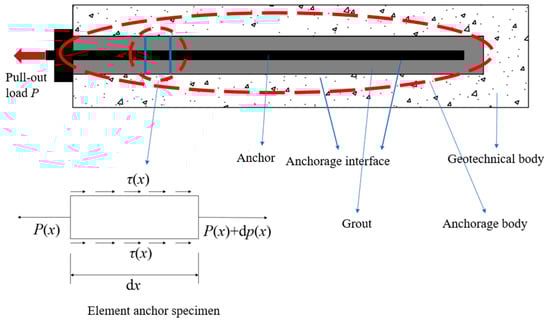
Figure 1.
Schematic of interface characterization using element anchor specimens.
To ascertain the genuine stress state of the anchor, numerous scholars have conducted extensive research on the load transfer mechanism within the anchorage section. Phillips discovered an exponential distribution of shear stress along the anchor based on measured data [8]. Benmokrane et al. compared the impact of different grouting materials and anchoring lengths on bolt performance, providing an empirical equation for pull-out resistance and a straightforward bond-slip constitutive model [9]. Cai et al. introduced an analytical model for predicting the axial force of grouting bolts, elucidating the interaction mechanism between bolts and soft rock masses. They identified a position of maximum anchoring length, beyond which the axial force ceases to increase [10]. Richard et al. and Rong et al. established a hyperbolic model for load transfer in the anchorage section, deriving the functional expression [11,12]. These studies collectively reveal that shear stress at the anchorage interface is non-uniform and does not follow a linear distribution. However, peak shear stresses from these models are typically highest at the pulling end, gradually decreasing along the depth of the anchorage. These methods overlook the gradual onset of plastic deformation or debonding as pull-out stress increases. Subsequently, Ren F.F. established a tri-linear bond-slip model of shear stress and shear displacement based on the stress softening of the anchorage body. He found that the peak shear stress does not necessarily occur at the pulling end [13]. Changfu Chen et al., Minghua Huang et al., and Lin Zhang et al. employed exponential function models, double exponential function models, and exponential–hyperbolic composite models, respectively [14,15,16]. They aimed to depict the relationship between shear stress and shear displacement, simulating the entire load transfer process at the anchorage interface. Results indicated that the peak shear stress initially appeared at the pulling end when the pull-out load was small. With increasing tensioning load, yielding phenomena manifested at the pulling end, causing the shear stress peak to shift towards the depth of the anchorage section. Zhang et al. categorized the anchor pull-out process into three stages: elastic, plastic, and residual. Hence, residual shear stress emerges as a significant factor influencing the load transfer behavior of the anchor interface [17].
In summary, existing load transfer models for the anchorage section each have their limitations. The tri-linear bond-slip model effectively captures the different stages of anchor behavior with increasing pullout force, but falls short in reflecting the nonlinear characteristics of shear stress and shear displacement [18,19,20,21,22]. On the other hand, the hyperbolic model accurately represents the nonlinearities of shear stress and shear displacement but neglects the softening of the anchorage body [11,12,23]. Meanwhile, the double exponential curve model provides a comprehensive response to various stages in the anchor pullout process, but its complexity and lack of an easily derived analytical solution hinder its practical applications in engineering [15,16,24]. To address these shortcomings, this paper proposes a novel model based on the elasto-plastic relationship. The model combines linear and nonlinear components to describe shear stress and displacement at the anchorage interface. By deriving the distribution of axial and shear stresses at different stages of anchor pullout using the anchor’s load transfer equation, the paper aims to offer insights into the patterns of load transfer and the characteristics of the anchor pullout process as the pullout load increases.
2. Basic Equations for Anchor Load Transfer
The steps involved in deducing the anchorage mechanism through mathematical formulas are as follows: Firstly, acquire the basic equations of load transfer by analyzing the stress balance of the microelement body. Next, solve the basic equations of load transfer using the bond slip model of the anchorage body. Finally, draw conclusions on the function expressions describing the distribution of axial force and shear stress.
A microelement body with a length of dx is chosen as the subject of study in the anchored section of the anchor bar, as illustrated in Figure 1. Due to the small size of the microelement body, it is reasonable to approximate that the shear stress distribution on this microelement is uniform.
According to the axial force, equilibrium can be obtained:
where p(x) is the axial load of the anchorage body, τ(s(x)) is the shear stress of the anchorage interface, and U is the perimeter of the anchorage body.
And the micrometric body satisfies
where ε(x) is the axial strain of the anchorage body, and E and A are the Young’s modulus of elasticity and cross-sectional area of the anchorage body.
The basic equations of load transfer can be obtained by substituting Equation (1) into Equation (3),
where s(x) is the shear displacement of the anchorage interface, and the value of the shear displacement s(x) is equal to the value of the axial displacement u(x), under the action of the axial load.
3. Analytical Solution for Anchor Load Transfer
The key to solving the load transfer problem in the anchored segment of the anchor lies in τ(s(x)), the expression for the shear-slip model derived from basic Equation (4). In this study, a segmented function is employed to depict the bond-slip characteristics at the interface between the anchorage body and the surrounding geotechnical body under tensioning, as depicted in Figure 2. During low pull-out loads, the interface is in the elastic stage (OA segment in the figure), where the shear stress and shear displacement exhibit a linear growth relationship. As the pull-out load increases and surpasses the limit value τ1, the interface softens, entering the plastic stage (AB section in the figure). Here, a small increase in the pull-out load results in significant plastic deformation, leading to a nonlinear relationship between interface shear stress and shear displacement. A continued increase in the pull-out load causes the shear displacement to exceed the plastic limit displacement S2. This results in a loose slip phenomenon between the anchorage body and the surrounding geotechnical body, initiating the debonding stage (BC section in the figure). The interaction stages between the anchorage body and the geotechnical body are illustrated in Figure 3. Consequently, the mathematical expression for the shear-slip constitutive model at the interface between the anchorage body and the surrounding geotechnical body is
where τ is the interface shear stress, s is the interface shear displacement, τ2 is the residual shear strength of the anchorage section, K is the shear stiffness coefficient when the anchorage section and the surrounding geotechnical body are in an elastic state, and S1 and S2 are the limit value of the shear strength of the anchorage section and the shear displacement corresponding to the residual strength, respectively.
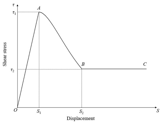
Figure 2.
Linear–nonlinear bond-slip model.
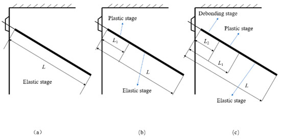
Figure 3.
Stages of interaction between anchorage body and rock mass: (a) elastic state; (b) plastic state; (c) debonding state.
3.1. Elastic State Solutions
Bringing Equation (5) into Equation (4) yields the elastic stage differential equation:
The generalized solution of the differential Equation (6) is
where C1 and C2 are coefficients to be determined, and . Substituting Equation (7) into Equations (3) and (5) yields the distribution of axial and interfacial shear stresses, respectively, in the anchorage body in the elastic phase:
For the elastic deformation stage, the boundary conditions of the problem are , , where L is the length of the anchoring section, from which the coefficients C1 and C2 corresponding to the elastic phase can be obtained as follows:
Further, the expressions for the anchorage body’s displacement, axial force, and interfacial shear stress in the elastic phase can be obtained as follows:
When , for the pulling end shear stress, the part of the anchor near the pulling end will enter the plastic stage, from which the elastic ultimate load of the anchor can be obtained as follows:
From Equation (14), it can be seen that when 2αL = 6, , the limiting length of the elastic stage can be obtained as Lt = 3/α; it is also difficult to increase the elastic ultimate load, when the length of the anchoring section exceeds this value, which can be simplified as Equation (15).
3.2. Plastic State Solution
When the pullout load surpasses the elastic limit load (Ptk), the anchorage body transitions into a state that is partially elastic and partially plastic. In this state, the expressions for displacement, axial force, and shear stress of the anchorage body should be segmented. The elastic part can follow Equations (7)–(9) seamlessly, while the subsequent section deals with the plastic part of the solution expressions. Reference [25] indicates that the shapes of the distribution curves of axial force and shear stress in the anchorage body are influenced by the magnitude of the applied load, whereas the shapes of the distribution curves of shear displacement remain stable. Therefore, based on the measured data of the anchorage body shear displacement in the case study by Bo Liu et al. [26], the expression for the shear displacement distribution curve is obtained through fitting. The fitting results, shown in Figure 4, demonstrate an ideal fit. The expression for anchorage body shear displacement is as follows:
where a, b, and c are coefficients to be determined.
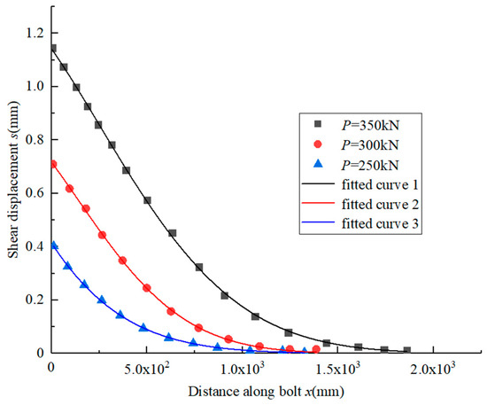
Figure 4.
Displacement curves of anchorage body.
Bringing Equation (16) into Equations (2) and (3) yields expressions for the distribution of axial and shear stresses in the plastic part of the anchorage body:
From Figure 3b, the boundary conditions for the plastic stage are , , , , and , where L1 is the length of the plastic part. The coefficients to be determined for the elastic part C1, C2 and the coefficients to be determined for the plastic part a, b, c can be solved as follows:
As the pullout load increases, the anchor will reach the plastic limit state when the displacement at the top of the anchored section reaches S2, which is ; simultaneously, the value of the coefficient to be determined a can be solved, and at this time the pull-out load is called the plastic limit load Psk. Bring the coefficient of determination a into Equation (19) to solve for the value of L1, which is the limiting length of the plastic part in the plastic limit state Ls, and bring Ls into to solve the plastic limit load Psk.
3.3. Debonding State Solution
As the pull-out load surpasses the plastic limit load (Psk), the pulling end of the anchored section initiates the debonding stage. In this phase, the plastic and elastic components persist in the deeper regions. As illustrated in Figure 2, near the pulling end of the anchored section, the interfacial shear stress in the debonding part is represented by the residual stress (τ2). The elastic and plastic elements in the deeper section can further adhere to Equations (7)–(9) and Equations (16)–(18). Subsequently, the expression for the debonding part can be derived through the following solving process.
Bringing Equation (5) into Equation (4) gives the differential equation for the debonding part as
The generalized solution of the differential Equation (20) is
where C3 and C4 are coefficients to be determined, and . Bringing Equation (21) into Equation (3) yields the axial force distribution in the debonding part of the anchoring section as
From Figure 3c, the boundary condition for the slip stage is , , where L2 is the length of the debonding section. The coefficients to be determined for the corresponding slip sections C3, C4 can be solved as follows:
From the continuity condition of displacement and axial force at any cross-section of the anchor, we can see that . Bringing in Equation (23) gives
Using Equation (24), the length (Lh) of the debonding section under any pullout load (P) in the debonding stage can be computed, specifically as Lh = L2. Similarly, knowing the maximum allowable length (Lh) of the debonding part allows the back-calculation of the maximum ultimate load capacity of the anchor, denoted as Pumax = P. The calculation method for the entire process of the anchoring system under the pull-out load at each stage is illustrated in Figure 5.
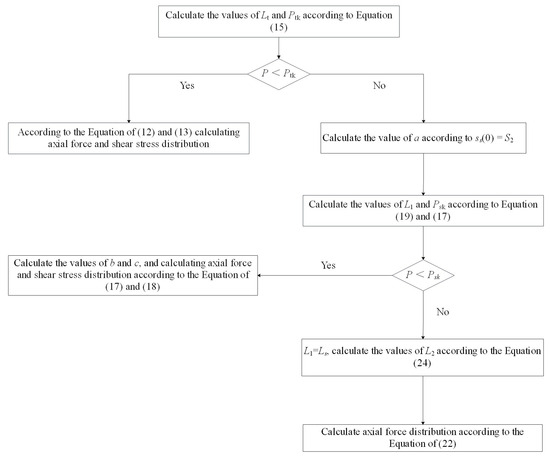
Figure 5.
The flow chart of the calculation method of the anchoring system at each stage.
4. Example Verification and Engineering Application
4.1. Example Verification and Analysis
In a field pullout experiment conducted by Bo Liu et al. [26] in a mountainous area, as depicted in Figure 6, the anchoring bar had a diameter (D) of 42 mm, a Young’s modulus (E) of 210 GPa, and an anchoring length (L) of 3 m. The grouting body was composed of fine gravel concrete with a uniaxial compressive strength of 27.10 MPa and a deformation modulus of 26 GPa. The diameter of the drilled holes was 150 mm. Strain gauges were strategically placed at 150 mm intervals along the anchored section, capturing changes in displacement and axial force at the top of the anchor during the upward pull-out process. The interfacial mechanical parameters obtained were as follows: S1 = 0.21 mm, S2 = 0.38 mm, τ1 = 3.84 MPa, τ2 = 1.15 MPa.
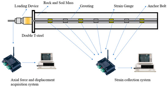
Figure 6.
Diagrammatic drawing of anchor pull-out tests.
Using Equations (14) and (15), the ultimate length of the elastic state of the anchor (Lt) is determined to be 1.045 m, with an ultimate elastic load (Ptk) of 175 kN. Building on the research outlined in Section 3.2, the ultimate length of the plastic state (Ls) is calculated as 207 mm, and the ultimate plastic load (Psk) is found to be 271 kN. Incorporating field-measured data into Equations (11), (12), (16), (17), (21), and (24), the theoretical curve depicting the relationship between pull-out load and anchor displacement is obtained, as illustrated in Figure 7. The figure reveals distinct stages as the pull-out load increases, namely the elastic stage (OA), plastic stage (AB), and debonding stage (BC). The OA stage represents the elastic phase, with point A acting as the boundary between the elastic and plastic stages. Section AB signifies the plastic stage, with point B marking the transition to the plastic-debonding stage. Section BC corresponds to the debonding stage. Observing Figure 7, the load–displacement relationship obtained through the theoretical calculation aligns well with the measured data. The variance between the measured and calculated values falls within the range of 1.3% to 8.8%, affirming the validity of the theoretical derivation.
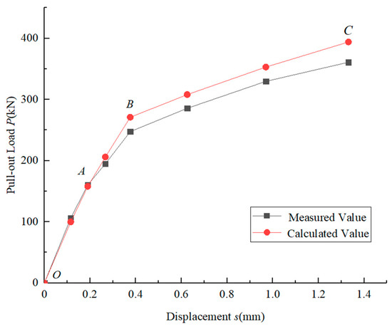
Figure 7.
Load–axial displacement curves of the anchor.
In Figure 8, a comparison of the pull-out load–displacement prediction curve generated by the model presented in this paper is shown alongside other published mathematical models, including the trilinear bond-slip model, double exponential function model, and exponential–hyperbolic composite model. The results of the comparison indicate that, during the elastic state of the anchorage body, the calculation outcomes of each model are relatively close. However, as the anchorage body transitions into the plastic and debonding states, differences emerge in the calculated results and the curve trends. This discrepancy may arise from varying assumptions each model makes for the plastic stage, resulting in a more significant difference in debonding state results compared to the elastic state. It is worth noting that the length of the plastic state of the anchorage body in this project is relatively short, which could contribute to a less pronounced difference in the results during the plastic state.
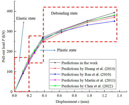
Figure 8.
Comparison of the predictions of pull-out load–displacement responses between the published mathematical models [13,14,15,18] and the model in this work.
Utilizing Equations (12), (17), and (22), and field-measured results, the axial force distribution curves of the anchor along the anchoring depth under pull-out loads of P = 160 kN, 250 kN, and 300 kN are calculated, as depicted in Figure 9. Notably, the calculated theoretical curve of axial force distribution aligns well with the measured curve, effectively reflecting the axial force distribution in the anchoring section of the anchor under the influence of pulling forces. In Figure 9, as the pull-out load increases, the axial force of the anchor does not distribute evenly and exhibits a nonlinear pattern. It gradually transmits towards the far end of the anchoring section, highlighting the following specific characteristics:
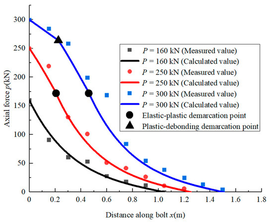
Figure 9.
Axial force along the anchorage segments.
- (1)
- At a pull-out load of P = 160 kN, which is below the elastic limit load (Ptk), the interface around the anchoring section is in an elastic state. Consequently, the axial force gradually decreases to 0 towards the far end. There is no axial force distribution beyond the anchoring depth of 1.045 m, representing the limit length (Lt) of the elastic state. The axial force curve exhibits a concave form under these conditions.
- (2)
- As the pull-out load increases, reaching P = Ptk, the shear stress at the top of the anchoring section hits the ultimate shear strength τ1. At this juncture, the anchoring section begins to soften, and the portion near the top of the anchoring section enters the plastic state. When the pull-out load reaches P = 250 kN, a section of the anchor undergoes plastic softening. This specific segment, known as the plastic part, is characterized by a length (L1) equal to 0.168 m, forming a slightly convex curve on the axial force distribution curve. This curvature arises because the shear stress in the plastic softening part is less than the ultimate shear strength τ1, resulting in a reduced transmission rate of axial force to the distant part of the anchoring section. The segment with an anchorage length greater than 0.168 m remains in the elastic state, and the axial force is transmitted to an anchorage depth of 1.213 m.
- (3)
- As the pull-out load continues to rise, reaching P = Psk, the shear stress at the top of the anchoring section decreases to the residual shear strength τ2. At this critical point, the anchoring section is on the brink of cracking and sliding, and the region near the top of the anchoring section enters a debonding state. At a pull-out load of P = 300 kN, the length of the anchor undergoes debonding, with the length of the debonding part (L2) measuring 0.225 m. This debonding part is represented as a straight line on the axial force curve since the shear stress in the slipping section remains constant. Within the segment with an anchoring length between 0.225 m and 0.432 m, the material still remains in a plastic state, and the length of the plastic part (L1) is 0.207 m. The portion with an anchoring length greater than 0.432 m remains elastic, and the axial force is transmitted to an anchoring depth of 1.477 m.
4.2. Engineering Application
The residential foundation pit project at 2017NJY-11 block in Dongyong Town, Guangzhou, China, employs prestressed anchor cables to support the foundation pit wall. The anchor holes, with a diameter of 150 mm, are designed to accommodate 5 × 7Φ5 steel strand anchor cables featuring a Young’s modulus of 195 GPa. An anchorage acceptance test for the anchor cables was conducted to assess their performance under the design load, serving as a basis for project acceptance. The experiment primarily comprised an experimental loading device, a force and displacement measuring device, and a data acquisition and processing system. The loading device utilizes a pressure plate reaction device, with the pull-out load provided by a QFZ1000-20 model hydraulic jack. The force and displacement measuring device includes a pressure gauge of model L26091517 and a displacement sensor of model BL100-V-1000. The data acquisition and processing system displays the pull-out load and displacement data of the pulling end of the anchor on the computer.
The sections of the A, B, and C anchor cables embedded in the ground had lengths of 42 m, 40 m, and 42 m, respectively. The anchor cable passed through the ground from top to bottom, traversing through silt, a layer of loose and slightly dense silt, and strongly weathered argillous sandstone. The experiment was conducted in accordance with the Technical Specification for Ground Anchors (CECS22:2005) [27], utilizing graded loading and unloading. The maximum experimental load applied was 1.2 times the design value of the anchor. The cyclic loading experiments followed the sequence outlined in Table 1. Displacements under the load were recorded over ten cycles, and the next level of load was applied when the difference between ten consecutive measurements did not exceed 0.01 mm. The maximum experimental loads were 780 kN, 660 kN, and 720 kN, respectively. Table 2 and Figure 9 depict the outcomes of the experiments, illustrating the pull-out load and displacement at the anchor head.

Table 1.
Load grade and duration of acceptance test of anchors.
Table 2.
Pull-out test data.
Taking cable A as an example for engineering application calculation, Figure 10 reveals significant changes in the slope of the load–displacement curve when the pull-out load (P) is at 234 kN and 546 kN. Accordingly:
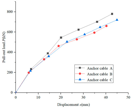
Figure 10.
Load–axial displacement curves of the anchor cable.
When P < 234 kN, the anchoring section of the anchor is in the elastic stage.
For 234 kN ≤ P < 546 kN, the anchoring section enters the plastic stage.
When P ≥ 546 kN, the anchoring section enters the debonding stage. Here, the elastic limit load (Ptk) is 234 kN, and the plastic limit load (Psk) is 546 kN.
By substituting Ptk = 234 kN, Psk = 546 kN, S1 = 6.79 mm, and S2 = 20.07 mm into Equations (12)–(14), (17)–(19), (22), and (23), the mechanical parameters of the anchorage interface are obtained: τ1 = 191 kPa, τ2 = 44.5 kPa. Further, bringing the limit length of the debonding part (Lh) = 37.68 m into Equation (24) yields Pumax = 1065.8 kN. Considering the design load (P) for the axial pull of the anchor in this project as 650 kN, the safety factor (Fs = Pumax/P) for anchor cable A is calculated as 1.64. This meets the specified anchorage safety factor requirement of 1.6 according to the specification [27]. The calculation method for cables B and C mirrors that of cable A and will not be reiterated here. The results for all three cables are summarized in Table 3.
Table 3.
Interface parameters of each anchor cable and calculation results.
5. Conclusions
Through the establishment of a composite model incorporating linear and nonlinear shear displacement at the anchorage interface in distinct stages, analytical solutions for the axial force, shear stress, displacement, and maximum bearing capacity of the anchor at each stage have been derived. These solutions have been validated against field-measured data. Concurrently, an analysis of the load transfer mechanism throughout the entire process of the anchor under varying pull-out loads has been conducted. The primary conclusions drawn from this analysis are as follows:
- (1)
- The step-wise linear-nonlinear bond-slip composite model is presented in the form of a single-peak curve. As the pull-out load increases, the anchor surface sequentially transitions through the elastic stage, the plastic stage, and the debonding stage. The model adeptly captures the elastic characteristics of the elastic stage, the softening and nonlinear attributes of the plastic stage, and the residual characteristics of the debonding stage.
- (2)
- In the pulling process, when the pull-out load is small, the anchorage interface remains in an elastic state, and the maximum shear stress is situated at the pulling end of the anchor. Consequently, the axial force experiences a rapid decline along the anchoring depth. As the pull-out load surpasses the elastic limit load, the plastic state initiates from the pulling end of the anchor, and the maximum shear stress is located at the boundary point between the elastic and plastic states. Upon exceeding the plastic limit load, the debonding state begins from the pulling end of the anchor, leading to the continued development of axial force into deeper sections. Furthermore, it is noteworthy that most measured values of axial force are less than the calculated values, indicating that the prediction method in this paper tends to be on the side of safety.
- (3)
- The load–displacement curves and axial loading distribution of the anchor were determined using the load transfer method based on the step-wise linear-nonlinear bond-slip composite model. The theoretical values were extensively validated against fieldwork published in the literature. The calculation method was applied to an actual project, revealing the shear responses of the anchor during the pull-out test. The output safety factor met the requirements of relevant specifications, affirming the reliability and practicality of the method.
Author Contributions
This paper was accomplished based on collaborative work by the authors. Conceptualization, Z.C.; Funding acquisition, Y.W.; Data curation, K.Z. and D.W.; Investigation, D.W.; Project administration, Y.W. and D.W.; Formula derivation, Z.C.; Validation, Z.C. and D.W.; Writing—original draft, Z.C.; Writing—review and editing, Y.W. and K.Z. All authors have read and agreed to the published version of the manuscript.
Funding
This study was supported by the Guangdong Province science and technology innovation plan project (2021ZHJKJ-13). We are grateful for the support of the science and technology innovation plan project.
Institutional Review Board Statement
Not applicable.
Informed Consent Statement
Not applicable.
Data Availability Statement
The data presented in this study are available on request from the corresponding author. The data are not publicly available because they came from a project report.
Conflicts of Interest
Daidong Wei was employed by Guangzhou Chemical Grouting Engineering Co., Ltd., CAS. The remaining authors declare that the research was conducted in the absence of any commercial or financial relationships that could be construed as a potential conflict of interest.
References
- Guo, F.X.; Tu, M.; Dang, J.X. Analysis and Design of Protection Device for Anchor Cable Pull-Out in High-Stress Roadways. Appl. Sci. 2023, 13, 12023. [Google Scholar] [CrossRef]
- Liu, Y.G.; Xia, K.; Wang, B.T.; Le, J.; Ma, Y.Q.; Zhang, M.L. Experimental Investigation on the Anchorage Performance of a Tension–Compression-Dispersed Composite Anti-Floating Anchor. Appl. Sci. 2023, 13, 12016. [Google Scholar] [CrossRef]
- Li, J.; Chen, S.X.; Yu, F.; Jiang, L.F. Reinforcement Mechanism and Optimisation of Reinforcement Approach of a High and Steep Slope Using Prestressed Anchor Cables. Appl. Sci. 2020, 10, 266. [Google Scholar] [CrossRef]
- Zou, J.F.; Zhang, P.H. Analytical model of fully grouted bolts in pull-out tests and in situ rock masses. Int. J. Rock Mech. Min. Sci. 2019, 113, 278–294. [Google Scholar]
- Tang, Y.F.; Jiang, D.H.; Wang, T.X.; Luan, H.J.; Liu, J.W.; Zhang, S.H. Research on the Mechanism of the Passive Reinforcement of Structural Surface Shear Strength by Bolts under Structural Surface Dislocation. Appl. Sci. 2023, 13, 543. [Google Scholar] [CrossRef]
- Yang, D.; Wang, Q.C.; Jiang, Z.Q.; Yang, D.X. A Multi-Segment Expanded Anchor for Landslide Emergency Management. Appl. Sci. 2022, 12, 12985. [Google Scholar] [CrossRef]
- Chen, J.; Li, D. Numerical simulation of fully encapsulated rock bolts with a tri-linear constitutive relation. Tunn. Undergr. Space Technol. 2022, 120, 104265. [Google Scholar] [CrossRef]
- Phillips, S.H.E. Factors Affecting the Design of Anchorages in Rock; Cementation Research Ltd.: London, UK, 1970. [Google Scholar]
- Benmokrane, B.; Chennouf, A.; Mitri, H.S. Laboratory evaluation of cement-based grouts and grouted rock anchors. Int. J. Rock Mech. Min. Sci. 1995, 32, 633–642. [Google Scholar] [CrossRef]
- Cai, Y.; Esaki, T.; Jiang, Y.J. An analytical model to predict axial load in grouted rock bolt for soft rock tunnelling. Tunn. Undergr. Space Technol. 2004, 19, 607–618. [Google Scholar] [CrossRef]
- Richard, R.M.; Abbott, B.J. Versatile elastic-plastic stressstrain formula. J. Eng. Mech. Div. 1975, 101, 511–515. [Google Scholar] [CrossRef]
- Wong, K.S.; Teh, C.I. Negative skin friction on piles in layered deposits. J. Geotech. Eng. 1995, 121, 457–465. [Google Scholar] [CrossRef]
- Ren, F.F.; Yang, Z.J.; Chen, J.F.; Chen, W.W. An analytical analysis of the full-range behaviour of grouted rockbolts based on a tri-linear bond-slip model. Constr. Build. Mater. 2010, 24, 361–370. [Google Scholar] [CrossRef]
- Chen, C.F.; Zhu, S.M.; Zhang, G.B.; Morsy, A.M.; Zornberg, J.G.; Mao, F.S. A Generalized Load-Transfer Modeling Framework for Tensioned Anchors Integrating Adhesion–Friction-Based Interface Model. Int. J. Geomech. 2022, 22, 04022036. [Google Scholar] [CrossRef]
- Huang, M.H. Analysis on Pullout Load Transfer Mechanism of Geotechnical Anchor and Its Validating Monitor with Smart FRP Anchor. Ph.D. Thesis, Harbin Institute of Technology, Harbin, China, 2014. [Google Scholar]
- Zhang, L.; Wang, M.; Zhao, H.B.; Chang, X. Uncertainty quantification for the mechanical behavior of fully grouted rockbolts subjected to pull-out tests. Comput. Geotech. 2022, 145, 104665. [Google Scholar] [CrossRef]
- Zhang, W.L.; Huang, L.; Juang, C.H. An analytical model for estimating the force and displacement of fully grouted rock bolts. Comput. Geotech. 2020, 117, 103222. [Google Scholar] [CrossRef]
- Martin, L.B.; Tijani, M.; Hadj-Hassen, F. A new analytical solution to the mechanical behaviour of fully grouted rockbolts subjected to pull-out tests. Constr. Build. Mater. 2011, 25, 749–755. [Google Scholar] [CrossRef]
- Xiao, S.J.; Chen, C.F. Mechanical mechanism analysis of tension type anchor based on shear displacement method. J. Cent. South Univ. Technol. 2008, 15, 106–111. [Google Scholar] [CrossRef]
- Ma, S.Q.; Zhao, Z.Y.; Nie, W.; Gui, Y.L. A numerical model of fully grouted bolts considering the tri-linear shear bond–slip model. Tunn. Undergr. Space Technol. 2016, 54, 73–80. [Google Scholar] [CrossRef]
- Nemcik, J.; Ma, S.Q.; Aziz, N.; Ren, T.; Geng, X.Y. Numerical modelling of failure propagation in fully grouted rock bolts subjected to tensile load. Int. J. Rock Mech. Min. Sci. 2014, 71, 293–300. [Google Scholar] [CrossRef]
- Xu, C.; Li, Z.H.; Wang, S.Y.; Wang, S.R.; Fu, L.; Tang, C.N. Pullout Performances of Grouted Rockbolt Systems with Bond Defects. Rock Mech. Rock Eng. 2018, 51, 861–871. [Google Scholar] [CrossRef]
- Zhao, M.H.; Huang, Y.J.; Huang, M.H. Study on nonlinear calculation method of load transferring along tensile anchor rod base on finite difference method. J. Railw. Sci. Eng. 2018, 15, 1963–1970. [Google Scholar]
- Zhou, S.C.; Zhu, W.C.; Yu, S.S. Analysis of load transfer mechanism for fully grouted rockbolts based on the bi-exponential shear-slip model. Chin. J. Rock Mech. Eng. 2018, 37, 3817–3825. [Google Scholar]
- Zhou, B.S.; Wang, B.T.; Liang, C.Y.; Wang, Y.H. Study on load transfer characteristics of wholly grouted bolt. Chin. J. Rock Mech. Eng. 2017, 36, 3774–3780. [Google Scholar]
- Liu, B.; Huang, L.; Li, D.Y. Analytical Formulation on the Mechanical Behavior of Anchorage Interface for Full-Length Bonded Bolt. Appl. Mech. Mater. 2012, 166–169, 3254–3257. [Google Scholar] [CrossRef]
- CECS22:2005; Technical Specification for Ground Anchors. China Planning Press: Beijing, China, 2005.
Disclaimer/Publisher’s Note: The statements, opinions and data contained in all publications are solely those of the individual author(s) and contributor(s) and not of MDPI and/or the editor(s). MDPI and/or the editor(s) disclaim responsibility for any injury to people or property resulting from any ideas, methods, instructions or products referred to in the content. |
© 2024 by the authors. Licensee MDPI, Basel, Switzerland. This article is an open access article distributed under the terms and conditions of the Creative Commons Attribution (CC BY) license (https://creativecommons.org/licenses/by/4.0/).