Comparative Analysis of Nucleus Segmentation Techniques for Enhanced DNA Quantification in Propidium Iodide-Stained Samples

Abstract

Digitization in pathology and cytology labs is now widespread, a significant shift from a decade ago when few doctors used image processing tools. Despite unchanged scanning times due to excitation in fluorescent imaging, advancements in computing power and software have enabled more complex algorithms, yielding better-quality results. This study evaluates three nucleus segmentation algorithms for ploidy analysis using propidium iodide-stained digital WSI slides. Our goal was to improve segmentation accuracy to more closely match DNA histograms obtained via flow cytometry, with the ultimate aim of enhancing the calibration method we proposed in a previous study, which seeks to align image cytometry results with those from flow cytometry. We assessed these algorithms based on raw segmentation performance and DNA histogram similarity, using confusion-matrix-based metrics. Results indicate that modern algorithms perform better, with F1 scores exceeding 0.845, compared to our earlier solution’s 0.807, and produce DNA histograms that more closely resemble those from the reference FCM method.

1. Introduction

DNA ploidy analysis is a laboratory technique that assesses the DNA content in a cell’s nucleus, helping classify cells based on their ploidy status. This indicates the number of complete chromosome sets in a cell. Ploidy analysis is particularly important in cancer research for identifying abnormal DNA content, supporting diagnosis and treatment decisions.

To measure DNA content, the sample must be stained with a dye that stays in the sample in amounts proportional to the DNA content of the sample at the given location. There are multiple staining options; the samples of this study were propidium iodide-stained. This type of sample can be digitized using fluorescent imaging. The dye, after being excited with a light of specific wavelength, emits light of a different wavelength that can be measured.

The sample can be cell nuclei, extracted from any body tissue that contains DNA. These analyses are usually done on a flow cytometer (FCM), an appliance that processes the sample in a liquid form, examining the objects passing in a single row in a capillary tube between usually a laser source and a detector [1]. This technology is prevalent today, and developments are added to the original concept, both on the appliance and the reagent side [2]. Our project explores an alternative approach to achieve the same goal, via digital imaging. The light emitted by the fluorochrome is captured by a digital camera, creating input data for image processing technologies. This technique is called image cytometry (ICM). It takes merit from the digitalization of pathology and cytology labs being equipped with machines to digitize glass slide specimens, especially those capable of fluorescent operation. In the beginning, research-oriented users adopted the benefits of digital samples. Then brightfield, immunohistochemistry (IHC) samples were evaluated more and more frequently [3,4,5]. Today, diagnostic laboratories are progressively adopting digital pathology [6,7], with a continually expanding range of applications [8,9,10]. Recently, deep learning-based methods are explored not only for object segmentation but for quality control, denoising or as an upscaling technology [6,7,8].

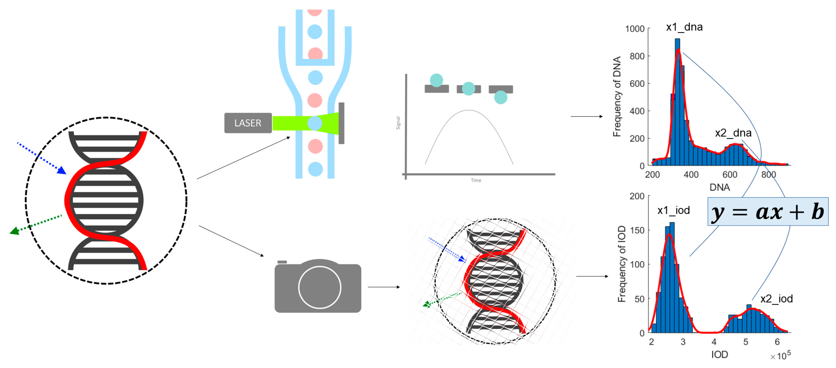
This project is to create an approach based on image processing that produces the DNA content measurements needed for ploidy analysis; from nuclei segmentation through feature extraction, to comparison of results to FCM ones derived from the same samples, calibration (Figure 1) and finally ploidy analysis.

The evaluation of these samples can be done via computer-based image processing means. This choice holds possible benefits: lab desk space, a fixed cost, can be reduced by consolidating tools, thereby reducing maintenance expenses. Small diagnostic labs considering digital pathology or handling a higher imaging workload, may opt for the ICM approach as a replacement for FCM. For those adopting ICM, the introduction of ploidy analysis is streamlined, requiring only the extension of the sample preparation process to include placement on a glass slide and coverslipping. For labs with a heavier imaging workload, a glass-slide-only workflow becomes feasible. Additionally, the benefit of extended specimen storage, whether as a glass slide or in this case as a digital image, is crucial for future research projects, case consultation or teaching.

Measuring the overall accuracy of an image analysis algorithm can be defined on multiple levels, and through multiple metrics. In this study we applied two approaches: one is to measure the segmentation algorithms’ raw accuracy compared to the ground truth; the other is to measure the population-level DNA content’s similarity to the FCM method.

In our previous work, we proposed a calibration method to align image cytometry (ICM) results with those of flow cytometry (FCM) for DNA ploidy analysis, using healthy samples with known properties as references. The calibration approach involves analyzing the DNA content histograms from both methods, with the goal of developing a transfer function that ensures ICM can replicate the accuracy of FCM. Specifically, healthy samples containing at least two object populations—one with theoretically double the DNA content of the other—serve as a reference point, with these populations represented by their mean values on the DNA histogram’s x-axis. Ploidy analysis examines these peaks, and their relation allows for an evaluation of the accuracy of our technique. In the current study, we extend this work by focusing on optimizing nucleus segmentation, a key step in enhancing the accuracy of ICM histograms, thereby further improving the calibration process and ensuring better alignment with FCM.

The image analysis pipeline is usually comprised of a segmentation step to localize the nuclei on the sample. A separation step of some kind is necessary. The sample being a solution, the nuclei tend to form groups or clumps. Those are frequently segmented as one single object, thus greatly influencing the detection quality. After that, features are measured, like integrated optical density which represents the amount of DNA content of an object. These features then can be used to classify the nuclei, and consequently conclude the ploidy analysis: classify the cell population to be normal, or whether some deviation can be detected. Comparison of FCM and our proposed ICM method was published in [9]. This article focuses on the object detection/segmentation part of the process, highlighted in Figure 2.

The quality of such an algorithm is usually measured via comparison to a reference or ground truth. This type of information is hard and costly to obtain, though public datasets for similar purposes can be found [10]. The ground truth dataset was created to establish a means of measurement for the counting problem, to be able to count the matching pairs of annotation and detected object along with all the other remaining cases.

The resulting ground truth is a set of coordinate pairs that mark the location of each object (nucleus) visible on the digital sample. In this article we aim to evaluate the algorithms examined regarding their object detection capability. Our priority goal was to evaluate object localization, but not extent.

We propose that by increasing object segmentation performance, the similarity between the FCM and ICM results will also measurably increase.

Digital pathology tools, able to create and store single-point annotations, have been on the field for a long time. It is safe to assume that there are many projects where such annotations were used to designate objects of interest. Generating a reference dataset is one of the main expenses in an image analysis (object detection, segmentation) project. It seems logical to explore the possibility of re-using them, in some cases, when creating the annotation from scratch is a costly solution, or data are scarce, similarly to this project.

Based on the pair of reference and measurement results, each object can be classified into four classes: true positive (TP), true negative (TN), false positive (FP) and false negative (FN). This information is collected into a confusion matrix, and algorithm quality measures are calculated from that. This gives the framework of comparison for the algorithms examined.

Image processing on fluorescent samples is quite different from analyzing brightfield samples. Fluorescent samples are generated in smaller quantities, caused by the cost of the technique itself. Digitization time is heavily dependent on the appliance and is mostly governed by the excitation time. Glass slide samples can take more than an hour, or even multiple hours to digitize. The data to measure are usually separated into single image channels, which simplifies the image processing task. In the case of this project, low exposure times and single channel demand resulted in a 5–10-min long digitization process. Sample thickness and light scatter in the sample makes the object boundaries harder to discern. Generally, the task of detecting/segmenting objects on fluorescent samples can be a less complex problem, that enables the usage of algorithms of simpler construction. This is fortunate, because more complex supervised deep learning AI models need considerably more annotated training data, and usually unsupervised methods need even more data. Achieving improvements in that direction seems to be an endeavor gradually more and more complicated. Transfer learning might be an option to consider, using available models and using and extending their training set with task-specific samples.

In diagnostics, AI image analysis is less widespread/accepted now, but this is changing rapidly. Explainability and tractability are among the causes (through regulatory aspects). There are projects investigating better explainable segmentation algorithms [11], that try to deal with these aspects of modern AI. The algorithms we selected have the advantage of still being simple in concept and solving only the segmentation part of the problem, thus the risks involved remain controllable, while maintaining the equilibrium of cost and performance.

2. Materials and Methods

2.1. Samples

For this evaluation we used 15 samples of leftover healthy human blood samples containing only propidium iodide-stained cell nuclei. We placed samples on a glass slide after serving their original purpose in a flow cytometer. We coverslipped and digitized them using a glass slide scanner produced by 3DHISTECH Ltd., Budapest, Hungary (Pannoramic Scan, fluorescent setup, 5 MP sCMOS camera, 40× (Carl Zeiss AG, Jena, Germany) objective lens and an LED-based light source). The resulting resolution of the images was 0.1625 µm/pixel (compressed with jpeg, to quality 80). The ICM measurements were taken on sub-samples of these samples, sampled as lab protocols demand, in the amount to fit on a glass-covered glass slide. We identified the samples by their sequential indices throughout the assay (1M01–1M20). The samples could contain a droplet of sample of the size of approximately 15 mm in diameter. This meant an approximately 180 mm² area populated with nuclei, roughly 7 gigapixels to process. The algorithms’ input was an 8-bit, single channel image, that was ingested by the algorithms in a tiled manner.

The FCM measurements were conducted using a Becton Dickinson FACSCAN flow cytometer with the CellQuest software (version 3.1, both hardware and software by Becton Dickinson, Franklin Lakes, NJ, USA). The samples were stained with PI for visualization of DNA content and contained more than 10,000 measured nuclei each.

2.2. Annotation

Annotation of medical images is a complex topic [12]; the task at hand is complex because of the simplicity of the available annotation data.

For the development of Algorithm 1 more than 20,000 objects were annotated with single-point markers. This is usually called landmark annotation. We used these data to evaluate and compare the selected algorithms.

To reduce the annotation workload, we selected 1 mm² rectangular regions on the sample for validation, containing from ~830 to ~2200 annotated nuclei. We worked with an expert with laboratory experience in placing the annotations. Cells visible on the digital samples were annotated using the Pannoramic Viewer (1.15.4) software’s Marker Counter tool. For this purpose, we selected regions without visible artefacts (bubbles, clumping, unwashed/overexposed staining). The annotation process took 20–40 min per slide, based on nucleus content.

Multiple approaches can be taken when using these types of annotation data for the evaluation, but the template is simple, as summarized in Figure 3.

2.3. Environment

Both the segmentation algorithms and validation were run on a mobile PC with Intel^(R) Core^(TM) i5-9400H CPU (manufactured by Intel Corporation, Santa Clara, CA, USA), 32 GB RAM, with Python 3.11 (Python Software Foundation, Beaverton, OR, USA) on Microsoft Windows 10 Pro 22H2 (Microsoft Corporation, Redmond, WA, USA).

2.4. Segmentation Algorithms

The algorithms evaluated were implemented as a plugin for QuantCenter 2.1.0 RTM, the image processing software suite of 3DHISTECH. This system provides segmentation previews of regions on the fixed magnification that the algorithm is run on. To enable parameter fine-tuning and close to instant visual feedback, the algorithms must be computationally simple enough for the user to wait for a 2-megapixel segmentation result, to be useful.

We concluded the examination of the algorithms of three levels of complexity. We reference them as Algorithms 1, 2 and 3 respectively.

2.4.1. Algorithm 1

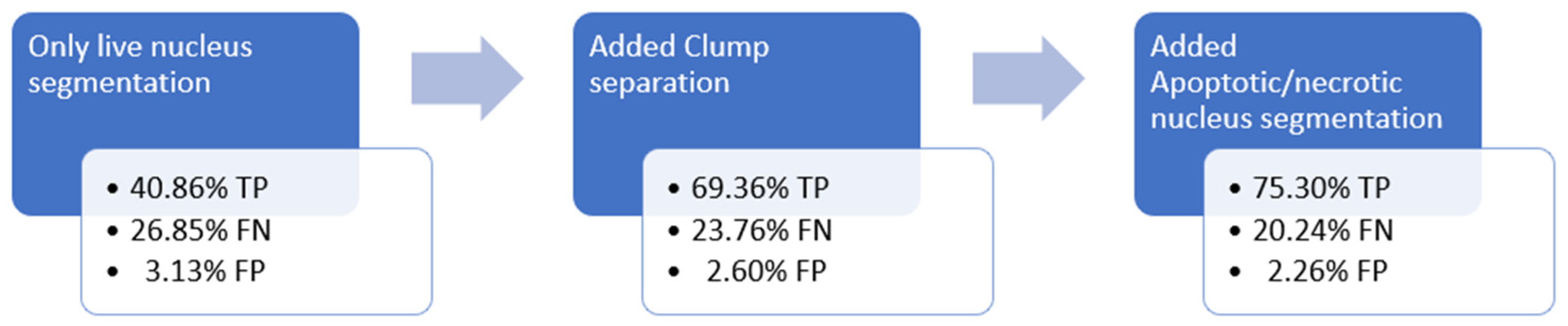
The first is the algorithm (our earlier proposal for the problem) described in [13,14,15,16]; it is a simple, threshold-based approach enhanced by a clump-splitting algorithm of our own development, similar in approach to [17], developed in the same period. The image pipeline consists of the initial nucleus segmentation, a step for clump separation and a step to enhance the ability of detecting low-intensity objects on the image.

Figure 4 shows the improvement in Algorithm 1 accuracy during the development process:

During the development of Algorithm 1, the polygon-to-polygon comparison type was used, with a homogeneous representation of the predictions, using half of the object radius as diameter, from the average object size calculated from all the samples [15]. If a single pixel overlap was present, it was considered a match [18]. In that part of the examination, the measurement and elimination of 1: n, m: 1 prediction-measurement matches. The goal during development was to follow a “test-driven” approach, so that changes made can be evaluated in a framework that produces comparable results.

2.4.2. Algorithm 2

The second method is a relatively advanced classical algorithm that utilizes adaptive thresholding. This local technique assesses each pixel and its surrounding neighborhood, computing the Gaussian mean of pixel intensities to classify the pixel. The image pipeline used in this method is illustrated in Figure 5 of the article [19].

2.4.3. Algorithm 3

The third algorithm chosen is a more modern, CNN-based algorithm. We chose to use StarDist [20] as the algorithm, and the pre-trained “2D_versatile_fluo” model included in the Python library. It has great advantages in separating staining anomalies from cell nuclei, by being constructed to segment round shapes; compared to Algorithm 1, which has no such integrated knowledge. Another aspect of this model is the diversity of the data it was trained on; multiple modalities and imaging techniques produced the input, which enhances segmentation robustness. For training our own model, we would need annotation data, of a polygonal type (in mask/label image representation); we plan to utilize these algorithms to consensually generate a ground truth and present the results in a different article.

The algorithms evaluated were selected based on their tractable behavior, which is important in clinical applications, their ability to handle the specific challenges of fluorescent sample analysis, and their computational efficiency, which is crucial for real-time diagnostic processes.

Initial evaluations of advanced approaches were carried out. Cellpose [21,22] performed well on fluorescent samples but was too computationally intensive for our use. Other options, such as HoVer-Net [23], U-Net [24], Mask R-CNN [25] and DeepLab v3+ [26], showed promise but require further comparison based on their computational demands and performance relative to the methods in this study. Our focus remained on how segmentation accuracy impacts population-based comparison to FCM results and the proposed calibration method.

2.5. Segmentation Validation: Matching, Counting

For the comparison to the manual, earlier, we used correlation-type metrics or a simple ratio of error classes to the whole population count [18]. For the current article, we did not need the depth and detail of that approach, so we opted to use a confusion matrix-based approach [27] to compare our segmentation algorithm candidates through sensitivity, precision and F1 score, as has been already successfully performed in [28].

The comparison is based on object-level matching between annotations and measurements, considering both representational and algorithmic options. Matching can involve reducing polygonal results to a single point for simple inclusion checks or assigning dimensions to landmark annotations for various matching methods. Figure 6 provides a visual summary of these techniques.

All the above are considered one-to-one assignments. It is possible to choose a more complex solution: registering multiple entities on either the annotations or on the object side (1:n, m:1). This can facilitate investigations of object clump splitting causing over- or undersegmentation, as was done during development of Algorithm 1 [15].

It is also possible to use more sophisticated, optimization-type methods (linear sum assignment problem [29,30]) for the matching, for example, minimizing the global cost function comprising of the distance sum of every pair.

2.6. Algorithm Comparison

For comparison of the algorithms in this article we chose the landmark-to-polygon method of simple inclusion. We followed the greedy method: the first match was registered, and the involved elements excluded from further matching.

We used a confusion matrix-based evaluation method, with the following model:

• TP: predicted location is included in the segmented object.
• FP: the segmented object does not include any predictions.
• FN: the prediction does not have any matches.
• TN: none.

Predictions only represent positive findings; where no predictions and no result are present, there is no useful information. There are many possible locations where there are no detected objects, and that is correct.

Because no TN values are available, specificity and negative predictive value is zero. Sensitivity, precision and F1 score can still be calculated.

2.6.1. Precision

This metric designates the algorithm’s strength in detecting only the relevant objects. It is also called positive predictive value (PPV):

$$\mathrm{Precision}=\mathrm{PPV}={\displaystyle \frac{\mathrm{TP}}{\mathrm{TP}+ \mathrm{FP}}}$$

(1)

The values produced by the algorithms for this metric can be found in second table of Section 3.1, with arithmetic mean and standard deviation values added.

2.6.2. Sensitivity

This value designates the algorithm’s strength in detecting all the relevant objects. It is also called recall, or true positive rate (TPR):

$$\mathrm{Sensitivity}=\mathrm{TPR}={\displaystyle \frac{\mathrm{TP}}{\mathrm{TP}+\mathrm{FN}}}$$

(2)

The values produced by the algorithms for this metric can be found in third table of Section 3.1, with arithmetic mean and standard deviation values added.

2.6.3. F1 Score

This score combines sensitivity and precision symmetrically (both are valued the same) in one metric:

$$\mathrm{F}1={\displaystyle \frac{2\mathrm{PPV}\times \mathrm{TPR}}{\mathrm{PPV}+\mathrm{TPR}}}={\displaystyle \frac{2\mathrm{TP}}{2\mathrm{TP}+\mathrm{FP}+\mathrm{FN}}}$$

(3)

Comparison of algorithms is done based on the calculated F1 scores. Using macro averaged F1 values for comparison is not advised according to [31]. A voting system can be set up, where a sample is considered a voter and votes for the best algorithm of the three, based on the F1 score achieved.

2.7. Population Level Comparison

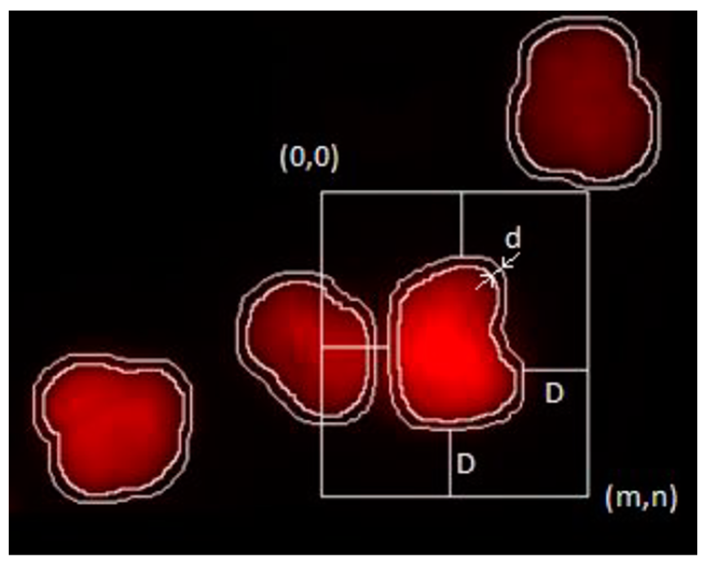
The segmented objects are used in the project for defining the region contributing to a nucleus. Features are extracted within this region to describe each data point contributing to a population-based evaluation. The most important is the integrated density (ID) for modeling DNA content. A schematic representation of how it is measured is visible in Figure 7. The FCM DNA histogram results are also available as a reference for each examined sample. This is the basis of the measurement of accuracy on the population level.

This measurement was conducted on a grayscale digital image, and in discrete format, as follows:

$$ID={{\displaystyle \sum }}_{i=j=1}^{i=m,j=n}((I_{m,n}\times J_{m,n})-\overline{BkgInt})$$

(4)

where ID is the integrated density, and I denotes the image intensities in the m, n neighborhood.

If O_i is the currently analyzed object:

$$O_i={\displaystyle \cup }{J}_{m,n}{I}_{m,n}$$

(5)

then J is an indicator function that has the value of 1 when it is a pixel corresponding to the measured object O_i, and 0 otherwise.

The neighborhood m, n was defined to ensure at least D distance from O_i. D was selected to be 35 pixels (the average object size in pixels at this magnification) so as to exclude other entire objects from the neighborhood; d was selected to be 5 pixels based on visual inspection (this is the distance where the bulk of the effect of object proximity is eliminated from intensity values).

We have shown that ID models the FCM method’s DNA content measurements well [9]. The nucleus populations identified in both datasets with the same process enables us to evaluate the difference that the segmentation algorithm change causes in the system. The mean values of the two populations of the DNA histogram of a healthy patient represent the 2n and 4n peaks. The peak ratio is the measured ratio of the DNA content at the 4n peak to the DNA content at the 2n peak. This theoretically equals 2.0 because, during mitosis, a normal body cell first replicates/doubles its DNA content before dividing into two new daughter cells. The location of these peaks showed great variance (even within the FCM result set), but the peak ratios show that the model parameters and the population classification are well defined.

Greater resemblance of these ratios to the ones measured on the FCM data means better overall performance.

For data manipulation and statistical evaluation, MATLAB (version R2019b) was used.

3. Results

3.1. Comparison of Algorithm Performance

We compared each algorithm to the ground truth in a pairwise fashion.

Table 1. F1 score for each sample and algorithm, with arithmetic mean and standard deviation over all the samples, calculated in a macroscopic manner.

Sample ID	Algorithm 1	Algorithm 2	Algorithm 3
1M01	0.8159	0.8817	0.8825
1M02	0.8076	0.8372	0.8440
1M03	0.8145	0.8270	0.8078
1M04	0.8468	0.8617	0.8423
1M06	0.8201	0.8480	0.8530
1M10	0.8502	0.8618	0.8920
1M11	0.8279	0.8583	0.8787
1M12	0.8065	0.8848	0.8718
1M13	0.8219	0.8488	0.8474
1M14	0.8041	0.8450	0.8351
1M15	0.6787	0.8265	0.7748
1M16	0.7929	0.8217	0.8214
1M17	0.8082	0.8271	0.8110
1M18	0.7708	0.8771	0.8523
1M20	0.8422	0.8278	0.8776
Mean	0.8072	0.8490 *	0.8461
SD	0.0397	0.0206 *	0.0314

* Algorithm 2 gave the most accurate result, along with more consistent results over the samples than the other two, but differences to Algorithm 3 are very small.

shows how the algorithms performed relative to each other, the comparison being based on the ground truth dataset.

In Figure 8, it can be seen how these algorithms are only slightly influenced by sample density (at least to the extent of this digital slide set).

Taking a second glance at Figure 8, sample 1M15 seems to be an outlier, and seemed useful to investigate. Figure 9 shows the main difference to the other samples. We intentionally selected an adjacent sample regarding density for comparison. Both samples are around average density, but most objects are in the groups visible on the image. These clumps are closely packed, and with the relatively high image intensity the objects are harder to separate. Sample intensity is also visibly different.

Table 2. Precision value for each sample and algorithm, with the arithmetic mean and standard deviation over all the samples, calculated in a macroscopic manner.

Sample ID	Algorithm 1	Algorithm 2	Algorithm 3
1M01	0.9564	0.8879	0.8706
1M02	0.9312	0.8773	0.8981
1M03	0.9148	0.7830	0.7866
1M04	0.9500	0.8773	0.8514
1M06	0.9315	0.8766	0.8785
1M10	0.9495	0.8269	0.8796
1M11	0.9517	0.8790	0.9153
1M12	0.9636	0.8823	0.8555
1M13	0.9477	0.8801	0.8713
1M14	0.9317	0.8744	0.8676
1M15	0.8409	0.8491	0.7954
1M16	0.9031	0.8494	0.8724
1M17	0.9448	0.8666	0.8767
1M18	0.8901	0.9018	0.8829
1M20	0.9628	0.7798	0.8792
Mean	0.9313	0.8594	0.8654
SD	0.0318	0.0352	0.0327

shows a comparison of the algorithms based on precision calculated from the confusion matrix. Algorithms 2 and 3 are close, but interestingly Algorithm 1 performs better than both.

Table 3. Sensitivity value for each sample and algorithm, with the arithmetic mean and standard deviation over all the samples, calculated in a macroscopic manner.

Sample ID	Algorithm 1	Algorithm 2	Algorithm 3
1M01	0.7114	0.8756	0.8948
1M02	0.7130	0.8007	0.7961
1M03	0.7341	0.8762	0.8301
1M04	0.7639	0.8465	0.8335
1M06	0.7325	0.8212	0.8290
1M10	0.7697	0.8997	0.9048
1M11	0.7327	0.8386	0.8449
1M12	0.6934	0.8872	0.8888
1M13	0.7255	0.8198	0.8248
1M14	0.7072	0.8175	0.8050
1M15	0.5689	0.8051	0.7552
1M16	0.7067	0.7959	0.7761
1M17	0.7062	0.7910	0.7545
1M18	0.6796	0.8536	0.8238
1M20	0.7485	0.8821	0.8761
Mean	0.7129	0.8407	0.8292
SD	0.0453	0.0353	0.0459

contains data for the sensitivity metric. In this regard, Algorithm 2 performs best of the three algorithms based on our findings.

Figure 10 shows the same sample region segmented by all the algorithms for better visibility of differences. See how each algorithm solves the segmentation on this somewhat problematic region.

Algorithms 2 and 3 are more sensitive to low-intensity nuclei, but produce false positives, due to the nature of the manually generated annotations. To compare the algorithms, we used their geometric data only. The task was to find a segmentation object pair for a reference marker. We executed the same matching algorithm for each of the three algorithms.

Algorithm 3 seems to follow object outlines best, resulting in more robust results from the validation point of view (markers are inside the segmentation objects by a greater margin). Clump separation is problematic with all three algorithms, but Algorithm 3 has further options for fine tuning in this regard. A few object clump separation cases are visible in Figure 11.

The calculated confusion matrix-based metrics are visible in

Table 4. Algorithm ranking based on micro-averaged F1 scores (calculated from the original confusion matrices) of each sample.

Rank	Algorithm 1	Algorithm 2	Algorithm 3
Mean Precision	0.9313	0.8594	0.8654
Mean Sensitivity	0.7129	0.8407	0.8292
Micro-averaged F1	0.8076	0.8499	0.8469
Macro-averaged F1	0.8072	0.8490	0.8461

. We used the micro-averaged F1 scores for the comparison(s).

Table 5. Ranked vote counts for algorithm evaluation. How many times an algorithm finished first, second and third regarding the F1 score in evaluating the samples.

Rank	Algorithm 1	Algorithm 2	Algorithm 3
#1	0	7	6
#2	3	7	8
#3	12	1	1

Only row #1 is used in the chosen voting model.

contains the counts used for the ranking of the algorithms. One of the options in defining the order of algorithms in performance can be defined based on these rank counts.

The algorithms show close performance to each other; we applied statistical methods to measure the significance of their differences. The natural choice would be the paired T test, but it is built upon assumptions that may not stand in the case of these datasets. The scores generated by Algorithm 1 cannot be considered to have normal distribution, based on the Shapiro-Wilk test (see Supplementary Materials). Because of this, and the small sample size, we chose the Wilcoxon Signed Rank test instead (see Supplementary Materials), that tolerates the low sample count better, does not build upon a normality assumption and tolerates outliers better. The pairwise comparisons (

Table 6. Results of the Wilcoxon Signed Rank test results (p-value). The test is symmetrical; only valuable data are presented.

	Algorithm 1	Algorithm 2	Algorithm 3
Algorithm 1		0.0003052	0.0006104
Algorithm 2			0.5614000
Algorithm 3

) show that there is a significant difference between A1 and the other two algorithms, but the difference between A2 and A3 is too small to call significant.

3.2. Comparison of Techniques

To measure the effect of algorithm performance on the technique’s ability to produce valid DNA histograms, we compared it to the FCM results.

The peak ratio is the ratio of the DNA content at the 4n peak to the DNA content of the 2n peak. This theoretically equals 2.0 because, during mitosis, a normal body cell first replicates/doubles its DNA content before dividing into two new daughter cells. The values measured by both techniques are visible in Figure 12 and

Table 7. Peak ratio properties of all the samples combined.

Population	Mean	SD
Algorithm 1	1.9349	0.039804
FCM	1.8868	0.022131
Algorithm 3	1.8894	0.034916

.

4. Discussion

There is significant improvement in object detection accuracy from Algorithm 1 to Algorithms 2 and 3, though the improvement is not consistent over all the samples (Figure 8). Macro-averaged F1 score, micro-averaged F1 score and the voting model are in consensus regarding the order of algorithms.

Looking at precision, Algorithm 1 performs better than Algorithms 2 and 3. In sensitivity, Algorithms 2 and 3 perform considerably better than Algorithm 1, comprising the differences visible in the F1 scores.

Visual inspection confirmed that Algorithms 2 and 3 perform better in two regards: clump separation and low-intensity object segmentation. Algorithm 2 is both more sensitive to darker objects and is a bit stronger in clump-handling than Algorithm 3; this results in the best F1 score of the three. During the creation of Algorithm 1, the clump separation module was a key step in creating an algorithm that would perform consistently on samples of different object densities. Algorithms 2 and 3 were intrinsically better in this regard: no performance decrease of notable measure was detected in relation to the density of objects on the samples, though Algorithm 3 could still be improved in this regard (there is possibility to fine-tune this behavior). Comparing the algorithms in this dimension might be part of a future investigation.

Interestingly, the complex but still classical method of Algorithm 2 performs best of the three on this sample set, though only very slightly—keeping in mind that Algorithm 3 can still be fine-tuned to this dataset (annotation with more information is needed).

It is important to note that clumps of objects are often comprised of objects of inhomogeneous intensities. It is also important to mention that low-intensity objects (on which Algorithms 2 and 3 perform significantly better) are usually apoptotic/necrotic cell nuclei that do not take part in the ploidy analysis result itself, and are filtered from the population during the later stages of the data analysis process.

Considering all the above: replacing Algorithm 1 with any of the other two is an improvement.

Based on the close results, the option for more fine-tuning and its extendibility, we chose Algorithm 3 to proceed to the population-level evaluation.

5. Conclusions

The results show that using more complex algorithms for this problem gives us better performance, but interestingly the increment is in the sensitivity measure. Precision was already high with even the simplest algorithm proposed by us a good few years ago. We were also able to show that the sample density, being an interesting factor in developing Algorithm 1, is less important for these more complex algorithms. They perform similarly across the samples in that regard (though we have seen cases where there is still room for improvement).

The results also show (Figure 12 and Table 7) that using a more accurate segmentation algorithm increases the accuracy (similarity to the reference FCM measurements) of results at the DNA histogram level.

Examining the samples #11 and #15, and comparing the algorithms regarding their accuracy in segmenting objects of different intensities is also something that could be worth pursuing, especially because during visual inspection multiple cases were encountered where the annotations were self-contradictory in the case of low-intensity objects.

Revision of the ground truth both in location and intensity might be considered based on the algorithms’ findings. Investigating the possibility to upgrade the ground truth data automatically, utilizing the segmentation results generated by multiple algorithms seems a challenging, though viable route for improvement.

While more complex algorithms such as U-Net, Mask R-CNN and DeepLab v3+ could potentially enhance segmentation accuracy, the available data may limit the achievable improvements (the non-significant difference between Algorithms 2 and 3 might be a precursor to this). There may be diminishing returns where increasing algorithm complexity yields only marginal accuracy gains, suggesting that the dataset itself—such as annotation quality or sample variability—may hinder further significant performance improvements, despite using more advanced models.

A focused study is needed to directly compare the (earlier) proposed calibration technique to current calibration practices, particularly using a greater number of samples. Such a study would provide more robust statistical validation of the system’s accuracy and reliability, helping to confirm its suitability for broader clinical adoption. By expanding the sample size and including various biological conditions, such research could better evaluate the technique’s effectiveness in real-world settings.

It is interesting to note that though annotation time took 20–40 min per sample depending on object count, all three algorithms took only seconds to run on the same region, having a clear time benefit. Adding that to the scanning time of a mean six and a half minutes (though the object segmentation step is only a part of the task), seems to be comparable to the reference technique.

References

1. McKinnon, K.M. Flow Cytometry: An Overview. Curr. Protoc. Immunol. 2018, 120, 5.1.1–5.1.11. [Google Scholar] [CrossRef] [PubMed]
2. Drescher, H.; Weiskirchen, S.; Weiskirchen, R. Flow Cytometry: A Blessing and a Curse. Biomedicines 2021, 9, 1613. [Google Scholar] [CrossRef]
3. Rakha, E.A.; Vougas, K.; Tan, P.H. Digital Technology in Diagnostic Breast Pathology and Immunohistochemistry. Pathobiology 2022, 89, 334–342. [Google Scholar] [CrossRef] [PubMed]
4. Ibrahim, A.; Gamble, P.; Jaroensri, R.; Abdelsamea, M.M.; Mermel, C.H.; Chen, P.-H.C.; Rakha, E.A. Artificial intelligence in digital breast pathology: Techniques and applications. Breast 2020, 49, 267–273. [Google Scholar] [CrossRef]
5. Braun, M.; Piasecka, D.; Bobrowski, M.; Kordek, R.; Sadej, R.; Romanska, H.M. A ‘Real-Life’ Experience on Automated Digital Image Analysis of FGFR2 Immunohistochemistry in Breast Cancer. Diagnostics 2020, 10, 1060. [Google Scholar] [CrossRef] [PubMed]
6. Gupta, A.; Harrison, P.J.; Wieslander, H.; Pielawski, N.; Kartasalo, K.; Partel, G.; Solorzano, L.; Suveer, A.; Klemm, A.H.; Spjuth, O.; et al. Deep Learning in Image Cytometry: A Review. Cytom. Part A 2019, 95, 366–380. [Google Scholar] [CrossRef]
7. Liang, Y.; Yin, Z.; Liu, H.; Zeng, H.; Wang, J.; Liu, J.; Che, N. Weakly Supervised Deep Nuclei Segmentation With Sparsely Annotated Bounding Boxes for DNA Image Cytometry. IEEE/ACM Trans. Comput. Biol. Bioinform. 2023, 20, 785–795. [Google Scholar] [CrossRef]
8. Ko, Y.S.; Choi, Y.M.; Kim, M.; Park, Y.; Ashraf, M.; Robles, W.R.Q.; Kim, M.-J.; Jang, J.; Yun, S.; Hwang, Y.; et al. Improving quality control in the routine practice for histopathological interpretation of gastrointestinal endoscopic biopsies using artificial intelligence. PLoS ONE 2022, 17, e0278542. [Google Scholar] [CrossRef]
9. Jónás, V.Z.; Paulik, R.; Kozlovszky, M.; Molnár, B. Calibration-Aimed Comparison of Image-Cytometry- and Flow-Cytometry-Based Approaches of Ploidy Analysis. Sensors 2022, 22, 6952. [Google Scholar] [CrossRef]
10. Kromp, F.; Bozsaky, E.; Rifatbegovic, F.; Fischer, L.; Ambros, M.; Berneder, M.; Weiss, T.; Lazic, D.; Dörr, W.; Hanbury, A.; et al. An annotated fluorescence image dataset for training nuclear segmentation methods. Sci. Data 2020, 7, 262. [Google Scholar] [CrossRef]
11. Cortacero, K.; McKenzie, B.; Müller, S.; Khazen, R.; Lafouresse, F.; Corsaut, G.; Van Acker, N.; Frenois, F.-X.; Lamant, L.; Meyer, N.; et al. Evolutionary design of explainable algorithms for biomedical image segmentation. Nat. Commun. 2023, 14, 7112. [Google Scholar] [CrossRef] [PubMed]
12. Roth, H.R.; Yang, D.; Xu, Z.; Wang, X.; Xu, D. Going to Extremes: Weakly Supervised Medical Image Segmentation. Mach. Learn. Knowl. Extr. 2021, 3, 507–524. [Google Scholar] [CrossRef]
13. Jonas, V.Z.; Kozlovszky, M.; Molnar, B. Ploidy analysis on digital slides. In Proceedings of the CINTI 2013—14th IEEE International Symposium on Computational Intelligence and Informatics, Budapest, Hungary, 19–21 November 2013. [Google Scholar] [CrossRef]
14. Jonas, V.Z.; Kozlovszky, M.; Molnar, B. Nucleus detection on propidium iodide stained digital slides. In Proceedings of the SACI 2014—9th IEEE International Symposium on Applied Computational Intelligence and Informatics, Proceedings, Timisoara, Romania, 15–17 May 2014. [Google Scholar] [CrossRef]
15. Jonas, V.Z.; Kozlovszky, M.; Molnar, B. Separation enhanced nucleus detection on propidium iodide stained digital slides. In Proceedings of the INES 2014—IEEE 18th International Conference on Intelligent Engineering Systems, Tihany, Hungary, 3–5 July 2014. [Google Scholar] [CrossRef]
16. Jonas, V.Z.; Kozlovszky, M.; Molnar, B. Detecting low intensity nuclei on propidium iodide stained digital slides. In Proceedings of the CINTI 2014—15th IEEE International Symposium on Computational Intelligence and Informatics, Budapest, Hungary, 19–21 November 2014. [Google Scholar] [CrossRef]
17. Samsi, S.; Trefois, C.; Antony, P.M.A.; Skupin, A. Automated nuclei clump splitting by combining local concavity orientation and graph partitioning. In Proceedings of the 2014 IEEE-EMBS International Conference on Biomedical and Health Informatics, BHI 2014, Valencia, Spain, 1–4 June 2014; pp. 412–415. [Google Scholar] [CrossRef]
18. Jonas, V.Z.; Kozlovszky, M.; Molnar, B. Semi-automated quantitative validation tool for medical image processing algorithm development. In Proceedings of the Technological Innovation for Cloud-Based Engineering Systems: 6th IFIP WG 5.5/SOCOLNET Doctoral Conference on Computing, Electrical and Industrial Systems, DoCEIS 2015, Costa de Caparica, Portugal, 13–15 April 2015; Volume 450. [Google Scholar] [CrossRef]
19. Paulik, R.; Micsik, T.; Kiszler, G.; Kaszál, P.; Székely, J.; Paulik, N.; Várhalmi, E.; Prémusz, V.; Krenács, T.; Molnár, B. An optimized image analysis algorithm for detecting nuclear signals in digital whole slides for histopathology. Cytom. Part A 2017, 91, 595–608. [Google Scholar] [CrossRef] [PubMed]
20. Schmidt, U.; Weigert, M.; Broaddus, C.; Myers, G. Cell detection with star-convex polygons. In Lecture Notes in Computer Science, Proceedings of the Medical Image Computing and Computer Assisted Intervention–MICCAI 2018: 21st International Conference, Granada, Spain, 16–20 September 2018; Springer: Cham, Switzerland, 2018. [Google Scholar] [CrossRef]
21. Stringer, C.; Wang, T.; Michaelos, M.; Pachitariu, M. Cellpose: A generalist algorithm for cellular segmentation. Nat. Methods 2021, 18, 100–106. [Google Scholar] [CrossRef] [PubMed]
22. Pachitariu, M.; Stringer, C. Cellpose 2.0: How to train your own model. Nat. Methods 2022, 19, 1634–1641. [Google Scholar] [CrossRef]
23. Graham, S.; Vu, Q.D.; Raza, S.E.A.; Azam, A.; Tsang, Y.W.; Kwak, J.T.; Rajpoot, N. Hover-Net: Simultaneous segmentation and classification of nuclei in multi-tissue histology images. Med. Image Anal. 2019, 58, 101563. [Google Scholar] [CrossRef]
24. Ronneberger, O.; Fischer, P.; Brox, T. U-net: Convolutional networks for biomedical image segmentation. In Lecture Notes in Computer Science, Proceedings of the Medical Image Computing and Computer-Assisted Intervention–MICCAI 2015: 18th International Conference, Munich, Germany, 5–9 October 2015; Springer: Cham, Switzerland, 2015. [Google Scholar] [CrossRef]
25. He, K.; Gkioxari, G.; Dollár, P.; Girshick, R. Mask R-CNN. IEEE Trans. Pattern Anal. Mach. Intell. 2020, 42, 386–397. [Google Scholar] [CrossRef]
26. Chen, L.C.; Zhu, Y.; Papandreou, G.; Schroff, F.; Adam, H. Encoder-decoder with atrous separable convolution for semantic image segmentation. In Proceedings of the European Conference on Computer Vision (ECCV), Munich, Germany, 8–14 September 2018. [Google Scholar] [CrossRef]
27. Tharwat, A. Classification assessment methods. Appl. Comput. Inform. 2018, 17, 168–192. [Google Scholar] [CrossRef]
28. Janowczyk, A.; Madabhushi, A. Deep learning for digital pathology image analysis: A comprehensive tutorial with selected use cases. J. Pathol. Inform. 2016, 7, 29. [Google Scholar] [CrossRef]
29. Singh, S. A Comparative Analysis of Assignment Problem. IOSR J. Eng. 2012, 2, 1–15. [Google Scholar] [CrossRef]
30. Virtanen, P.; Gommers, R.; Oliphant, T.E.; Haberland, M.; Reddy, T.; Cournapeau, D.; Burovski, E.; Peterson, P.; Weckesser, W.; Bright, J.; et al. SciPy 1.0: Fundamental Algorithms for Scientific Computing in Python. Nat. Methods 2020, 17, 261–272. [Google Scholar] [CrossRef] [PubMed]
31. Zhang, D.; Wang, J.; Zhao, X. Estimating the uncertainty of average F1 scores. In Proceedings of the ICTIR 2015—Proceedings of the 2015 ACM SIGIR International Conference on the Theory of Information Retrieval, New York, NY, USA, 27–30 September 2015. [Google Scholar] [CrossRef]
Figure 1. The current state of the project that is the greater environment of this study. Creating an ICM-based approach to parallel flow cytometry regarding ploidy analysis, with option for calibration.
Applsci 14 08707 g001
Figure 2. Schematic representation of the project this investigation is part of. The topic of this article is highlighted in blue.
Applsci 14 08707 g002
Figure 3. The process of validation from left to right. The same annotation set was used as a reference for all three algorithms.
Applsci 14 08707 g003
Figure 4. Algorithm 1 was developed as a modular image processing pipeline. From left to right the modules developed are visualized. The relative values of TP, FN, and FP to the count of segmented objects achieved after adding the module are also listed.
Applsci 14 08707 g004
Figure 5. Flow chart diagram illustrating the modular framework of the cell nucleus-detection algorithm. (a) source: true color brightfield or fluorescent (RGB or grayscale) stained image; (b) nuclei channel extraction; (c) adaptive thresholding; (d–g) algorithm steps of the hole filling method; (h) distance transformation; (i) nuclear seed detection; (j) segment labeling; (k) watershed region growing and object separation; (l) label smoothing; (m) label filtering; (n) final results.
Applsci 14 08707 g005
Figure 6. Annotation-segmentation matching options: (a) landmark-to-landmark, (b) landmark-to-polygon, (c) polygon-to-polygon (intersection), (d) polygon-to-polygon (Jaccard). X-es designate the landmark locations: in yellow or (m, M) the marker/annotation representations, shapes in blue (O, A1 and c) are the corresponding object representation. Pixel set operation results (intersection, union) in purple.
Applsci 14 08707 g006
Figure 7. Method of measuring integrated density (ID), a background-compensated intensity sum. The resolution of the system is visible; the objects are only tens of pixels in size.
Applsci 14 08707 g007
Figure 8. The F1 scores are calculated from the confusion matrices calculated for each algorithm, for each sample. The horizontal axis values are in increasing order of sample density and a normalized value of this is also present on the chart (dashed green, with rectangular data points). F1 score decreases only slightly with increasing density in the case of all three algorithms.
Applsci 14 08707 g008
Figure 9. Region exported from sample 1M11 (left) and 1M15 (right) to show cause of relatively bad segmentation metrics: object clumping.
Applsci 14 08707 g009
Figure 10. Segmentation results of Algorithms 1 (blue), 2 (white), 3 (red) respectively from left to right on the same region. Yellow spots are hand-placed annotations. Algorithms 2 and 3 are visibly more sensitive to weakly stained objects, with this also producing more false positive finds.
Applsci 14 08707 g010
Figure 11. Samples from the segmentation results of Algorithms 1 (blue) and 3 (red) on the same regions. Thresholding is inferior in segmenting exact object boundaries due to lack of information that the objects are round (a). This information also aids in the separation of clumps (b). In some cases even over-segmentation can be avoided on the same basis ((c) bottom center). On the other hand, it can cause problems when the goal is to count dividing nuclei; separating them into two cells can ruin the foundation of the measurement method (d).
Applsci 14 08707 g011aApplsci 14 08707 g011b
Figure 12. Graphical comparison of Algorithms 1 (blue) and 3 (red) to the FCM (green) reference. The peak ratios for the 15 samples in two equivalent representations; the datasets are marked with the same color on both plots.
Applsci 14 08707 g012