Author Contributions
Investigation, C.L.; methodology, T.D.; software, T.D. and S.H. (Shishuo Han); supervision, H.X.; validation, C.L. and S.H. (Shishuo Han); writing—original draft, T.D. and S.H. (Song Huang); writing—review and editing, G.H. All authors have read and agreed to the published version of the manuscript.
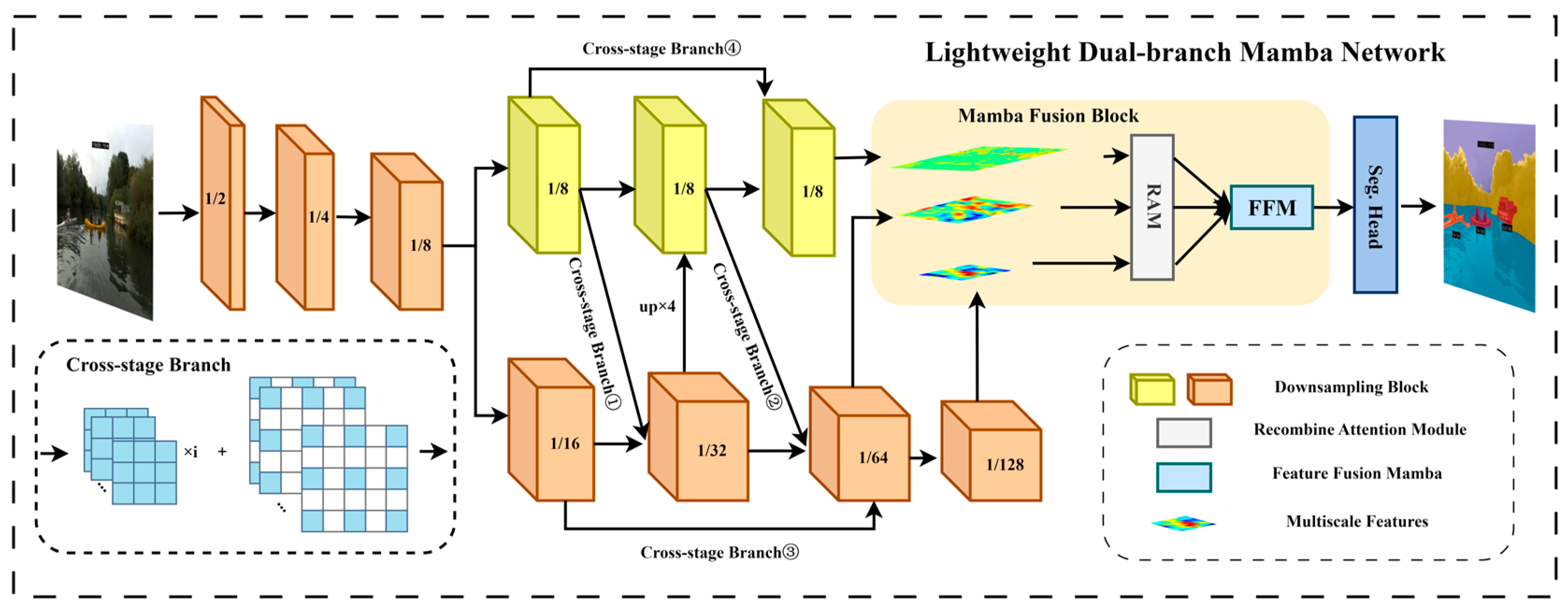
Figure 1.
The overall architecture of LDMNet, including the Mamba Fusion Block and the detailed structure of the cross-stage fusion branches. The notations such as ½ and 1/4 represent the downsampling multiples of the feature maps by the residual basic blocks. RAM denotes the Recombine Attention Module, FFM stands for Feature Fusion Mamba, and Seg. Head refers to the segmentation head. The detailed structure of the Cross-stage Branch is depicted within the dashed box.
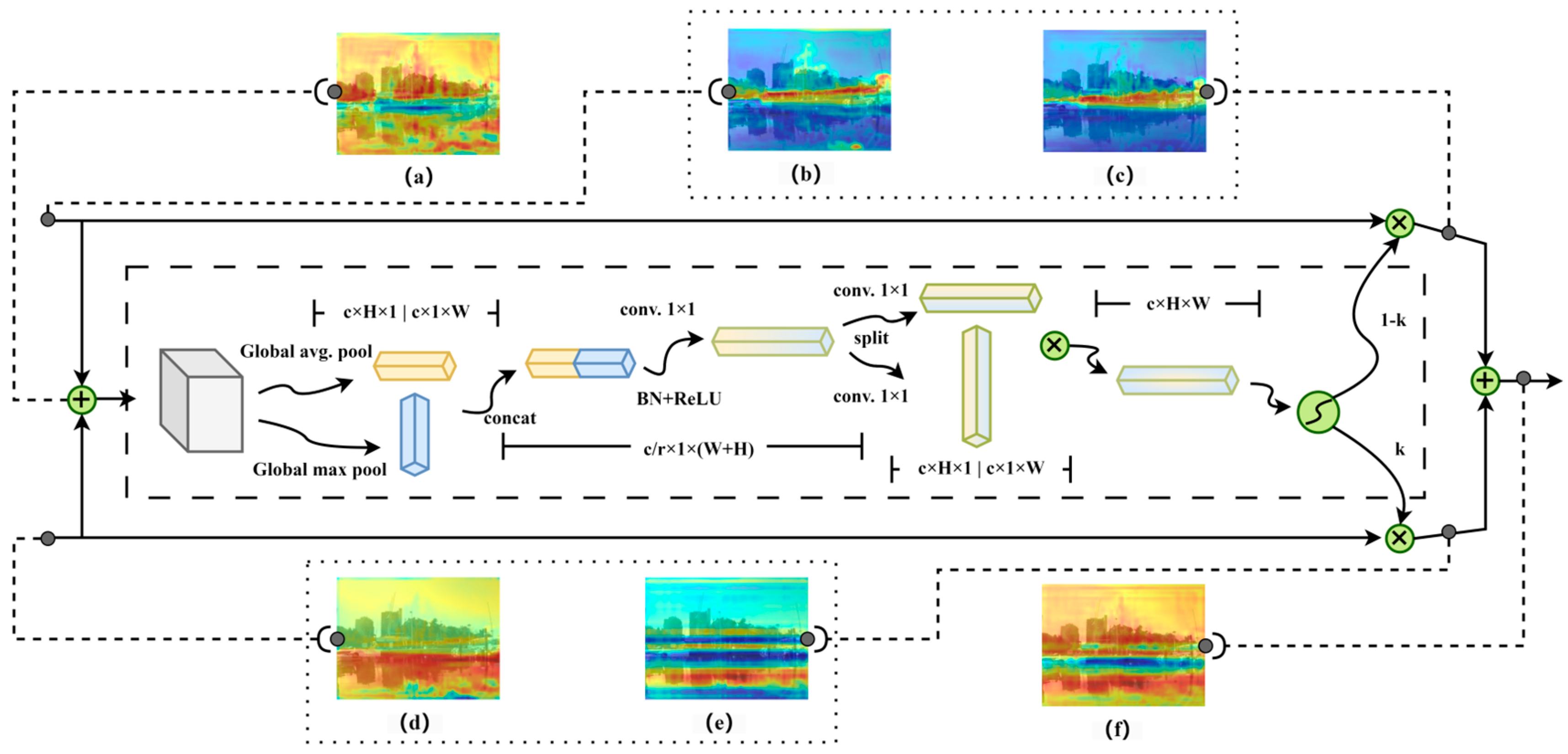
Figure 2.
Schematic diagram of the Recombine Attention Module (RAM) structure. In the diagram, the spatial dimensions of the feature maps at each stage are indicated. The images within the dashed boxes represent intermediate process feature maps, which are connected to the corresponding positions in the RAM with dashed lines. The two input branches on the left represent the input feature maps with high-resolution differences, corresponding to feature maps (b,d). After processing, the feature maps of each branch can be compared with (b) and (d) by (c) and (e), respectively. The feature maps after passing through the RAM can be compared with (a,f).
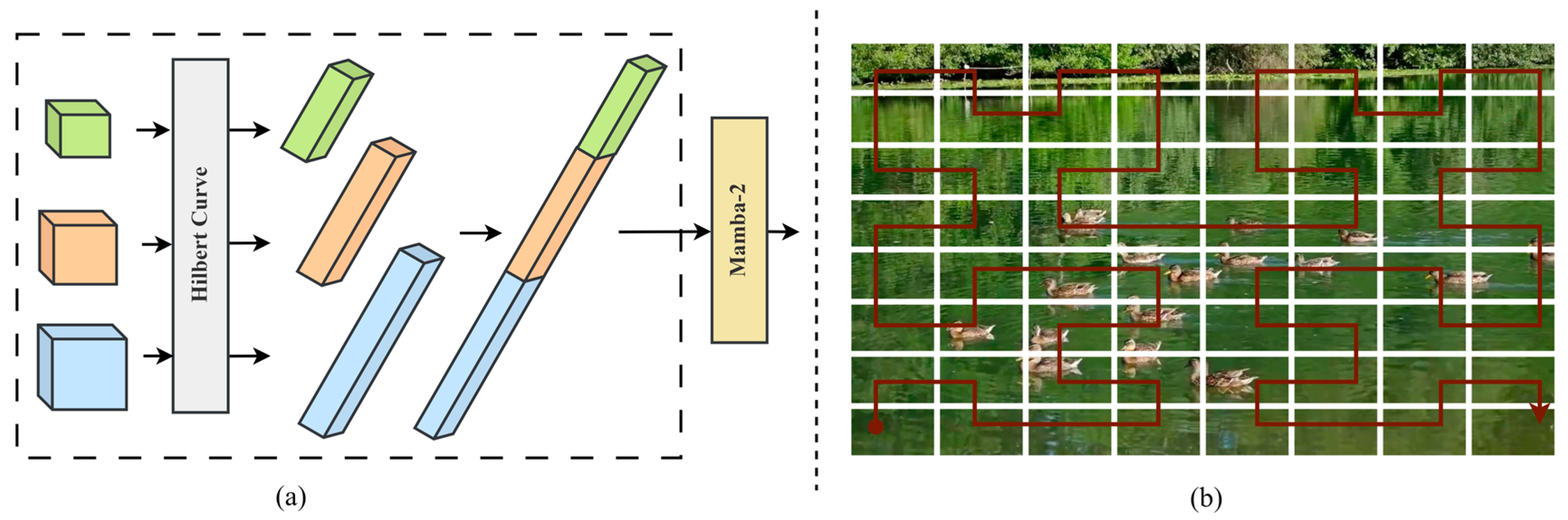
Figure 3.
Illustrates the operation of the Feature Fusion Mamba (FFM). In (a), the detailed structure of the FFM is shown, where Hilbert Curve represents the use of the Hilbert curve as the traversal path for serializing the spatial arrangement of patch sequences. (b) The Hilbert curve traversal path.
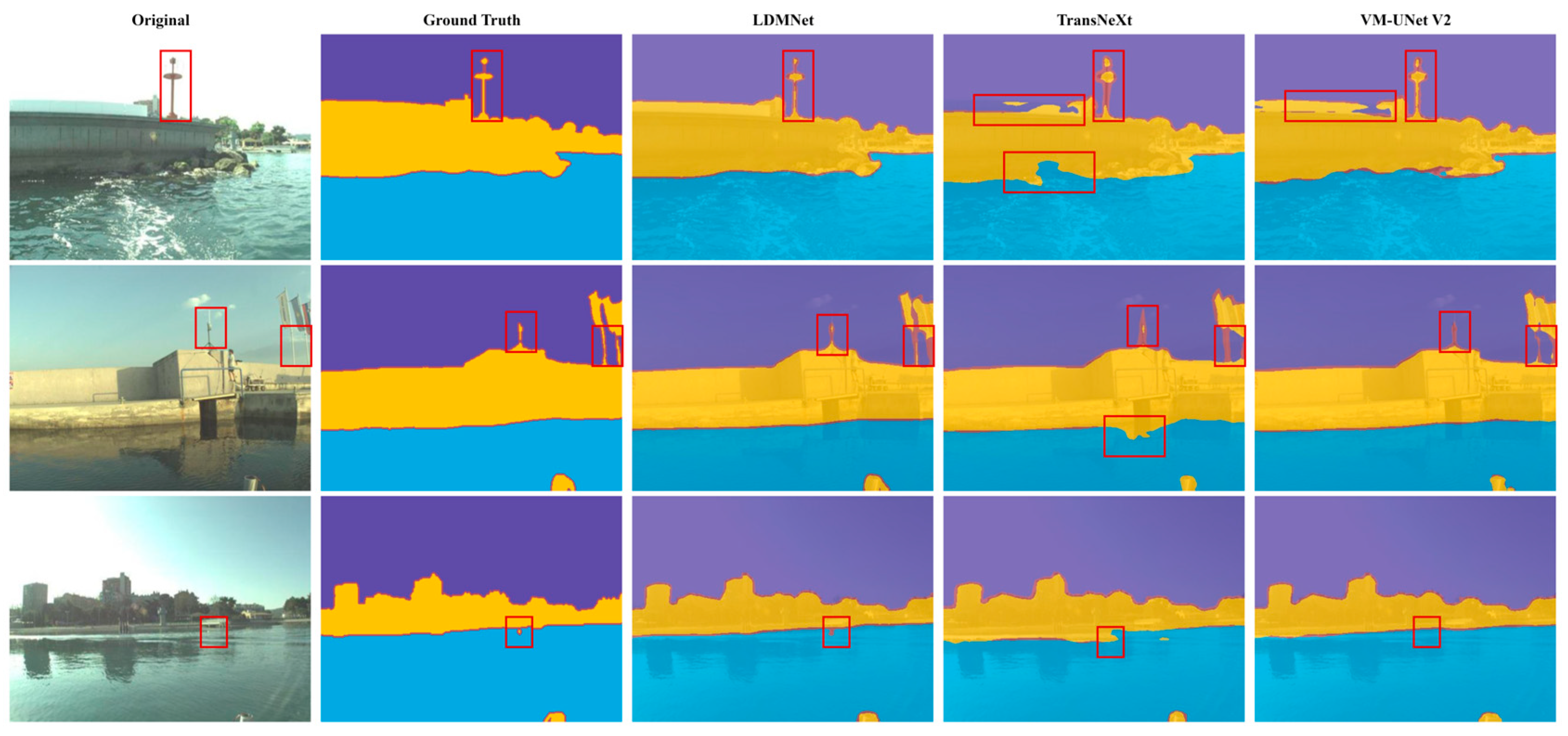
Figure 4.
Visualization of the inference of LDMNet compared to TransNeXt [
53] and VM-UNet V2 [
15] on the MaSTr1325 for close-up targets. We have marked the detailed differences with red boxes.
Figure 4.
Visualization of the inference of LDMNet compared to TransNeXt [
53] and VM-UNet V2 [
15] on the MaSTr1325 for close-up targets. We have marked the detailed differences with red boxes.
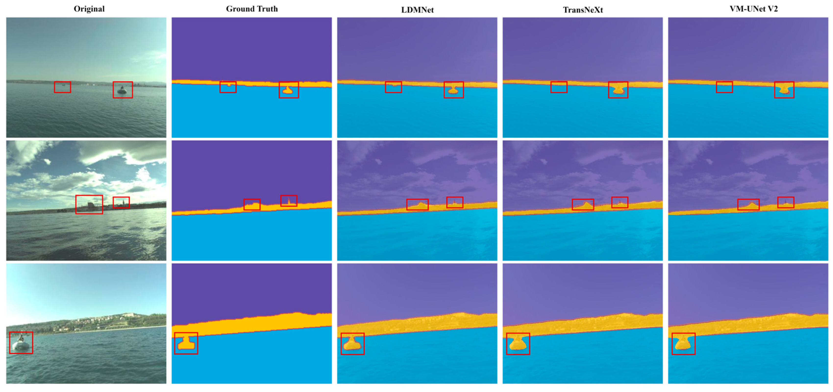
Figure 5.
Visualization of the inference of LDMNet compared to TransNeXt and VM-UNet V2 on the MaSTr1325 for distant targets. We have marked the detailed differences with red boxes.
Figure 5.
Visualization of the inference of LDMNet compared to TransNeXt and VM-UNet V2 on the MaSTr1325 for distant targets. We have marked the detailed differences with red boxes.
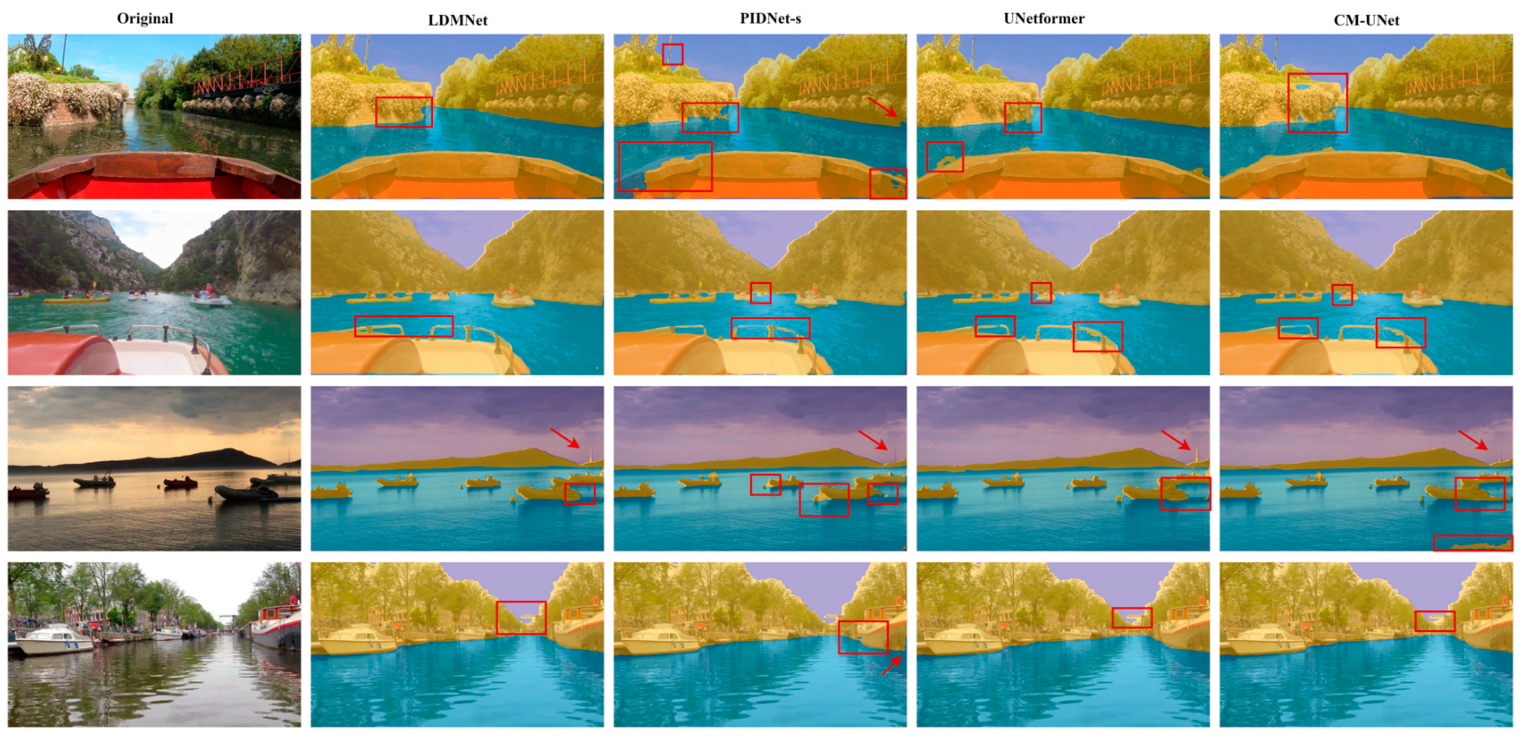
Figure 6.
Visualization of the inference of PIDNet-s, UNetformer, CM-UNet, and LDMNet on the LaRS. We have marked the detailed differences with red boxes and red arrows.
Figure 6.
Visualization of the inference of PIDNet-s, UNetformer, CM-UNet, and LDMNet on the LaRS. We have marked the detailed differences with red boxes and red arrows.
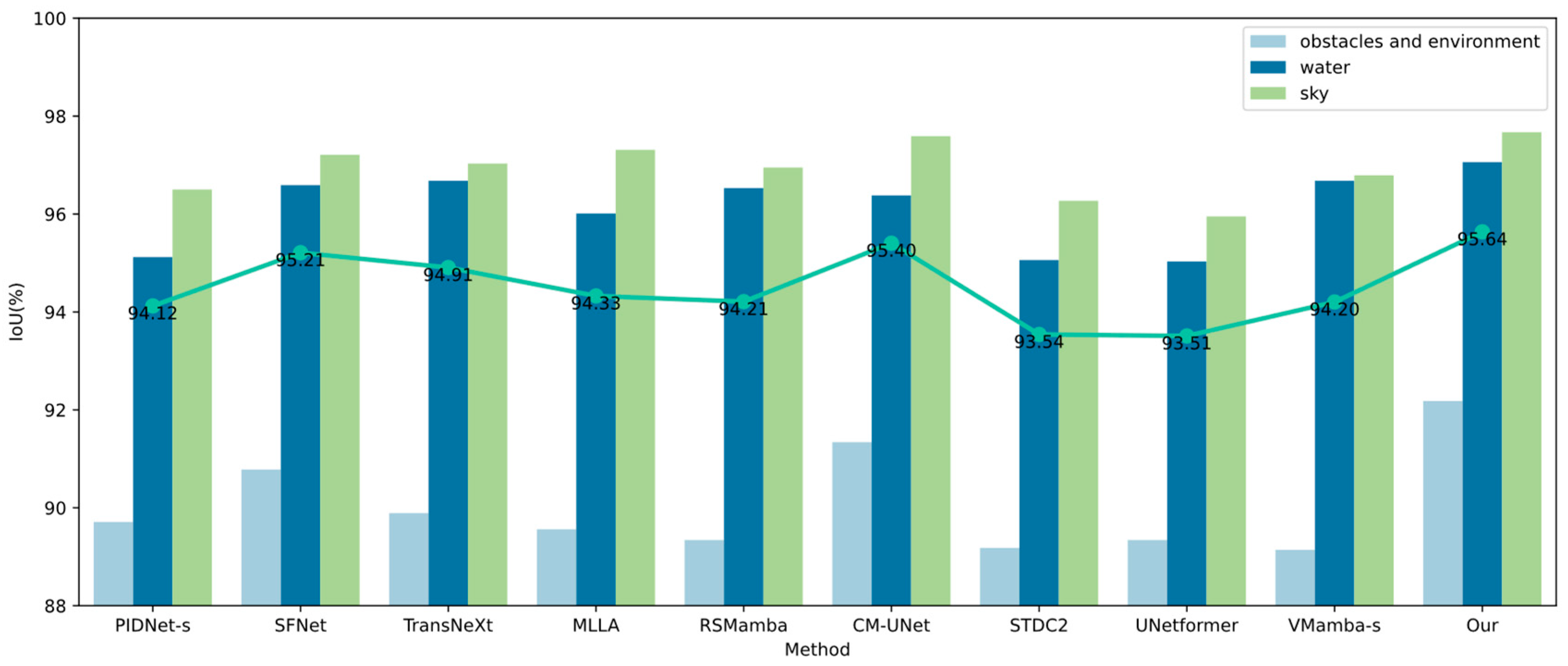
Figure 7.
Comparison of the IoU of different methods in predicting various categories on the LaRS. Among them, the green solid line with circles indicates the mIoU difference between different models on LaRS.
Figure 7.
Comparison of the IoU of different methods in predicting various categories on the LaRS. Among them, the green solid line with circles indicates the mIoU difference between different models on LaRS.
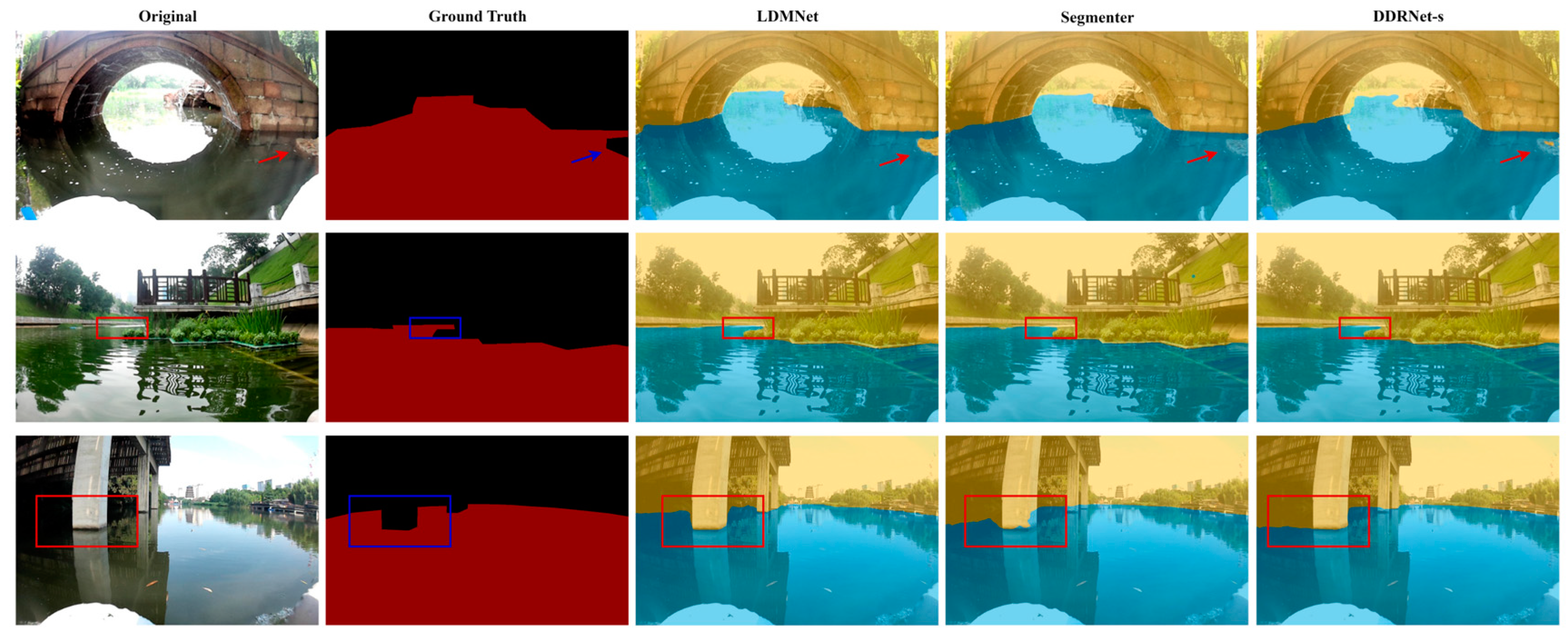
Figure 8.
Visualizes the inference of LDMNet compared to BisenetV2 and DDRNet-s on the Water Segmentation in the USVInland for water–shore segmentation. We have marked the detailed differences with boxes and arrows. It can be seen that in complex environments where the reflection of the water surface is overcome, LDMNet still demonstrates high accuracy in demarcating the boundaries between the water and the shore.
Table 1.
Parameters of the Cross-stage Branch in LDMNet. It can be observed that we employ four different fusion methods, and each one concludes with a 1 × 1 convolution for channel compression. To increase the receptive field, we incorporate Atrous convolutions in the first three types of cross-stage fusions.
| Branch Name | Cross-Stage Branch in LDMNet Setting |
|---|
| | Kernel (Size/Stride/Padding) | Channels | Dilation Rate | Repeating Times |
|---|
| Cross-stage Branch ① | 3 × 3/2/1 | 64 | 1 | x = 1 |
| 3 × 3/2/2 | 256 | 2 | x = 1 |
| 1 × 1 | 512 | - | x = 1 |
| Cross-stage Branch ② | 3 × 3/2/1 | 64/256 | 1 | x = 2 |
| 3 × 3/2/2 | 512 | 2 | x = 1 |
| 1 × 1 | 1024 | - | x = 1 |
| Cross-stage Branch ③ | 3 × 3/2/1 | 128 | s1 | x = 1 |
| 3 × 3/2/2 | 512 | 2 | x = 1 |
| 1 × 1 | 1024 | - | x = 1 |
| Cross-stage Branch ④ | 3 × 3/1/1 | 64 | 1 | x = 1 |
| 1 × 1 | 256 | - | x = 1 |
Table 2.
Important parameters of the datasets used.
Table 2.
Important parameters of the datasets used.
| Dataset | Type | Train | Val. | Resolution | Class |
|---|
| MaSTr1325 | Marine Obstacle Segmentation | 1060 | 265 | 512 × 512 | 3 |
| LaRS | Marine Obstacle Segmentation | 2605 | 198 | 1024 × 1024 | 3 |
| Water Segmentation | Distinguishing between Reflections and the Actual Division of Water and Land | 1166 | 234 | 640 × 640 | 2 |
| Cityscapes | Semantic Segmentation of Cityscapes | 2975 | 500 | 1024 × 1024 | 19 |
Table 3.
Accuracy comparison of LDMNet with other advanced methods on MaSTr1325. Among them, "-" indicates a lack of relevant data.
Table 3.
Accuracy comparison of LDMNet with other advanced methods on MaSTr1325. Among them, "-" indicates a lack of relevant data.
| Model | Type | GPU | Resolution | Params ↓ | mIoU (%) ↑ | Speed (FPS) ↑ |
|---|
| Deeplab V3+ [22] | CNN | V100 | 512 × 512 | - | 85.4 | 0.56 |
| SegNet [23] | CNN | V100 | 512 × 512 | - | 81.8 | 0.85 |
| WODIS [52] | CNN | V100 | 512 × 384 | 89.5 M | 91.3 | 43.2 |
| Fast SCNN [25] | CNN | 3070Ti | 512 × 512 | 1.36 M | 93.5 | 67.5 |
| DDRNet-s [8] | CNN | 3070Ti | 512 × 512 | 17.05 M | 94.5 | 79 |
| Segmenter(vit-s) [24] | Transformer | 3070Ti | 512 × 512 | - | 94.8 | 53.4 |
| TransNeXt-t [53] | Transformer | 4090Ti | 512 × 512 | 28.2 M | 95.4 | 10.3 |
| UNetformer(R18) [20] | Transformer | 3070Ti | 512 × 512 | 11.69 M | 94.2 | 5.6 |
| VMamba-s [13] | Mamba | 3070Ti | 512 × 512 | 70 M | 93.6 | 52 |
| VM-UNet [14] | Mamba | 3070Ti | 512 × 512 | 34.62 M | 93.4 | 21.1 |
| VM-UNetV2 [15] | Mamba | 3070Ti | 512 × 512 | 17.91 M | 94.8 | 32 |
| CM-UNet [16] | Mamba | 3070Ti | 512 × 512 | 12.89 M | 93.7 | 8.5 |
| LDMNet | CNN&Mamba | 3070Ti | 512 × 512 | 12.53 M | 96.2 | 80 |
Table 4.
Accuracy comparison of LDMNet with other advanced methods on LaRS.
Table 4.
Accuracy comparison of LDMNet with other advanced methods on LaRS.
| Model | Type | mIoU (%) ↑ | Re (%) ↑ | F1 ↑ |
|---|
| ICNet [54] | CNN | 93.3 | 49.7 | 44.9 |
| STDC2 [55] | CNN | 93.5 | 54.3 | 54.3 |
| PiDNet-s [7] | CNN | 94.1 | 61.8 | 52.2 |
| SFNet [56] | CNN | 95.2 | 62.4 | 58.1 |
| Segmenter [24] | Transformer | 95.1 | 59.5 | 55.2 |
| MLLA [19] | Transformer | 95.3 | 63.5 | 59.4 |
| UNetformer [20] | Transformer | 93.5 | 61.5 | 54.3 |
| TransNeXt-t [53] | Transformer | 94.9 | 61.3 | 53.1 |
| RSMamba [57] | Mamba | 94.2 | 60.1 | 52.9 |
| VM-UNet [14] | Mamba | 95.1 | 64.2 | 61.3 |
| CM-UNet [16] | Mamba | 95.4 | 65.4 | 62.8 |
| VMamba-s [13] | Mamba | 94.2 | 60.5 | 54.2 |
| LDMNet | CNN&Mamba | 95.6 | 78.6 | 75.2 |
Table 5.
Accuracy comparison of LDMNet with other advanced methods on Water Segmentation in the USVInland.
Table 5.
Accuracy comparison of LDMNet with other advanced methods on Water Segmentation in the USVInland.
| Model | Resolution | mIoU (%) ↑ | mDice (%) ↑ |
|---|
| BisenetV2 [58] | 640 × 640 | 97.68 | 98.46 |
| DDRNet-s [8] | 640 × 640 | 98.64 | 99.15 |
| Segmenter(vit-s) [24] | 640 × 640 | 98.80 | 99.23 |
| LDMNet | 640 × 640 | 99.02 | 99.51 |
Table 6.
Accuracy comparison of LDMNet with other advanced methods on Cityscapes. Among them, "-" indicates a lack of relevant data.
Table 6.
Accuracy comparison of LDMNet with other advanced methods on Cityscapes. Among them, "-" indicates a lack of relevant data.
| Model | Resolution | mIoU (%) ↑ | GFLOPs ↓ |
|---|
| SFNet(DF1) [56] | 2048 × 1024 | 74.5 | 24.7 |
| STDC2-Seg75 [55] | 1536 × 768 | 76.8 | - |
| PP-LiteSeg-T2 [9] | 1536 × 768 | 74.9 | - |
| HyperSeg-M [30] | 1024 × 512 | 75.8 | 7.5 |
| PIDNet-S [7] | 2048 × 1024 | 77.1 | 46.3 |
| DDRNet-s [8] | 2048 × 1024 | 77.2 | 34.2 |
| LDMNet | 2048 × 1024 | 80.7 | 32.9 |
Table 7.
Comparison of the number of parameters between RAM and AFF [
28], showing that RAM has fewer parameters than AFF.
Table 7.
Comparison of the number of parameters between RAM and AFF [
28], showing that RAM has fewer parameters than AFF.
| Method | Params |
|---|
| AFF [28] | 39.71 k |
| RAM | 39.58 k |
Table 8.
Comparison of the enhancement effects of RAM and AFF [
28] on different Backbones on MaSTr1325, where SS represents the Sequential Scan Module, SS2D [
53] denotes the 2D Selective Scan Module, and OSSM [
57] signifies the Omnidirectional Selective Scan Module. δ is the change obtained by subtracting the corresponding items of AFF from RAM, with DDRNet + Mamba (SS) as the comparison object. "-" indicates that the current row is used as the baseline.
| Method | mIoU (%) ↑ | mPA (%) ↑ | δ |
|---|
| DDRNet + Mamba | δ (mIoU) (%) ↑ | δ (mPA) (%) ↑ |
|---|
| +SS | | | | | |
| | +AFF | 92.53 | 94.97 | - | - |
| | +RAM | 93.87 (+1.34) | 95.56 (+0.59) | +1.34 | +0.59 |
| +SS2D [53] | | | | | |
| | +AFF | 93.09 | 94.68 | −0.56 | −0.29 |
| | +RAM | 94.23 (+1.14) | 95.34 (+0.66) | +0.36 | −0.22 |
| +OSSM [57] | | | | | |
| | +AFF | 93.04 | 94.37 | +0.51 | −0.60 |
| | +RAM | 94.42 (+1.38) | 95.48 (+1.11) | +0.55 | −0.08 |
| +HCS | | | | | |
| | +AFF | 94.68 | 97.02 | +2.15 | +2.05 |
| | +RAM | 95.96 (+1.28) | 97.68 (+0.66) | +2.09 | +2.12 |
| LDMNet + Mamba | | | | |
| +SS | | | | | |
| | +AFF | 93.43 | 95.42 | +0.90 | +0.45 |
| | +RAM | 94.12 (+0.69) | 95.80 (+0.38) | +0.25 | +0.24 |
| +SS2D [53] | | | | | |
| | +AFF | 94.17 | 95.94 | +1.64 | +0.97 |
| | +RAM | 95.34 (+1.17) | 96.84 (+0.90) | +1.47 | +1.28 |
| +OSSM [57] | | | | | |
| | +AFF | 94.47 | 96.02 | +1.94 | +1.05 |
| | +RAM | 95.06 (+0.59) | 96.51 (+0.49) | +1.19 | +0.95 |
| +HCS | | | | | |
| | +AFF | 95.32 | 97.38 | +2.79 | +2.41 |
| | +RAM | 96.16 (+0.84) | 97.92 (+0.54) | +2.29 | +2.36 |
Table 9.
Ablation experiments of LDMNet on MaSTr1325. Among them, "✓" indicates that this module is retained, while "✗" indicates the opposite.
Table 9.
Ablation experiments of LDMNet on MaSTr1325. Among them, "✓" indicates that this module is retained, while "✗" indicates the opposite.
| +RAM | +HCS | +Mamba-2 | mIoU (%) ↑ | mPA (%) ↑ |
|---|
| ✗ | ✗ | ✗ | 94.56 | 96.77 |
| ✓ | ✗ | ✗ | 95.43 | 97.04 |
| ✗ | ✗ | ✓ | 95.52 | 97.16 |
| ✗ | ✓ | ✓ | 95.78 | 97.56 |
| ✓ | ✗ | ✓ | 96.09 | 97.80 |
| ✓ | ✓ | ✓ | 96.16 | 97.92 |


