Determining the Head Characteristics of Radial Centrifugal Pumps under the Impact of Prewhirl

Abstract

The flow rate is a significant factor in the operation of centrifugal pumps. The characteristic curve of the pump head is frequently employed in the calculation of the flow rate. Nevertheless, this may be subject to alteration because of prewhirl on the suction side of the pump. Calculating the changes in the head’s characteristic curve reveals a change in hydraulic losses. The impact of prewhirl on hydraulic losses is investigated by experimental and numerical analysis of two radial centrifugal pumps. It is demonstrated that the primary changes occur in the pump impeller losses. Relative velocity is a significant factor in this context. Alterations in the pumps’ configurations result in a range of secondary flows and shock losses at the leading edge of the blades. A physical model, derived on the basis of the relative velocity, is used to predict the characteristic curves of radial centrifugal pumps with prewhirl with a high degree of accuracy. The results demonstrate a notable enhancement in comparison to modelling techniques that do not incorporate the fluctuating hydraulic losses.

1. Introduction

Centrifugal pumps are widely applicable in fields ranging from the energy industry to wastewater treatment. Pumps are used to generate a flow rate, which needs to be adapted to the requirements of the specific application using one of various possible control methods. In particular, the flow rate is considered the main control variable in many applications, e.g., in the process industry [1,2] and is a significant factor in optimising pump operation. The operating point of the pump can be determined based on corresponding information. A large number of publications have already addressed the issue of determining the flow rate of centrifugal pumps using soft sensors. S. Leonow gave an overview of the most common approaches of flow rate estimation [1]. These approaches can be divided into static and dynamic methods [1]. Depending on the kind of estimation approach, the measured values either of the head or the power consumption of the pump are required as input parameters of the empirical equations for deriving the flow rate. The dynamic method according to S. Leonow and M. Mönnigmann also uses the standard pump characteristics under prewhirl-free inlet conditions, but needs to calculate a family of characteristics for deriving the dynamic flow rate [3]. Even more recent publications such as M. Rakibuzzaman et al. or A. Shankar et al. require the manufacturer’s pump curve as starting point of their flow rate estimation [4,5].

A discrepancy between the characteristic curve and the manufacturer’s specifications or initial measurements may result in an increase in the margin of error when determining the flow rate using soft sensors. However, intentional or unintentional design modifications of the suction pipe, i.e., deviations from the standard, can alter the pump curve significantly. M. Roth showed that, depending on the installation situation of flange flap valves and elbows, losses in the head up to 2.8% and at shaft power up to 1.7% can be expected at best-efficiency-point (BEP) of the pump [6]. In addition to an unfavourable design of the suction pipe, prewhirl can also occur in pumps that are used to extract liquid from buildings. A. Fockert et al. demonstrated that the presence of minor obstructions within the suction chamber can result in non-uniform flow profiles, which subsequently give rise to whirl formations in front of the pump [7]. This has a significant impact on the characteristic curves of the pumps. The impact of prewhirl on the pump’s characteristic curve can be determined through the utilisation of the Euler equation for turbomachines. Prior research, as exemplified by the work of H. Siekmann [8], has indicated that the influence of prewhirl on the characteristic curves is especially pronounced in pumps with a medium or high specific speed ($n_{\mathrm{q}}$). The pump investigated by H. Siekmann had a specific speed of $n_{\mathrm{q}}=100 {\mathrm{m}\mathrm{i}\mathrm{n}}^{-1}$ [8]. In addition to the characteristic curves of pumps with high specific speeds, those of pumps with low and medium specific speeds are also influenced. V. Schröder employed prewhirl bodies to generate a uniform whirl across the pipe cross-section of the suction line upstream of two pumps with specific speeds of $n_{\mathrm{q}}=33 {\mathrm{m}\mathrm{i}\mathrm{n}}^{-1}$ and $n_{\mathrm{q}}=62 {\mathrm{m}\mathrm{i}\mathrm{n}}^{-1}$ [9]. It was demonstrated that even at these specific speeds, a discernible impact was observed on the characteristic curves of the pumps. In addition to the unintentional alteration of the characteristic curves, prewhirl is also employed for the purpose of regulating pumps. The focus of L. Tan et al. (2010) was performance optimisation of a pump with a specific speed of $n_{\mathrm{q}}=35 {\mathrm{m}\mathrm{i}\mathrm{n}}^{-1}$ at partial load operation [10]. Those authors suggested an appropriate design of the inlet guide valve (IGV) for adjusting the flow at the impeller inlet. The blades of the IGV were determined through the application of an inverse design methodology. They even showed that the prewhirl may have a positive effect on the flow at partial-load operation of the pump. The prewhirl configuration, incorporating positive whirl angles, demonstrated a reduction in losses within the pump impeller. Furthermore, C. Zhou et al. demonstrated the positive impact of an optimised design of the IGV blades on the efficiency of the pump [11]. S. Ahmed et al. showed that improvements in efficiency of 2% can be achieved by proper prewhirl control [12]. In addition to the design of the IGV, L. Tan et al. (2012) demonstrated that its positioning in the suction line also plays an important role [13]. An empirical equation was derived to determine the optimal distance between the suction nozzle of the pump and the IGV. Furthermore, Y. Liu et al. pointed out the positive effect of IGV on the pump’s characteristic curves when it is positioned at an optimal distance from the suction nozzle [14]. It was demonstrated that a sufficient distance between the IGV and the pump resulted in a 35% reduction in pressure pulsations at the leading edge of the impeller blade [14]. In addition to its impact on the head, the prewhirl exerts a significant influence on the power consumption and efficiency of pumps. Furthermore, it plays a pivotal role in the cavitation behaviour of pumps. This was investigated by L. Tan et al. (2014) on a pump with a specific speed of $n_{\mathrm{q}}=35 {\mathrm{m}\mathrm{i}\mathrm{n}}^{-1}$ [15]. The results demonstrated that the Net Positive Suction Head ($NPSH$) of the pump exhibited only a slight influence from the prewhirl. V. Schröder also investigated the cavitation behaviour under prewhirl, but in comparison to the findings of L. Tan (2014), he concluded that prewhirl has a more significant impact on the $NPSH$ of the pumps [9].

The studies mentioned above have demonstrated that prewhirl is not solely a consequence of IGV control but can also arise from the suboptimal dimensioning of the pump’s suction area. It became evident that this has an impact on the characteristic curves of the pumps. For this reason, several studies have already analysed the behaviour of the hydraulic losses when prewhirl occurs in the pump. W. Wu et al. studied numerically the influence of prewhirl on the inlet flow at an impeller of an axial pump operating at different flow rates [16]. H. Hou et al. demonstrated in their numerical investigations that the Best-Efficiency-Point (BEP) of the pump shifts depending on the prewhirl direction [17]. X. Zibin has analysed the behaviour of the characteristic curve under the influence of prewhirl [18]. He shows that the prewhirl direction affects the specific work. In a numerical investigation, P. Lin et al. examined the impact of prewhirl on partial load recirculation and hydraulic losses in a radial centrifugal pump [19]. The reduction in the head characteristics associated with partial load recirculation was compensated by utilising an IGV. Furthermore, the occurrence of losses at the impeller inlet during partial load operation was diminished, thereby enhancing efficiency. Furthermore, P. Lin et al. demonstrated that by utilising an IGV, the distributions of velocity and turbulent kinetic energy (TKE) within the impeller were equalized, thereby enhancing the smoothness of pump operation. P. Song et al. investigated numerically and experimentally the effects of prewhirl and specially profiled blades on the operating and cavitation behaviour of a centrifugal pump [20]. The results demonstrated that the magnitude of friction losses is contingent upon the orientation of the prewhirl angle. This has either a positive or negative effect on the hydraulic efficiency. X. Ma et al. conducted an analysis of the flow and pressure pulsations on a mixed flow pump at varying prewhirl angles [21]. It was also demonstrated that the amplitudes of the pressure pulsations between the impeller and the guide vane could be diminished with an increase in positive prewhirl angles. Furthermore, X. Ma et al. mentioned that the flow within the impeller becomes increasingly uniform at positive prewhirl angles, resulting in a reduction of secondary flows.

In recent times, the analysis of loss based on entropy production has become a subject of increasing importance. This approach enables the visualisation of flow losses in great detail. The potential of entropy-based loss analysis for centrifugal pumps has already been investigated in several studies [22,23,24]. Y. Yang et al. applied the entropy production method to examine the losses occurring in the pump with prewhirl in more detail [25]. The results demonstrated that entropy production is concentrated at the impeller inlet and outlet at varying whirl angles. A theoretical prediction model was derived to determine the changes in head and power consumption characteristics. We also derived a model for predicting the power consumption for radial centrifugal pumps when prewhirl occurs [26]. In comparison to the model proposed by Y. Yang et al., our approach exhibited a high degree of absolute accuracy. It was presumed in our case that the head characteristics were already known.

Nevertheless, the mentioned research indicates that the hydraulic losses in the pump are significantly affected by prewhirl. Understanding this influence is necessary for the development of a model for determining the head’s characteristic curve. A more detailed analysis is required to identify the underlying causes of the fluctuations in pump hydraulic losses resulting from prewhirl. The work in the literature presented so far has not resulted in the derivation of mathematical approaches for modelling the changes in losses due to prewhirl. The work presented below addresses precisely the research gap that has been identified. A mathematical model for the management of hydraulic losses in centrifugal pumps can be derived from the numerical analysis of these losses. This model allows for the calculation of the characteristic curves of the head at prewhirl.

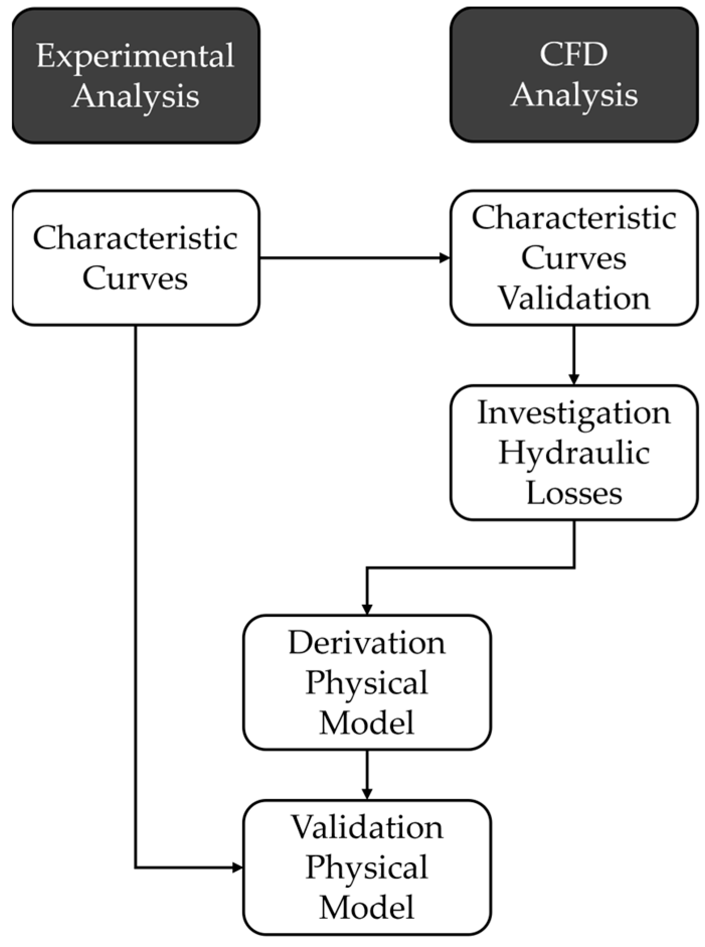
2. Method for Analysing Losses in Centrifugal Pumps with Different Prewhirl Angles

Figure 1 presents a flowchart delineating the discrete phases of the research methodology employed. The investigations are divided into two principal categories: Experimental Analysis and CFD Analysis. During the experimental analysis, the characteristic curves of two radial centrifugal pumps are measured at different prewhirl angles. The database is utilised for two distinct purposes: firstly, to corroborate the findings of the CFD analysis; secondly, to substantiate the physical model that has been determined. This is employed for the purpose of mapping the characteristic curves of the head with varying prewhirl angles.

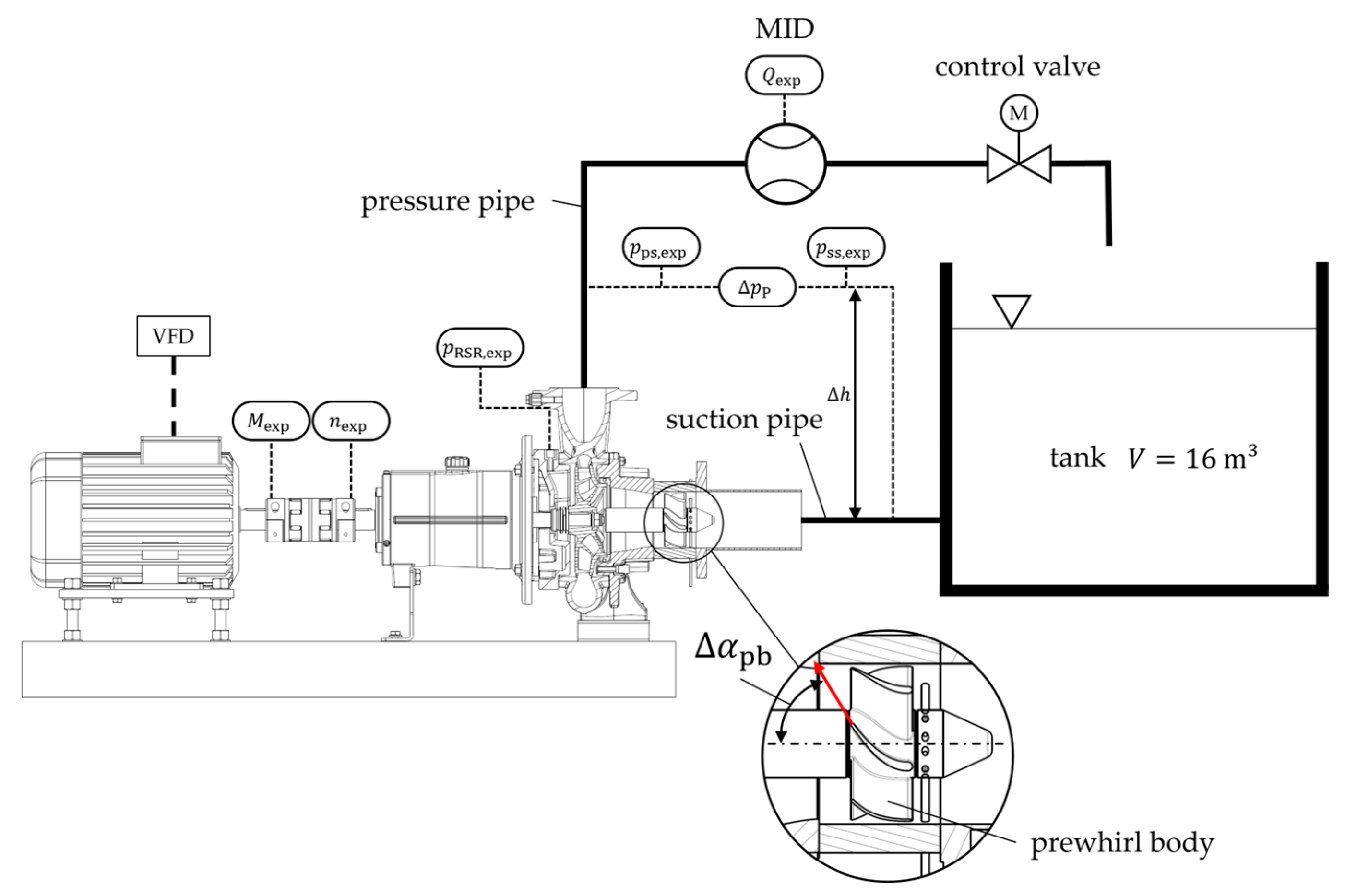
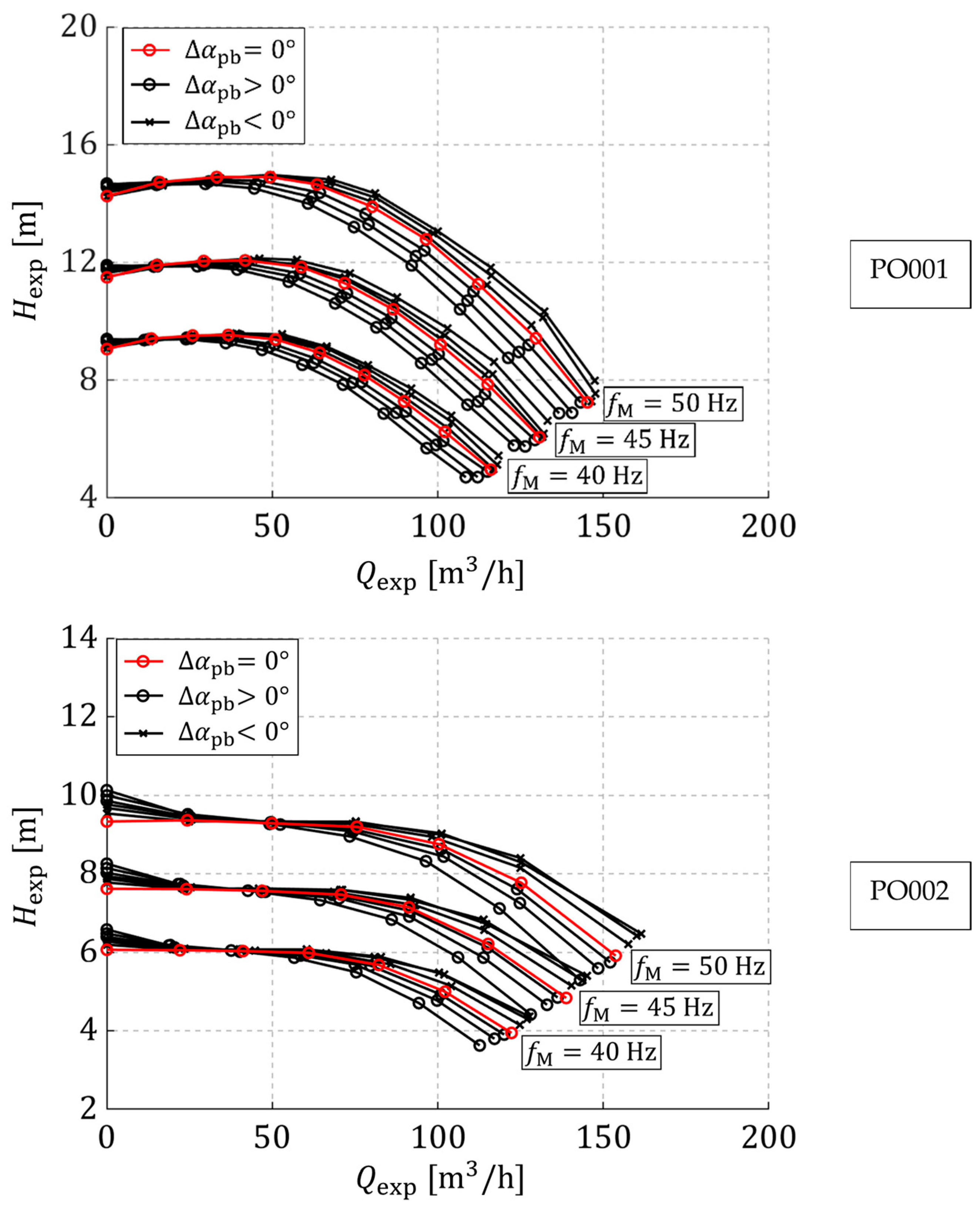
2.1. Experimental Determination of the Head Characteristics with Varying Prewhirl Angles

In order to validate the results of the numerical computer fluid dynamics (CFD) simulations, the head characteristic curves of two pumps were determined experimentally. The two pumps are referred to below as the test object (PO). Important parameters are summarised in

Table 1. Parameters of the two measured pumps (PO001 & PO002). The characteristic curve data in the BEP are indicated by an asterisk (*).

Parameter	PO001	PO002
$\mathrm{specific} \mathrm{speed} \left(n_{\mathrm{q}}\right)$	$36{ \mathrm{m}\mathrm{i}\mathrm{n}}^{-1}$	$54 {\mathrm{m}\mathrm{i}\mathrm{n}}^{-1}$
$\mathrm{outer} \mathrm{diameter} \mathrm{inlet} \left(d_{1\mathrm{a}}\right)$	$124 \mathrm{m}\mathrm{m}$	$122 \mathrm{m}\mathrm{m}$
$\mathrm{inner} \mathrm{diameter} \mathrm{inlet} \left(d_{1\mathrm{i}}\right)$	$46 \mathrm{m}\mathrm{m}$	$47 \mathrm{m}\mathrm{m}$
$\mathrm{diameter} \mathrm{outlet} \left(d_2\right)$	$210 \mathrm{m}\mathrm{m}$	$180 \mathrm{m}\mathrm{m}$
$\mathrm{width} \mathrm{impeller} \mathrm{outlet} \left(b_2\right)$	$22 \mathrm{m}\mathrm{m}$	$33 \mathrm{m}\mathrm{m}$
$\mathrm{number} \mathrm{of} \mathrm{blades} \left(z_{\mathrm{L}}\right)$	$7$	$6$
$\mathrm{blade} \mathrm{angle} \mathrm{outlet} \left({\beta }_{2\mathrm{B}}\right)$	$27°$	$28°$
$\mathrm{mechanical} \mathrm{power} \mathrm{at} n_{\mathrm{N}}$$\left(P_{\mathrm{m}\mathrm{e}\mathrm{c}\mathrm{h}}\right)$	$330 \mathrm{W}$	$70 \mathrm{W}$
$\mathrm{flow} \mathrm{rate} \mathrm{at} \mathrm{BEP} \left(Q^{*}\right)$	$98.6{\displaystyle \frac{{\mathrm{m}}^3}{\mathrm{h}}}$	$113.2{\displaystyle \frac{{\mathrm{m}}^3}{\mathrm{h}}}$
$\mathrm{head} \mathrm{at} \mathrm{BEP} \left(H^{*}\right)$	$13 \mathrm{m}$	$8.2 \mathrm{m}$
$\mathrm{pump} \mathrm{power} \mathrm{at} \mathrm{BEP} \left({P_2}^{*}\right)$	$3143 \mathrm{W}$	$3375 \mathrm{W}$
$\mathrm{nominal} \mathrm{speed} \left(n_{\mathrm{N}}\right)$	$1470 {\mathrm{m}\mathrm{i}\mathrm{n}}^{-1}$	$1470 {\mathrm{m}\mathrm{i}\mathrm{n}}^{-1}$
$\mathrm{performance} \mathrm{factor} \left(\gamma \right)$	$0.81$	$0.78$

. The two pumps exhibit different specific speeds and dimensions. In addition to the geometric parameters, the data for the BEP and the performance factor ($\gamma$) are also given.

The performance factor is defined in accordance with Equation (1) [27]. In Equation (1), $u_2$ represents the circumferential velocity at the impeller outlet, $c_{\mathrm{u}2}$ denotes the circumferential component of the absolute velocity, and $c_{\mathrm{u}2\mathrm{\infty }}$ represents the circumferential component of the absolute velocity in the presence of blade-congruent flow.

$$\gamma =1-{\displaystyle \frac{c_{\mathrm{u}2\mathrm{\infty }}-c_{\mathrm{u}2}}{u_2}}$$

(1)

Figure 2a depicts the velocity triangle within the pump impeller, encompassing all significant velocity components and the definition of the prewhirl angles, with positive and negative signs. The absolute velocity ($c$) can be represented as the sum of its circumferential velocity ($u$) and relative velocity ($w$) or it can be written as the sum of a circumferential component ($c_{\mathrm{u}}$) and a meridional component ($c_{\mathrm{m}}$). The relative velocity describes the flow velocity relative to the rotating pump impeller. The angle $\alpha$ is the angle between $u$ and $c$ and characterises the orientation of the absolute flow with respect to the pump impeller. The flow angle $\beta$ can quantify at flow congruence the blade angle. Figure 2b shows the meridional view of a radial centrifugal pump impeller, highlighting its crucial geometric parameters.

Figure 3 [26] depicts the experimental setup along with the measured variables utilized to assess the characteristic curves at varying prewhirl angles of the prewhirl bodies (${∆\alpha }_{\mathrm{p}\mathrm{b}}$). The prewhirl angle of the flow is a function of the prewhirl bodies. This approach has previously been employed in [26] and is founded upon the proposal by V. Schröder [9]. The prewhirl bodies were manufactured using an additive process and have six blades distributed evenly around the circumference.

In order to determine the head ($H_{\mathrm{e}\mathrm{x}\mathrm{p}}$) experimentally, Equation (2) [26] was employed. The differential pressure (${∆p}_{\mathrm{P}}$) between the static pressure on the pressure side ($p_{\mathrm{p}\mathrm{s},\mathrm{e}\mathrm{x}\mathrm{p}}$) and the suction side ($p_{\mathrm{s}\mathrm{s},\mathrm{e}\mathrm{x}\mathrm{p}}$) is measured by pressure transmitters. The dynamic pressure component is calculated from the flow velocities in the pressure ($v_{\mathrm{p}\mathrm{s}}$) and suction ($v_{\mathrm{s}\mathrm{s}}$) pipe sections at the pressure measurement points. Furthermore, the geodetic height between the suction pipe and the pressure transmitters ($∆h$) is also considered. The head loss of the prewhirl bodies (${∆H}_{\mathrm{p}\mathrm{b}}$) was quantified for each prewhirl body and subsequently incorporated into the head. $g$ denotes the acceleration due to gravity ($g=9.81{\displaystyle \frac{\mathrm{m}}{{\mathrm{s}}^2}}$).

$$H_{\mathrm{e}\mathrm{x}\mathrm{p}}={\displaystyle \frac{{∆p}_{\mathrm{P}}}{g\rho }}+{\displaystyle \frac{v_{\mathrm{p}\mathrm{s}}^2-v_{\mathrm{s}\mathrm{s}}^2}{2g}}+∆h+{∆H}_{\mathrm{p}\mathrm{b}}$$

(2)

In addition to the pressures $p_{\mathrm{p}\mathrm{s},\mathrm{e}\mathrm{x}\mathrm{p}}$ and $p_{\mathrm{s}\mathrm{s},\mathrm{e}\mathrm{x}\mathrm{p}}$, a measured pressure value was also recorded in the impeller side gap between the pump impeller back disc and the pump housing ($p_{\mathrm{R}\mathrm{S}\mathrm{R},\mathrm{e}\mathrm{x}\mathrm{p}}$). To determine the power consumption of the pump, it is necessary to measure the torque ($M_{\mathrm{e}\mathrm{x}\mathrm{p}}$) and the speed ($n_{\mathrm{e}\mathrm{x}\mathrm{p}}$) via a torque-measuring shaft. The speed of the pump can be adjusted by means of a frequency converter (VFD). The pump power consumption ($P_{2,\mathrm{e}\mathrm{x}\mathrm{p}}$) is calculated according to Equation (3). The power consumption of the pump includes the mechanical power loss of the bearing and the mechanical seal, which is designated as $P_{\mathrm{m}\mathrm{e}\mathrm{c}\mathrm{h}}$. This was specified in Table 1 and determined experimentally.

$$P_{2,\mathrm{e}\mathrm{x}\mathrm{p}}={2\pi M}_{\mathrm{e}\mathrm{x}\mathrm{p}}{n}_{\mathrm{e}\mathrm{x}\mathrm{p}}$$

(3)

The flow rate ($Q_{\mathrm{e}\mathrm{x}\mathrm{p}}$) can be adjusted by a control valve in the pressure pipe through the process of throttling and is then measured by a magnetic inductive flow meter (MID). The pumped liquid is taken from a tank with a volume of $V=16 {\mathrm{m}}^3$ and returned by the pump. Given the considerable volume of the tank and the brief measurement period, it may be reasonably assumed that the pumped medium will not experience a significant degree of heating. Consequently, the density of the pumped medium was assumed to be constant at $\rho =998{\displaystyle \frac{\mathrm{k}\mathrm{g}}{{\mathrm{m}}^3}}$. For each measured operating point, all values were sampled at a sampling rate of $f_{\mathrm{S}}=500 \mathrm{H}\mathrm{z}$ over a measurement period of $t_{\mathrm{S}}=10 \mathrm{s}$. Subsequently, the mean values were calculated for the operating points. The maximum relative errors of the individual measured variables and the calculated variables can be found in Appendix A. The maximum relative errors of the calculated variables were determined using Gauss’s law of error propagation.

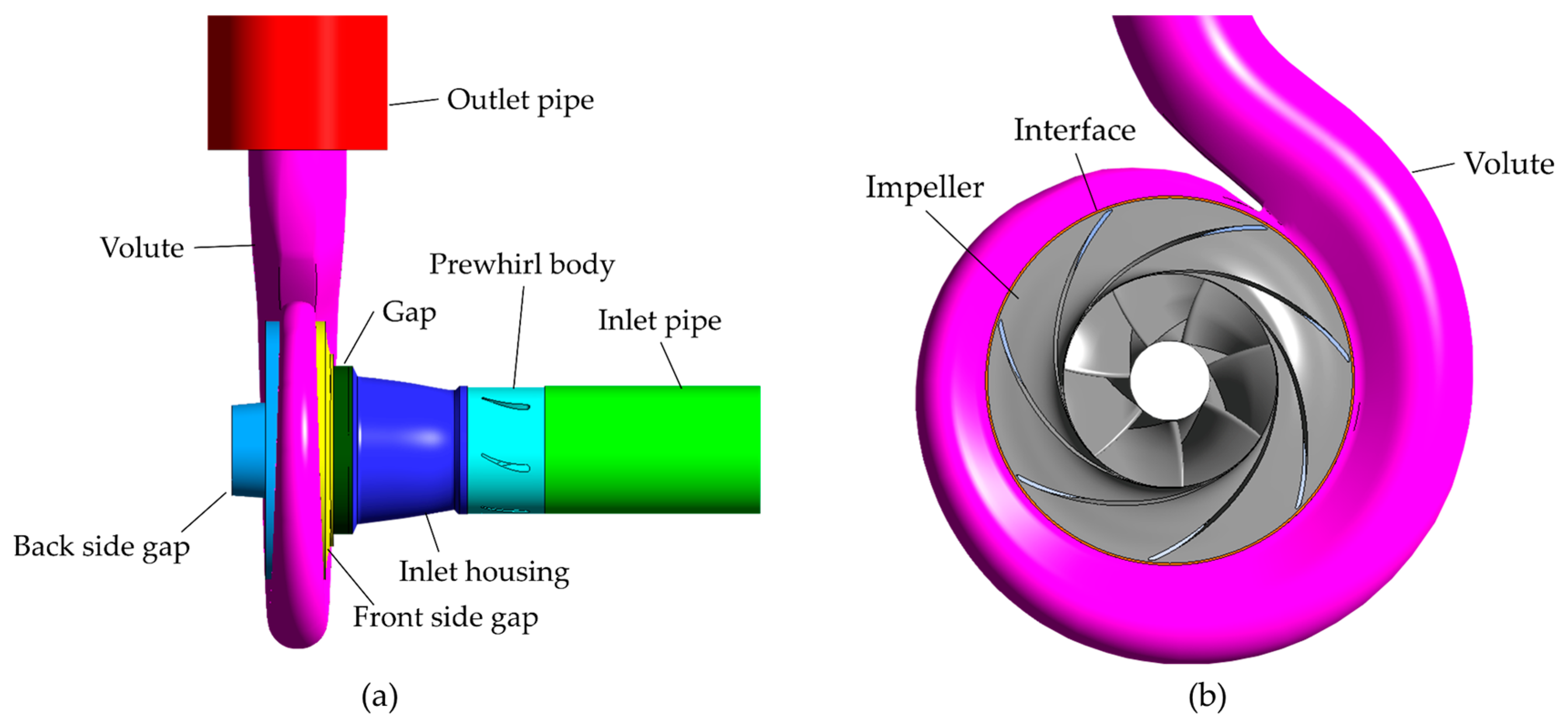
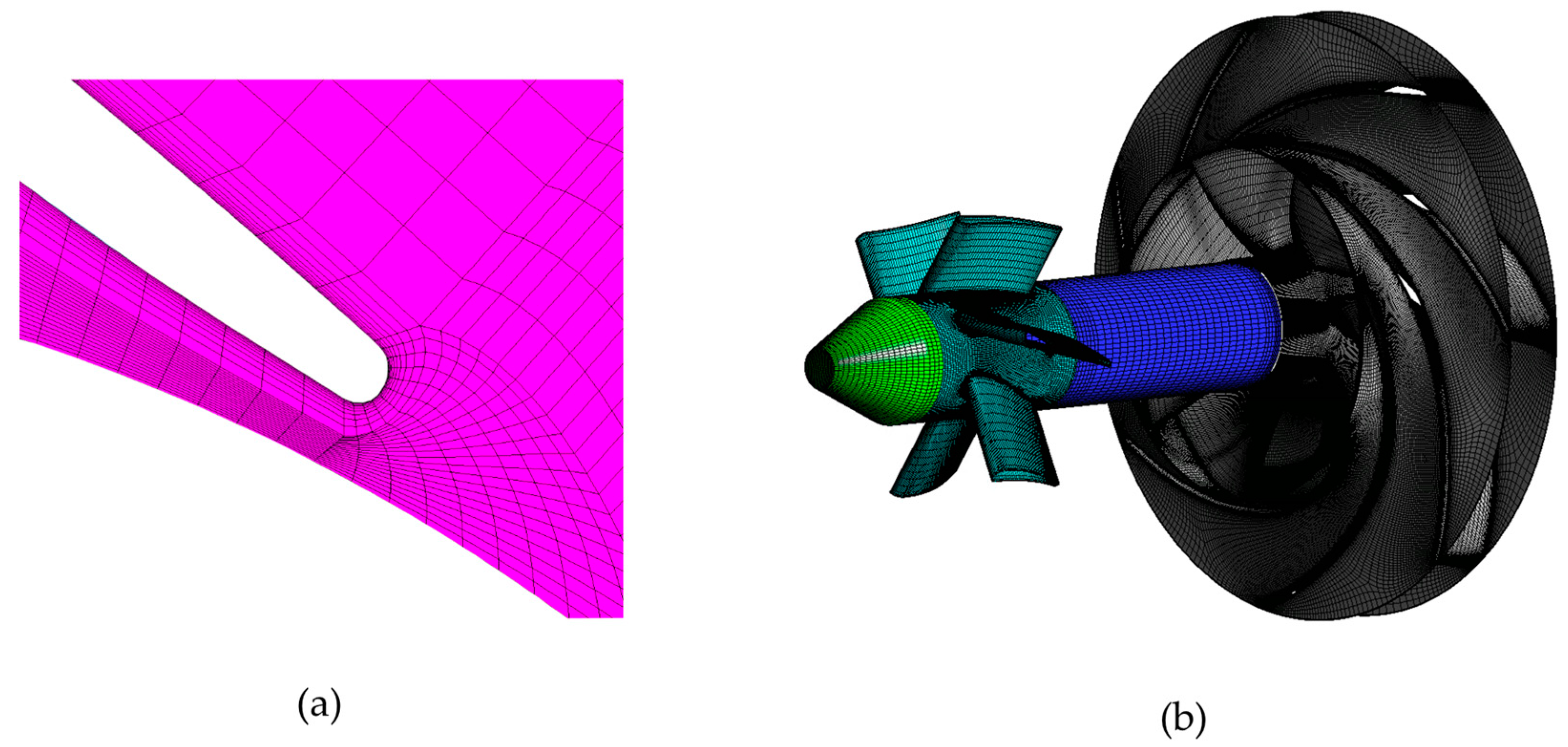
2.2. 3D Model and Meshes for the Numerical Investigation of Hydraulic Losses

The CFD simulation for the analysis of hydraulic losses is based on a three-dimensional mesh of the pump flow area. For PO001, three-dimensional geometries were generated for three prewhirl bodies with prewhirl angles ${∆\alpha }_{\mathrm{p}\mathrm{b}}\in \left\{-30°;0°;+30°\right\}$. Figure 4a depicts the side view, which includes all externally visible flow areas. The inlet pipe has a length that is six times the hydraulic diameter, which allows for the exclusion of influences of the boundary conditions. The flow area of the prewhirl body is behind the inlet pipe. The prewhirl body flow domain contains the six blades of the prewhirl bodies, which were employed in the experimental measurements. The inlet housing, which is connected to the gap as well as the impeller, follows the flow area of the prewhirl body. The front and back side gaps are formed between the discs of the impeller and the housing, each of which is represented by a flow area. Figure 4a illustrates the abrupt widening of the cross-section that occurs at the transition between the volute and the outlet pipe. This transition is in accordance with the measurement setup.

Figure 4b depicts the three-dimensional geometries of the flow area in front view, omitting the inlet pipe, side gaps, gap and outlet pipe with volute, interface and impeller. The flow area of the interface is situated between the flow areas of the impeller and the volute. The interface connects the main flow from the impeller to the volute, with the front and back side gap. As illustrated, the flow area of PO001 was completely mapped. In some of the works discussed in the introduction, the mapping was limited to the flow areas of the inlet and outlet pipes, the volute and the impeller. This results in differences between the simulation and the experimental measurement data. Furthermore, the losses in the impeller side gaps cannot be analysed. Furthermore, the gap flow from the impeller outlet via the front side gap and the gap into the inlet housing, along with the associated losses, are not taken into account.

The three-dimensional geometries illustrated in Figure 4 were individually meshed. The impeller was meshed using TurboGrid 2022 R1. The meshing was implemented for a passage situated between two blades and was subsequently replicated for all blades positioned around the pump’s axis of rotation. The flow domains of the prewhirl bodies were also meshed using this method. The remaining flow domains were meshed using the SpaceClaim 2022 R1 meshing tool. The near wall layers were refined in a uniform manner for all geometries. The height of the final wall node layer was found to be $∆y=0.05 \mathrm{m}\mathrm{m}$.

P. Limbach et al. demonstrated that the flow patterns of centrifugal pumps can be accurately replicated with meshes comprising a lower number of nodes [28]. A comparison was conducted between three meshes comprising between 1.8 million and 16 million nodes. It was demonstrated that even at a node count of 1.8 million, it was possible to achieve small deviations between the simulation and the experiment [28]. P. Lin et al. demonstrated that node numbers between 1.2 million and 4.1 million nodes exert only a minor influence on the results [19]. A mesh sensitivity study was conducted to demonstrate the independence of the results from the meshes. In order to achieve this objective, four meshes with varying node numbers were constructed. The flow area with ${∆\alpha }_{\mathrm{p}\mathrm{b}}=0°$ was meshed. The configuration of the simulations is detailed in the subsequent chapter.

Table 2. The results of the mesh sensitivity analysis are presented together with an indication of the number of nodes, the results of head and power consumption.

	Mesh 1	Mesh 2	Mesh 3	Mesh 4
Node Number	1,339,728	2,001,547	2,376,901	4,883,055
$H$	$12.70 \mathrm{m}$	$12.78 \mathrm{m}$	$12.77 \mathrm{m}$	$12.79 \mathrm{m}$
$P_2$	$4.422 \mathrm{k}\mathrm{W}$	$4.438 \mathrm{k}\mathrm{W}$	$4.436 \mathrm{k}\mathrm{W}$	$4.437 \mathrm{k}\mathrm{W}$

presents the findings of the mesh sensitivity analysis. The meshes are designated as Mesh 1 to Mesh 4, respectively. Table 2 presents a summary of the number of nodes, the simulated head ($H$) and power consumption ($P_2$). In accordance with the findings of P. Limbach et al. [28] and P. Lin et al. [19], the outcomes pertaining to node numbers within the range of 1 to 5 Mio. are not contingent upon the underlying meshes. Only minor fluctuations can be observed. The results are therefore independent of the mesh.

We use mesh nodes numbers of 2.3 to 2.8 Mio. mesh nodes (see

Table 3. The number of nodes in the meshes for the three investigated prewhirl body angles ${∆\alpha }_{\mathrm{p}\mathrm{b}}\in \left\{-30°;0°;+30°\right\}$.

${\mathbf{∆}\mathit{\alpha }}_{\mathbf{p}\mathbf{b}}\mathbf{=}\mathbf{-}\mathbf{30}\mathbf{°}$	${\mathbf{∆}\mathit{\alpha }}_{\mathbf{p}\mathbf{b}}\mathbf{=}\mathbf{0}\mathbf{°}$	${\mathbf{∆}\mathit{\alpha }}_{\mathbf{p}\mathbf{b}}\mathbf{=}\mathbf{+}\mathbf{30}\mathbf{°}$
2,744,701	2,376,901	2,848,057

), i.e., according to the works cited and mesh sensitivity analysis above, sufficiently large to be reliable. The meshes are block structured and are hexagonal in shape. Table 3 presents the number of nodes for the meshes of the three investigated prewhirl body angles, ${∆\alpha }_{\mathrm{p}\mathrm{b}}\in \left\{-30°;0°;+30°\right\}$.

In addition to the number of nodes, the nature of the meshes at exposed points is important. These are all those points where potential flow separation and significant fluid-structure interactions may occur. For this reason, the meshes at critical points are presented in greater detail in Figure 5. Figure 5a illustrates the nature of the mesh around the tongue of the volute. At this juncture, the flow bifurcates, with one branch returning to the volute and the other continuing to the discharge. The block structure of the meshes allows for the contour of the tongue to be modelled using hexagonal elements. Furthermore, the dissolution of the near wall layers can be identified. Figure 5b depicts the mesh on the surface of the impeller and the prewhirl body. The advantages of block structuring for mapping the twisted blade geometry are also evident in this case. The blades of the prewhirl bodies are also depicted with a block structured mesh. The diameter of the impeller hub has been drawn up to the prewhirl bodies, which is consistent with the experimental setup. It is important to note that the prewhirl bodies do not rotate at the same speed as the impeller. Rather, they remain fixed within the flow. Furthermore, it can be observed that the hub of the prewhirl bodies extends from the inlet pipe via the inlet housing to the hub of the impeller.

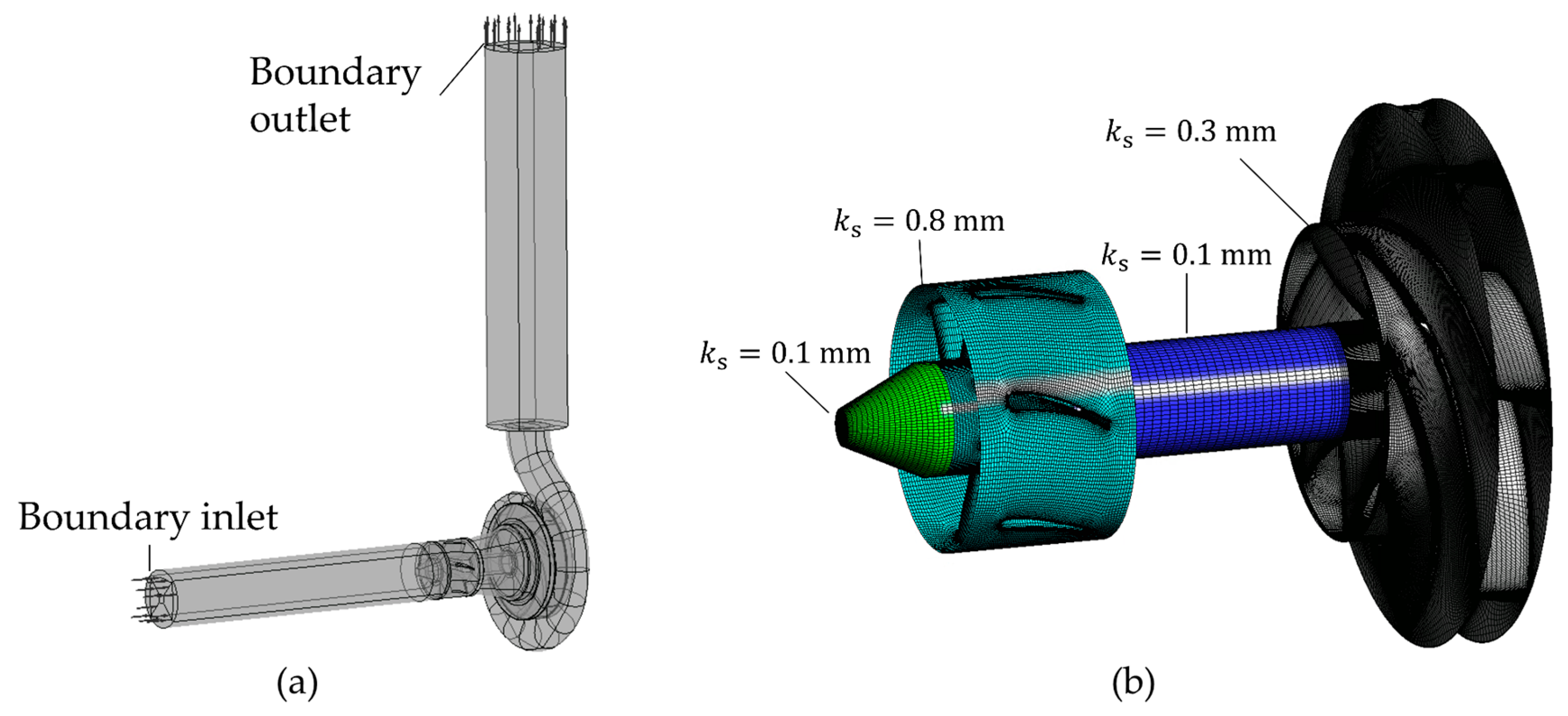
2.3. Setup of the CFD Simulation

The CFD simulation was conducted using ANSYS-CFX 2022 R1 software, employing the finite volume method for discretization [29]. The simulation was performed as an Unsteady-Reynolds-Averaged-Navier-Stokes (URANS) [29] simulation. A stationary simulation was conducted for each operating point to initialize the simulation. Five operating points with varying flow rates of $Q\in \left\{60{\displaystyle \frac{{\mathrm{m}}^3}{\mathrm{h}}}; 80{\displaystyle \frac{{\mathrm{m}}^3}{\mathrm{h}}};100{\displaystyle \frac{{\mathrm{m}}^3}{\mathrm{h}}};120{\displaystyle \frac{{\mathrm{m}}^3}{\mathrm{h}}};140{\displaystyle \frac{{\mathrm{m}}^3}{\mathrm{h}}}\right\}$ were simulated for all three prewhirl body angles. Figure 6a depicts the entire flow area for the simulation. The boundary conditions at the inlet of the flow area (boundary inlet) and at the outlet of the flow area (boundary outlet) are indicated by arrows. A static pressure of $p=0 \mathrm{P}\mathrm{a}$ and a medium turbulence intensity of $5\%$ were considered for the boundary condition at the inlet. A constant mass flow ($\dot{m}$) normal to the surface was specified as the boundary condition at the outlet. The mass flow was calculated in accordance with Equation (4).

$$\dot{m}=\rho Q$$

(4)

It was assumed that the solid walls were smooth. The conditions do not apply to the surfaces depicted in Figure 6b. The equivalent sand grain roughnesses ($k_{\mathrm{s}}$) were considered for these surfaces. These factors exert a non-negligible influence on the head, as demonstrated by P. Limbach et al. [28]. The surface of the prewhirl bodies is printed in layers, which results in a higher equivalent sand grain roughness compared to the other surfaces. The pump impeller, which is constructed from cast aluminium multi-material bronze (CuAl), also exhibits a higher degree of sand grain roughness. In addition to the surfaces depicted in Figure 6b, equivalent sand roughnesses with a value of $k_{\mathrm{s}}=0.3 \mathrm{m}\mathrm{m}$ were also considered for the walls of the pump impeller in the impeller side gaps and the gap.

A constant speed of $n=1470 {\mathrm{m}\mathrm{i}\mathrm{n}}^{-1}$ was assumed for the flow area in the impeller, as well as for the walls of the impeller in the impeller side gaps and in the gap. The impeller is discretised with an angle of $∆\phi ≔3°$ for each revolution. Four revolutions of the pump impeller were calculated on the basis of the initialising steady-state simulations. This yields a total of 480 time steps, calculated with a maximum iteration number of 10 iterations. An effective residual of 5 × 10⁵ and a conversation target of $1\%$ were assumed as convergence criteria. The shear stress transport (SST) [29] model, as proposed by F. Menter in [30], was employed to map the turbulence.

3. Analysis and Discussion of the Results

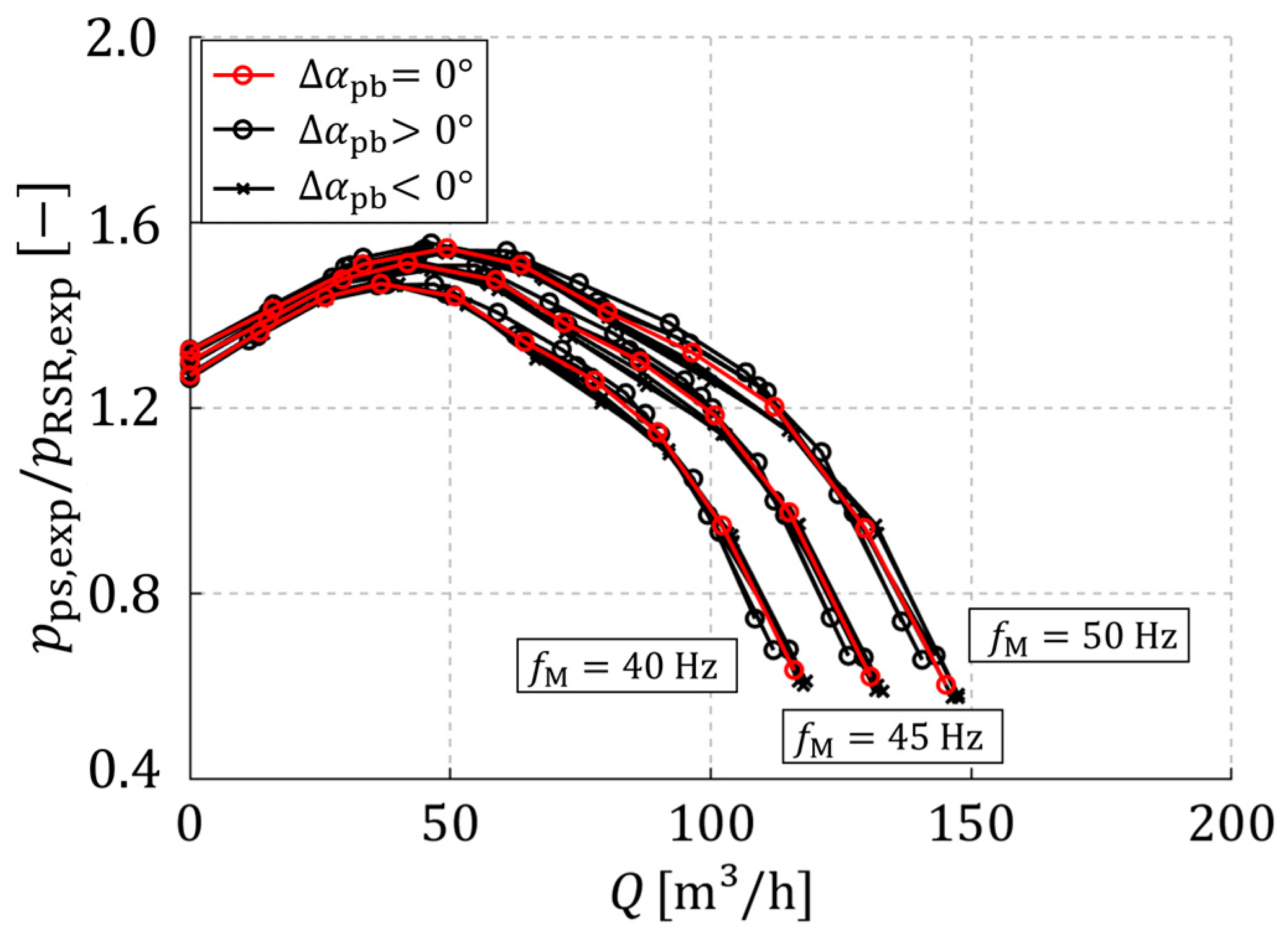
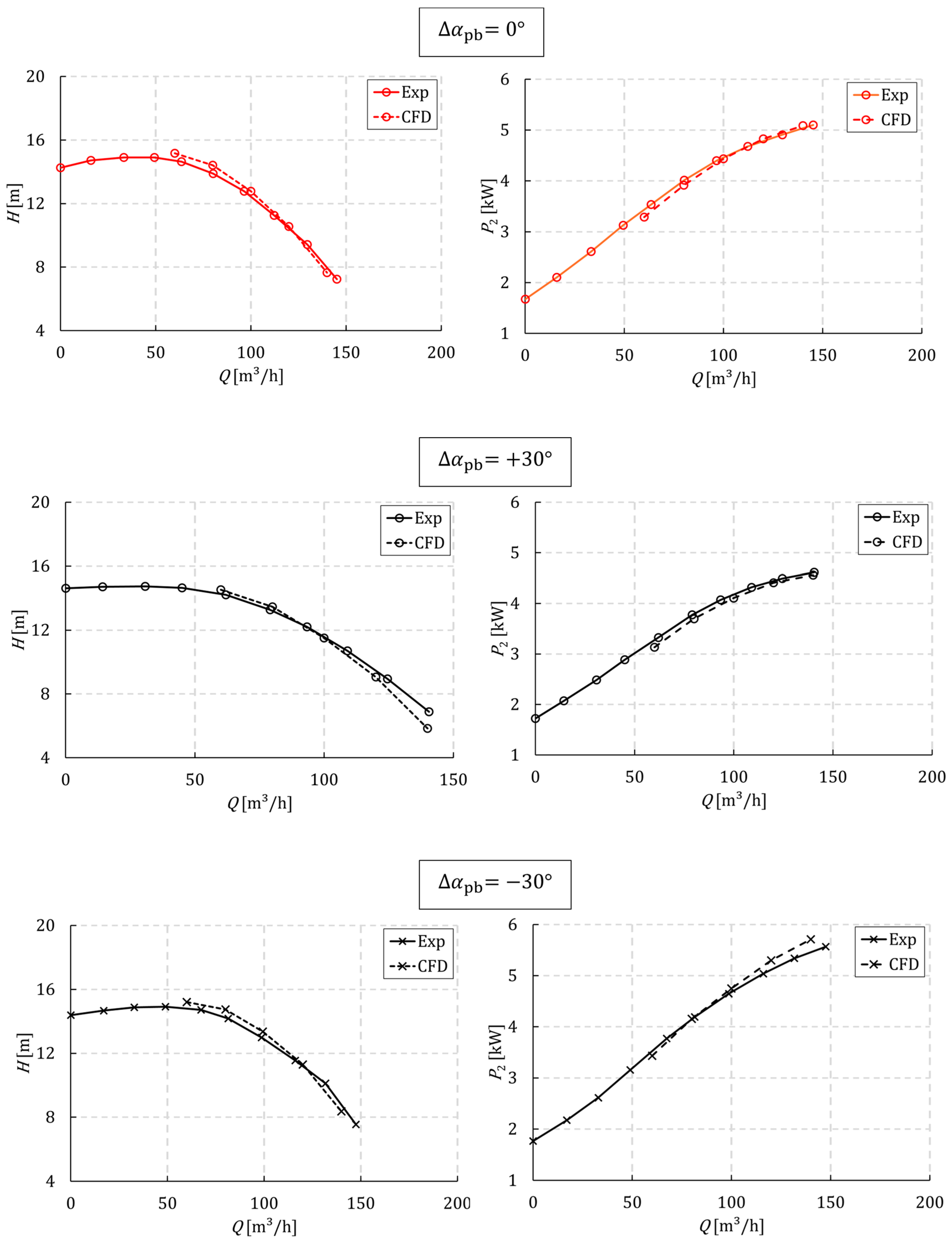
3.1. Analysis and Discussion of the Experimental Results

Figure 7 illustrates the characteristic curves of the head plotted against the flow rate for PO001 (figure above) and PO002 (figure below). The circles (${∆\alpha }_{\mathrm{p}\mathrm{b}}=0°$ and ${∆\alpha }_{\mathrm{p}\mathrm{b}}>0°$) and crosses (${∆\alpha }_{pb}<0°$) represent the measured data points, which were connected linearly. The characteristic curves for the prewhirl body with ${∆\alpha }_{\mathrm{p}\mathrm{b}}=0°$ are depicted in red, while all characteristic curves measured with ${∆\alpha }_{\mathrm{p}\mathrm{b}}>0°$ and ${∆\alpha }_{\mathrm{p}\mathrm{b}}<0°$ are shown in black. The characteristic curves are arranged in accordance with the motor frequencies ($f_{\mathrm{M}}$) indicated on the VFD. As the measured speed ($n_{\mathrm{e}\mathrm{x}\mathrm{p}}$) is dependent on the power consumption, the value of $f_{\mathrm{M}}$ was specified. The characteristic curves of the heads are demonstrably influenced by the prewhirl body angle. As illustrated in Figure 2b, the circumferential components of the absolute velocity at the impeller inlet ($c_{\mathrm{u}1}$) are subject to influence from the prewhirl angle. It can be demonstrated that positive prewhirl angles (${∆\alpha }_1$) result in a reduction of the Euler equation of turbomachines, as shown in Equation (5) [27]. Conversely, when negative prewhirl angles are present, an increase in the specific impeller work ($\tilde{Y}$) is observed. The velocity components $u_{1,\mathrm{m}}$ and $c_{\mathrm{u}1,\mathrm{m}}$ are defined as the velocity components on the mean meridian streamline of the impeller.

$$\tilde{Y}=u_2{c}_{\mathrm{u}2}-u_{1,\mathrm{m}}{c}_{\mathrm{u}1,\mathrm{m}}$$

(5)

$$H=\tilde{Y}{\eta }_{\mathrm{h}}$$

(6)

The head of the pump is adjusted according to Equation (6) [27]. In Equation (6), ${\eta }_{\mathrm{h}}$ represents the hydraulic efficiency of the pump which includes all hydraulic losses in the pump. It can be observed that while the head decreases continuously with positive prewhirl angles (${∆\alpha }_{\mathrm{p}\mathrm{b}}>0°$), the increase in head appears to reach a plateau with increasing negative prewhirl angles (${∆\alpha }_{\mathrm{p}\mathrm{b}}<0°$). This phenomenon is more pronounced in the case of PO002 than in the case of PO001. As indicated by Equation (6), this suggests a variable hydraulic efficiency. This phenomenon can be attributed to the occurrence of varying flow losses within the pump.

A further investigation of the hydraulic losses in the pump can be conducted by analysing the pressure in the impeller back side gap ($p_{\mathrm{R}\mathrm{S}\mathrm{R},\mathrm{e}\mathrm{x}\mathrm{p}}$). Figure 8 illustrates the ratio of the static pressure difference between the static pressure at the pressure side ($p_{\mathrm{p}\mathrm{s},\mathrm{e}\mathrm{x}\mathrm{p}}$) and the static pressure in the back side gap ($p_{\mathrm{R}\mathrm{S}\mathrm{R},\mathrm{e}\mathrm{x}\mathrm{p}}$) for PO001 at varying motor frequencies ($f_{\mathrm{M}}$). The representation of the characteristic curves is consistent with the depiction in Figure 7. At all motor frequencies, the pressure ratio between the individual characteristic curves exhibits only slight deviations when varying ${∆\alpha }_{\mathrm{p}\mathrm{b}}$.

The back side gap is directly coupled to the impeller outlet. The pressure in the back side gap can be calculated using Equation (7) [27]. $c_{\mathrm{p},\mathrm{R}\mathrm{S}\mathrm{R}}$ denotes the pressure reduction coefficient [27], which quantifies the pressure loss between the pressure at the impeller outlet ($p_2$) and $p_{\mathrm{R}\mathrm{S}\mathrm{R}}$. The value of $p_{\mathrm{R}\mathrm{S}\mathrm{R}}$ therefore depends on $p_2$, $u_2$ and $c_{\mathrm{p},\mathrm{R}\mathrm{S}\mathrm{R}}$. It can be demonstrated that variations in $p_{\mathrm{R}\mathrm{S}\mathrm{R}}$ are attributable to $p_2$ at a constant speed and geometry.

$$p_{\mathrm{R}\mathrm{S}\mathrm{R}}=p_2-{\displaystyle \frac{\rho }{2}}{u}_2^2{c}_{\mathrm{p},\mathrm{R}\mathrm{S}\mathrm{R}}.$$

(7)

The pressure ratio can be expressed as follows:

$${\displaystyle \frac{p_{\mathrm{P}\mathrm{S}}}{p_{\mathrm{R}\mathrm{S}\mathrm{R}}}}={\displaystyle \frac{p_2+{∆p}_{\mathrm{G}\mathrm{L}}-{∆p}_{\mathrm{G}\mathrm{L},\mathrm{l}\mathrm{o}\mathrm{s}\mathrm{s}}}{p_2-\frac{\rho }{2}{u}_2^2{c}_{\mathrm{p},\mathrm{R}\mathrm{S}\mathrm{R}}}},$$

(8)

The variable ${∆p}_{\mathrm{G}\mathrm{L}}$ denotes the pressure increase in the volute, while ${∆p}_{\mathrm{G}\mathrm{L},\mathrm{l}\mathrm{o}\mathrm{s}\mathrm{s}}$ represents the volute’s pressure loss. It can be assumed that the proportionality approach $p_2\propto H\propto n^2$ applies to the pressure at the impeller outlet [27]. Equation (7) illustrates that $∆p_{\mathrm{R}\mathrm{S}\mathrm{R}}\propto u_2^2\propto n^2$ applies to the pressure drop between the impeller outlet and the measuring point in the back side gap (${∆p}_{\mathrm{R}\mathrm{S}\mathrm{R}}$). It can be assumed that for the increase in pressure at the volute and pressure loss of the volute, ${∆p}_{\mathrm{G}\mathrm{L}}, {∆p}_{\mathrm{G}\mathrm{L},\mathrm{l}\mathrm{o}\mathrm{s}\mathrm{s}}\propto Q^2$ [27]. This shows that ${∆p}_{\mathrm{G}\mathrm{L}}$ and ${∆p}_{\mathrm{G}\mathrm{L},\mathrm{l}\mathrm{o}\mathrm{s}\mathrm{s}}$ do not vary when the speed is varied. The increase in flow losses and the associated reduction in hydraulic efficiency can be attributed to the impeller.

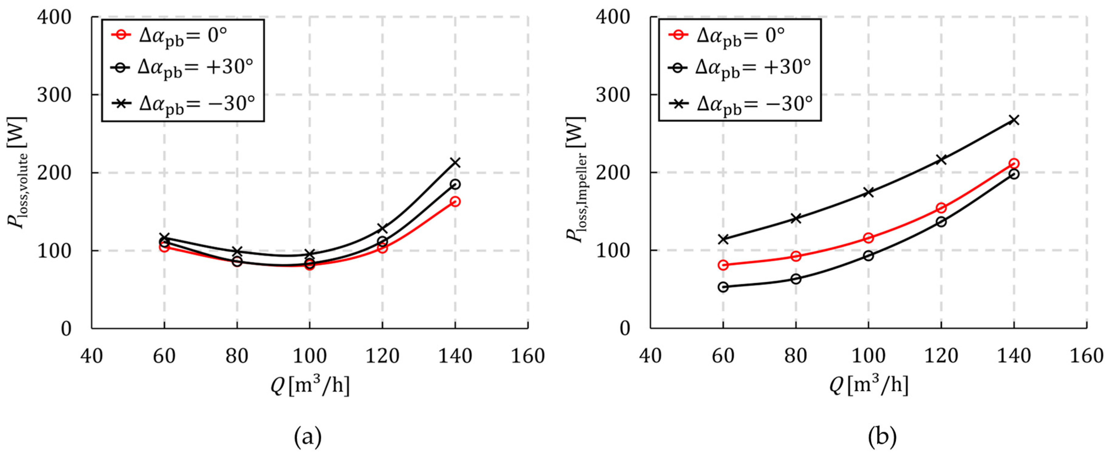
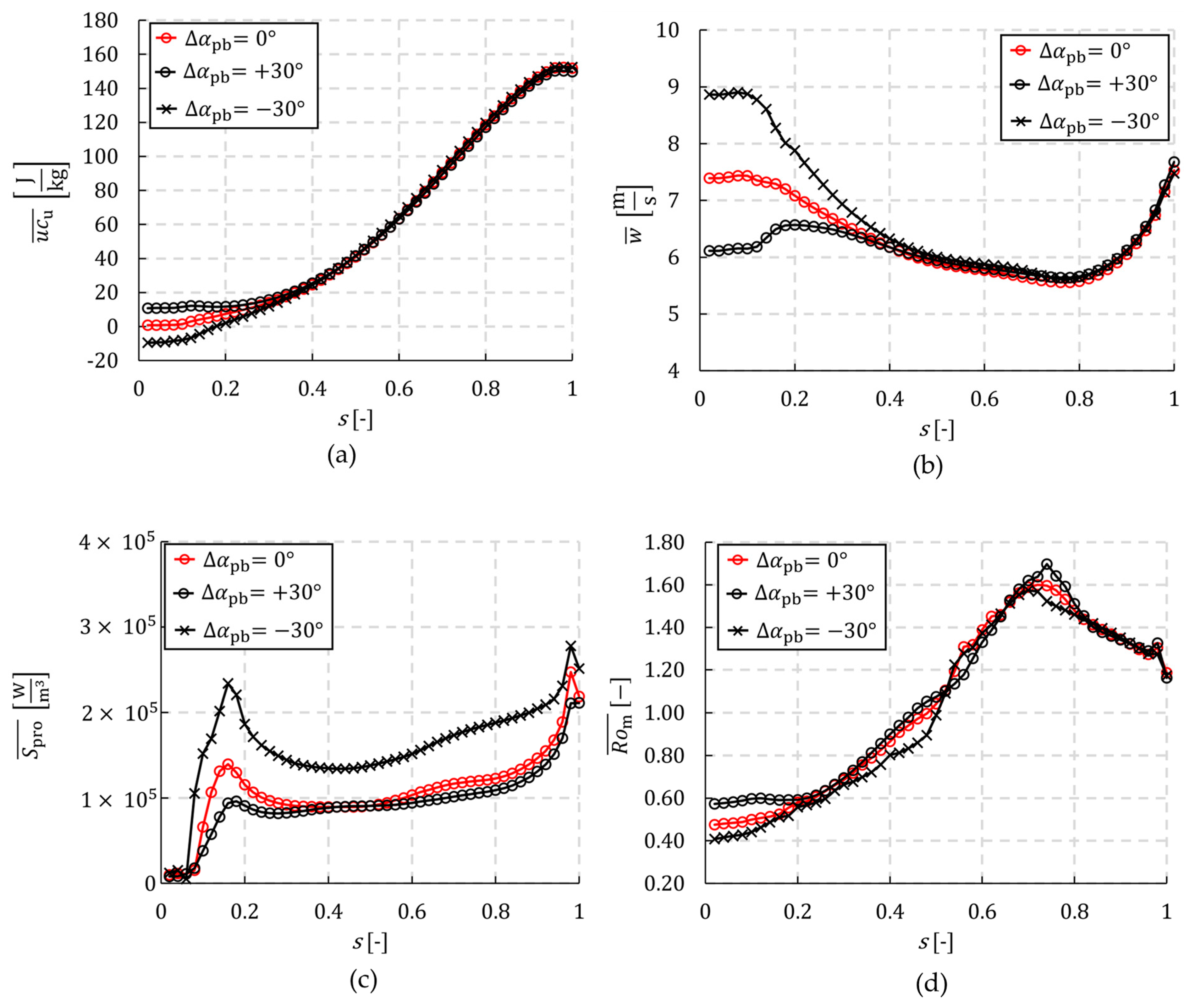
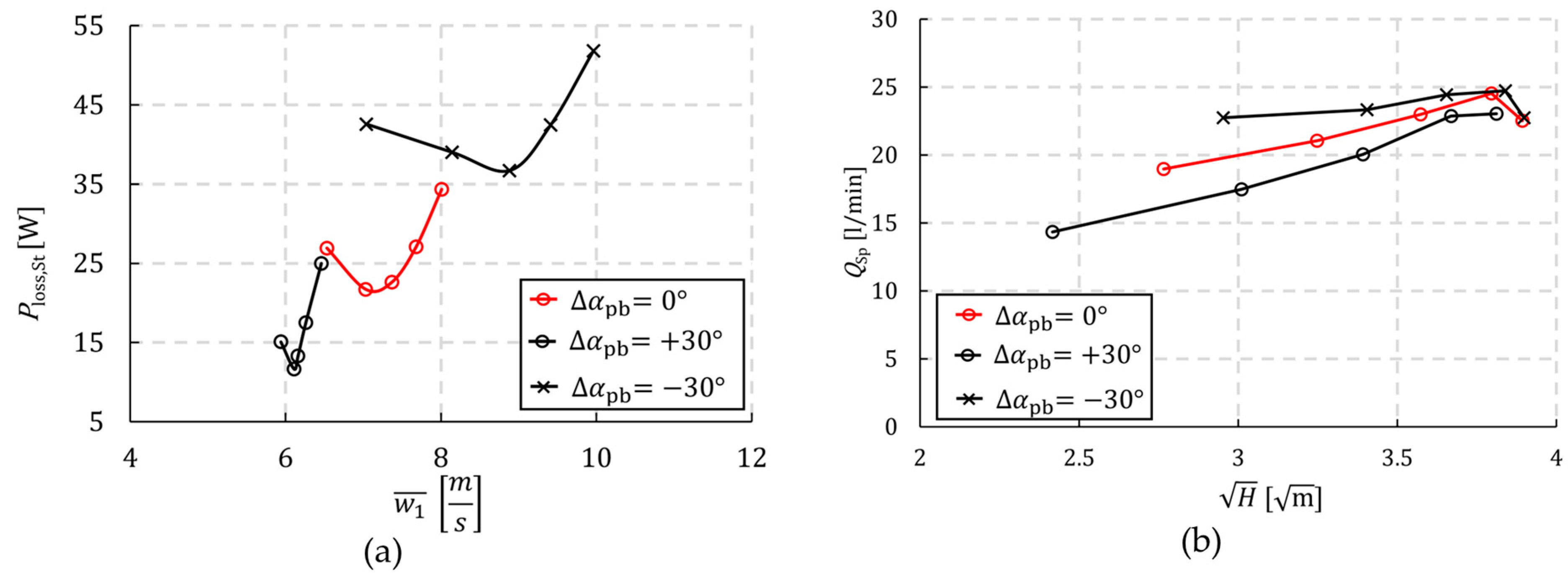
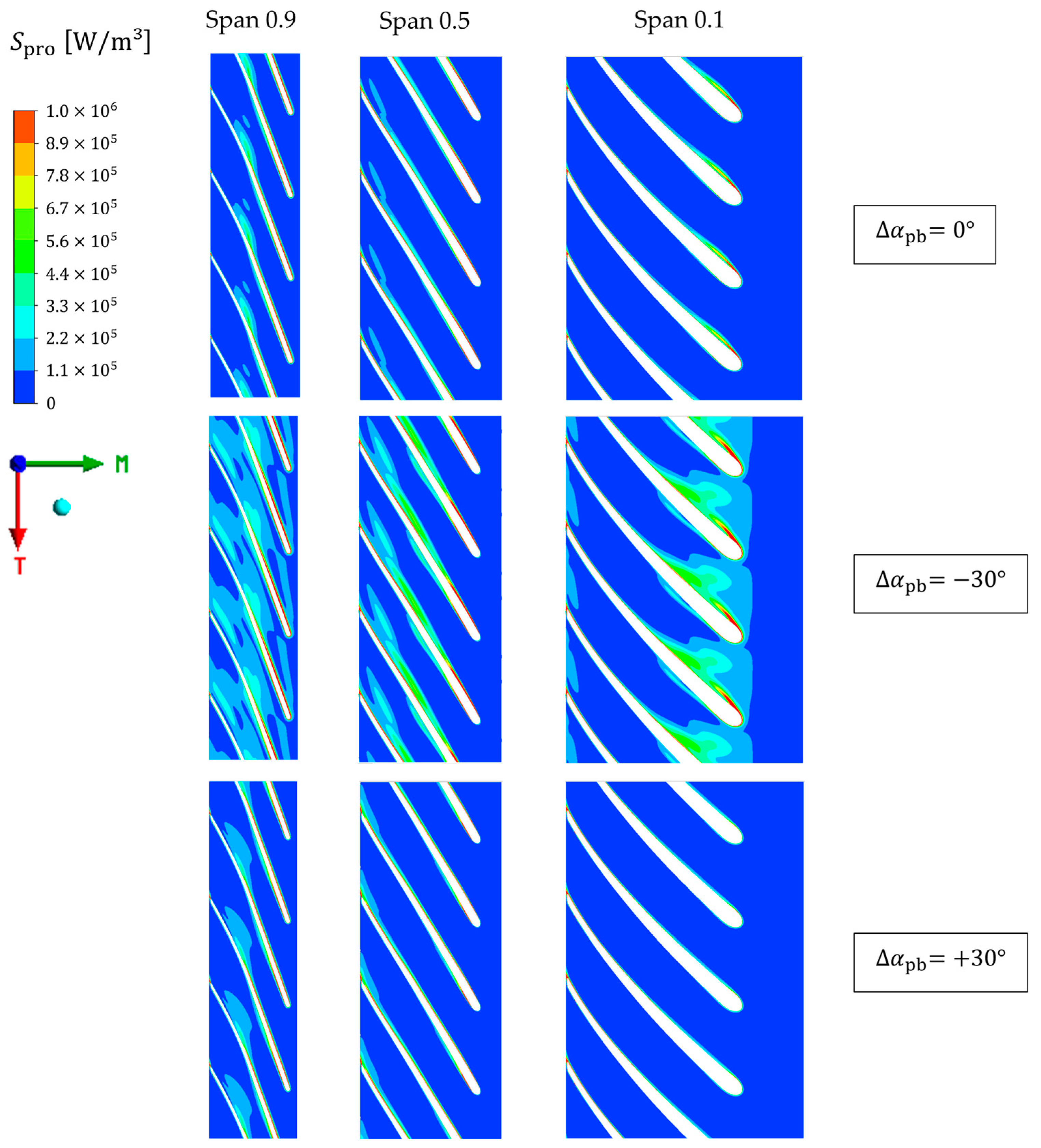
3.2. Validation of the CFD Simulation and Analysis of the Loss Behaviour

The head determined by the CFD simulation (CFD) is illustrated in Figure 9, accompanied by the corresponding measurements (Exp). The left-hand side diagrams depict the head, while the right-hand side diagrams illustrate the power consumption for the three prewhirl body angles under analysis. The head was identified as being located at the boundary outlet, as well as between the prewhirl body and inlet housing. For ${∆\alpha }_{\mathrm{p}\mathrm{b}}=0°$, there are slight deviations for flow rates $Q<100{\displaystyle \frac{{\mathrm{m}}^3}{\mathrm{h}}}$. Furthermore, deviations are observable in the remaining prewhirl body angles. For ${∆\alpha }_{\mathrm{p}\mathrm{b}}=+30°$, larger deviations occur at $Q>120{\displaystyle \frac{{\mathrm{m}}^3}{\mathrm{h}}}$. The maximum relative deviation between the simulation and the measurements is less than 4%. Only the operating point at $Q=140{\displaystyle \frac{{\mathrm{m}}^3}{\mathrm{h}}}$ of ${∆\alpha }_{\mathrm{p}\mathrm{b}}=+30°$ is an exception and exhibits a deviation greater than $10\%$. In conclusion, the observed deviations are significantly below those reported by Lin et al. [19], rendering them suitable for the analysis of the flow fields and losses. Figure 9 also shows the characteristic curves of the power consumption ($P_2$) for the measurements (Exp) and the simulations (CFD) with variation of the prewhirl body angle ${∆\alpha }_{\mathrm{p}\mathrm{b}}\in \left\{-30°;0°;+30°\right\}$. It is important to note that the power consumption in the measurements is larger than that in the simulation due to mechanical losses ($P_{\mathrm{m}\mathrm{e}\mathrm{c}\mathrm{h}}$). Nevertheless, there is a high degree of concordance between experimental and simulated results. In particular, the simulation is expected to accurately model secondary losses, such as friction in the impeller side gaps.

As previously outlined in the introduction, the entropy production method is commonly employed to examine the causes of losses in centrifugal pumps. According to the URANS, the entropy production ($S_{\mathrm{p}\mathrm{r}\mathrm{o}}$) is decomposed into an averaged (${\overline{S}}_{\mathrm{p}\mathrm{r}\mathrm{o}}$) and a turbulent ($S_{\mathrm{p}\mathrm{r}\mathrm{o}}$′) part, as shown in Equation (9) [22,31]. Equation (10) [22,31] illustrates the averaged entropy production, whereas Equation (11) [22,31] depicts the turbulent entropy production. The equations of [22,31] were multiplied by the temperature.

$$S_{\mathrm{p}\mathrm{r}\mathrm{o}}={\overline{S}}_{\mathrm{p}\mathrm{r}\mathrm{o}}+{S_{\mathrm{p}\mathrm{r}\mathrm{o}}}^{\prime }$$

(9)

$${\overline{S}}_{\mathrm{p}\mathrm{r}\mathrm{o}}=\mu \left(2\left({\left({\displaystyle \frac{\partial \overline{u}}{\partial x}}\right)}^2+{\left({\displaystyle \frac{\partial \overline{v}}{\partial y}}\right)}^2+{\left({\displaystyle \frac{\partial \overline{w}}{\partial z}}\right)}^2\right)+{\left({\displaystyle \frac{\partial \overline{u}}{\partial y}}+{\displaystyle \frac{\partial \overline{v}}{\partial x}}\right)}^2+{\left({\displaystyle \frac{\partial \overline{u}}{\partial z}}+{\displaystyle \frac{\partial \overline{w}}{\partial x}}\right)}^2+{\left({\displaystyle \frac{\partial \overline{v}}{\partial z}}+{\displaystyle \frac{\partial \overline{w}}{\partial y}}\right)}^2\right)$$

(10)

$$S_{\mathrm{p}\mathrm{r}\mathrm{o}}^{\prime }=\mu \left(2\left({\left({\displaystyle \frac{\partial u^{\prime }}{\partial x}}\right)}^2+{\left({\displaystyle \frac{\partial v^{\prime }}{\partial y}}\right)}^2+{\left({\displaystyle \frac{\partial w^{\prime }}{\partial z}}\right)}^2\right)+{\left({\displaystyle \frac{\partial u^{\prime }}{\partial y}}+{\displaystyle \frac{\partial v^{\prime }}{\partial x}}\right)}^2+{\left({\displaystyle \frac{\partial u^{\prime }}{\partial z}}+{\displaystyle \frac{\partial w^{\prime }}{\partial x}}\right)}^2+{\left({\displaystyle \frac{\partial v^{\prime }}{\partial z}}+{\displaystyle \frac{\partial w^{\prime }}{\partial y}}\right)}^2\right)$$

(11)

The velocity components in the three spatial directions, designated $x,y,z$, are labelled $u,v,w$, respectively. The bar above the velocity components indicates the averaged components, while the vertical line represents the fluctuating components. The dynamic viscosity of the pumped medium is designated by $\mu$. As the fluctuating components are described in different ways depending on the turbulence model employed in the URANS, there are also different models for the definition of turbulent entropy production. In this study, the SST model was employed, so Equation (12) [22,32] was used to determine the turbulent entropy production. The quantity $k$ represents the turbulent kinetic energy, while $\omega$ denotes the turbulent eddy frequency.

$$S_{\mathrm{p}\mathrm{r}\mathrm{o}}^{\prime }=0.09\rho \omega k$$

(12)

The entropy production can be analysed locally or for control volumes. In order to analyse the flow losses in control volumes, the entropy production is integrated over the control volume in accordance with Equation (13) [25].

$$P_{\mathrm{l}\mathrm{o}\mathrm{s}\mathrm{s}}=\iiint S_{\mathrm{p}\mathrm{r}\mathrm{o}} dV$$

(13)

Firstly, the flow losses identified through entropy production are analysed for the volute and the impeller. Figure 10 illustrates the power losses calculated in accordance with Equation (13) for the volute (Figure 10a) and the impeller (Figure 10b). The power losses were quantified for the three prewhirl body angles ${∆\alpha }_{\mathrm{p}\mathrm{b}}\in \left\{-30°;0°;+30°\right\}$. The power loss in the volute exhibits a minimum for all three ${∆\alpha }_{\mathrm{p}\mathrm{b}}$ in the range of $Q=100{\displaystyle \frac{{\mathrm{m}}^3}{\mathrm{h}}}$. The curvature of the curves for $Q>100{\displaystyle \frac{{\mathrm{m}}^3}{\mathrm{h}}}$ is larger than for the smaller flow rates. Moreover, the deviations observed in the analysed ${∆\alpha }_{\mathrm{p}\mathrm{b}}$ for $Q<120{\displaystyle \frac{{\mathrm{m}}^3}{\mathrm{h}}}$ are minimal. It can be assumed that the power loss in the volute is independent of the prewhirl angle within the limits of this range. Only at $Q=140{\displaystyle \frac{{\mathrm{m}}^3}{\mathrm{h}}}$ do larger deviations occur between the prewhirl body angles. In contrast to the volute, the impeller’s curves do not exhibit a minimum. Furthermore, there is a clear correlation between the power loss and ${∆\alpha }_{\mathrm{p}\mathrm{b}}$. While the power losses for ${∆\alpha }_{\mathrm{p}\mathrm{b}}\in \left\{0°;+30°\right\}$ exhibit only minor deviations from each other, the losses for ${∆\alpha }_{\mathrm{p}\mathrm{b}}=-30°$ exhibit a significant increase.

The varying losses in the pump, which depend on the prewhirl angle, can therefore be attributed primarily to the impeller. C. Zhang et al. examined the entropy production of the individual components over the flow rate [23]. At the BEP, they demonstrated that the impeller and housing exhibited a comparable entropy production. This finding is in accordance with the observations presented in Figure 10.

To gain a more detailed understanding of the losses occurring within the impeller, mass flow averaged values were calculated using the meridional streamlines of the impeller. Figure 11a depicts the mass flow averaged whirl ($\overline{u{c}_{\mathrm{u}}}$) within the impeller over the dimensionless streamline length ($s$). The curves were subjected to analysis regarding the flow rate at $Q=100{\displaystyle \frac{{\mathrm{m}}^3}{\mathrm{h}}}$. As shown in Table 1, for ${∆\alpha }_{\mathrm{p}\mathrm{b}}=0°$, this flow rate is the BEP of the pump. At ${∆\alpha }_{\mathrm{p}\mathrm{b}}=0°$, whirl is built up from the blade leading edge at $s=0.15$. For ${∆\alpha }_{\mathrm{p}\mathrm{b}}=+30°$, it can be observed that the whirl build-up occurs at a later point, approximately at $s=0.25$. However, a comparison of the two curves, with ${∆\alpha }_{\mathrm{p}\mathrm{b}}=-30°$, reveals that a slight whirl build-up is already evident at $s<0.15$. Figure 11b illustrates the course of the mass flow averaged relative velocity ($\overline{w}$) over $s$ for all three prewhirl body angles. While the curves for $s>0.45$ exhibit a high degree of correlation, there are significant discrepancies for $s<0.45$. The value of $\overline{w}$ decreases from $s=0.15$ for ${∆\alpha }_{\mathrm{p}\mathrm{b}}=0°$ until the impeller outlet. A minimum is observed at $s=0.8$. The specific impeller work described in [27] can also be expressed as follows:

$$\tilde{Y}={\displaystyle \frac{1}{2}}\left(u_2^2-u_{1,\mathrm{m}}^2+w_{1,\mathrm{m}}^2-w_2^2+c_2^2-c_{1,\mathrm{m}}^2\right).$$

(14)

This shows that the difference in relative velocity must be larger for negative ${∆\alpha }_{\mathrm{p}\mathrm{b}}$. With positive ${∆\alpha }_{\mathrm{p}\mathrm{b}}$, on the other hand, there is a smaller difference. In addition to the whirl and the relative velocity, the mass flow averaged entropy production ($\overline{S_{\mathrm{p}\mathrm{r}\mathrm{o}}}$) over the dimensionless streamline length was also analyzed in Figure 11c. The entropy production exhibits a pronounced increase at $s=0.15$ as it enters the impeller blade leading edge. The largest increase is observed at ${∆\alpha }_{\mathrm{p}\mathrm{b}}=-30°$. The increase in entropy production is then almost linear for ${∆\alpha }_{\mathrm{p}\mathrm{b}}\in \left\{0°;+30°\right\}$ in the blade channel up to $s=0.9$. In accordance with Figure 10b, the losses for ${∆\alpha }_{\mathrm{p}\mathrm{b}}=-30°$ are higher in the entire blade channel compared to the other two curves.

The relative velocity exerts a determining influence on the Coriolis acceleration ($a_{\mathrm{c}}$), as demonstrated by Equation (15) [27]. The symbol $\underset{\_}{w}$ denotes the vector of relative velocity, while the symbol $\underset{\_}{\omega }$ denotes the vector of angular velocity.

$$a_{\mathrm{c}}=2\underset{\_}{w}\times \underset{\_}{\omega }$$

(15)

The Coriolis force is counteracted by the centrifugal forces due to the streamline curvature and the rotation of the impeller [27]. Should the centrifugal or Coriolis forces increase significantly in comparison to the other force, secondary flows and associated turbulence losses will occur in the impeller. The modified Rossby number, as defined by Equation (16) [33], can be employed to assess the secondary flows.

$${Ro}_{\mathrm{m}}={\displaystyle \frac{\underset{\_}{\omega }r}{2\underset{\_}{w}}}$$

(16)

For ${Ro}_{\mathrm{m}}>1$, the centrifugal forces prevail, resulting in a deflection of the flow towards the suction side of the blade. Conversely, for ${Ro}_{\mathrm{m}}<1$, the flow is driven away from the suction side. In Figure 11d, the area-averaged modified Rossby number ($\overline{{Ro}_{\mathrm{m}}}$) is plotted against the dimensionless streamline length ($s$) for all three prewhirl body angles. For all three whirl angles, the modified Rossby number in the range $0.4<s<0.6$ is in the range of one, so that reduced secondary flows can be expected here. A comparison of the modified Rossby number curve with that of entropy production in Figure 11c reveals that outside the interval ${Ro}_{\mathrm{m}}\in \left\{0.6;1.4\right\}$, there are significant flow losses. In their study, C. Zhang et al. posit that the observed increase in entropy production at the blade trailing edge can be attributed to dynamic static interference [23]. Figure 11d demonstrates that in the vicinity of the blade exit edge, the modified Rossby numbers undergo a decrease, which can be attributed to an increase in the Coriolis force. This results in the flow deflection observed by J. Gülich and C. Pfleiderer, which in turn leads to a reduction in performance [27,34]. Furthermore, an exchange of momentum occurs as a result of augmented secondary flows. The rising Coriolis force can be attributed to the accelerating relative velocity, as illustrated in Figure 11b. The rise in entropy production is therefore evidently justified and can be characterised by the relative velocity.

As stated in [27], the specific losses in the impeller ($Z_{\mathrm{L}\mathrm{N}}$) can be subdivided into two categories: shock losses in the impeller inlet ($Z_{\mathrm{L}\mathrm{N},\mathrm{S}\mathrm{t}}$) and friction and turbulence losses in the blade channel ($Z_{\mathrm{L}\mathrm{N},\mathrm{K}\mathrm{a}}$):

$$Z_{\mathrm{L}\mathrm{N}}=Z_{\mathrm{L}\mathrm{N},\mathrm{S}\mathrm{t}}+Z_{\mathrm{L}\mathrm{N},\mathrm{K}\mathrm{a}}.$$

(17)

The relationship $Z_{\mathrm{L}\mathrm{N},\mathrm{S}\mathrm{t}}\propto {w_1}^2$ is specified for the shock losses in [27]. Figure 12a illustrates the power losses resulting from shock loss ($P_{\mathrm{l}\mathrm{o}\mathrm{s}\mathrm{s},\mathrm{S}\mathrm{t}}$) as a function of the mass flow-averaged relative velocity at the impeller inlet ($\overline{w_1}$). The control volume for calculating $P_{\mathrm{l}\mathrm{o}\mathrm{s}\mathrm{s},\mathrm{S}\mathrm{t}}$ ranges from $0\le s\le 0.25$. The parabolic curve with a minimum is clearly shown. It is also evident that a varying offset is superimposed on the shock losses for the different prewhirl body angles. It can be observed that the greatest shock losses occur at negative prewhirl angles.

In their respective studies, Y. Yang et al. and C. Zhang et al. demonstrated that the velocities and entropy productions at the inlet of the impeller are dependent upon the flow rate and prewhirl angle [23,25]. C. Zhang et al. ascribe the augmented entropy production at the blade leading edge to an area of low pressure on the pressure side of the blade [23]. Nevertheless, the effect of the angle of incidence at the leading edge of the blade is not considered.

Figure 11b illustrates the leakage flow through the gap for the three investigated swirl angles. Figure 12b illustrates the leakage flow through the gap for the three investigated prewhirl body angles. The leakage flow was plotted depending on the root of the delivery head ($\sqrt{H}$). In an earlier publication, we developed a model for this purpose that employs the relationship $Q_{\mathrm{S}\mathrm{p}}\propto \sqrt{H }$ [26]. The linear relationship is observed well up to 3.5 m^1/2. Due to partial load recirculation, a bending of the curves occurs at higher values. Furthermore, the leakage flow exhibits only slight variations across the prewhirl body angles. In general, the discrepancies between the experimental curves measured for the three prewhirl body angles and the proportionality approach for describing them can be considered to be minimal.

Figure 13 illustrates the entropy production on the three blade sections, Span 0.1, 0.5 and 0.9, for the flow rate $Q=100{\displaystyle \frac{{\mathrm{m}}^3}{\mathrm{h}}}$ at the three investigated prewhirl body angles, ${∆\alpha }_{\mathrm{p}\mathrm{b}}\in \left\{-30°;0°;+30°\right\}$. Span 0.1 is near the hub, span 0.5 is at the centreline meridian streamline, and span 0.9 is near the shroud. According to Figure 11c, the highest losses occur at the blade inlet and outlet regions. Furthermore, the majority of losses occur on the suction side of the blades, particularly at a span of 0.9 when ${∆\alpha }_{\mathrm{p}\mathrm{b}}=-30°$.

4. Development of a Physical Model for the Head Characteristic Curve

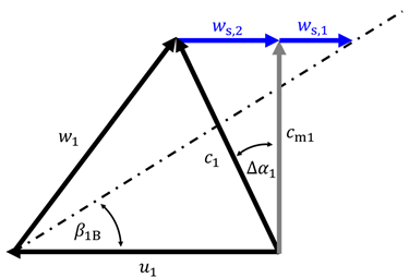
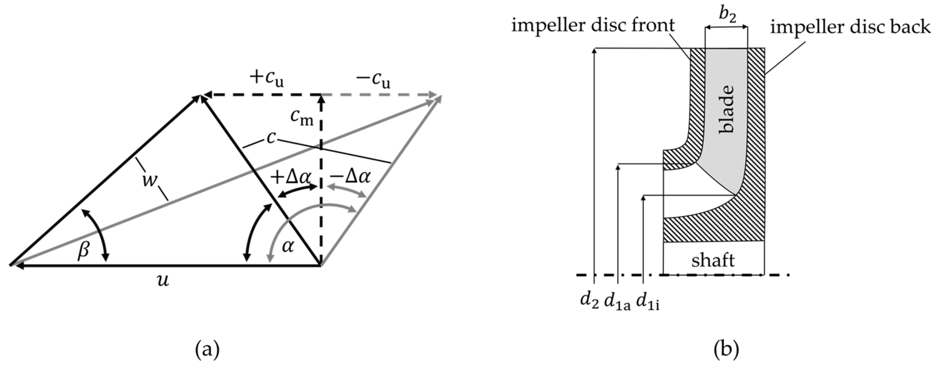
4.1. Derivation of the Model

In a previous publication, we have already derived a model for determining the specific impeller work ($\tilde{Y}$) [26]. It is calculated according to Equation (18) [26]. The angle of the impeller blade at the impeller outlet is designated as ${\beta }_{2\mathrm{B}}$. The two tuning factors, $t_0$ and $t_2$, are employed to align the specific impeller work with the respective pump.

$$\tilde{Y}=\left(\gamma +t_0-{\displaystyle \frac{Q+t_2\sqrt{H}}{\pi {\left(b d u\right)}_2}}\left(\cot \left({\beta }_{2\mathrm{B}}\right)+{\displaystyle \frac{4b_2{d}_{1,\mathrm{m}}}{d_{1\mathrm{a}}^2-d_{1\mathrm{i}}^2}}\tan \left({∆\alpha }_1\right)\right)\right)u_2^2$$

(18)

In addition to the specific hydraulic work ($Y$), the specific impeller work also encompasses the hydraulic losses that occur in the pump. As demonstrated by Equation (19), the specific hydraulic work is calculated by subtracting the total hydraulic losses from the specific impeller work. In addition to the mentioned losses in the impeller ($Z_{\mathrm{L}\mathrm{N},\mathrm{S}\mathrm{t}}, Z_{\mathrm{L}\mathrm{N},\mathrm{K}\mathrm{a}}$), losses also occur in the volute. These are divided into two categories: friction losses ($Z_{\mathrm{G}\mathrm{L},\mathrm{R}}$) and shock losses ($Z_{\mathrm{G}\mathrm{L},\mathrm{S}\mathrm{t}}$). During partial load operation, a recirculation area develops in front of the pump impeller [27]. This can result in an additional prewhirl, which typically results in a reduction in the head [27]. For this reason, partial load recirculation is considered a loss and incorporated into Equation (19) as recirculation loss ($Z_{\mathrm{R}\mathrm{e}\mathrm{z}}$).

$$Y=\tilde{Y}-Z_{\mathrm{L}\mathrm{N},\mathrm{S}\mathrm{t}}-Z_{\mathrm{L}\mathrm{N},\mathrm{K}\mathrm{a}}-Z_{\mathrm{G}\mathrm{L},\mathrm{S}\mathrm{t}}-Z_{\mathrm{G}\mathrm{L},\mathrm{R}}-Z_{\mathrm{R}\mathrm{e}\mathrm{z}}$$

(19)

In order to map the head characteristic curve using the approach outlined in Equation (19), it is necessary to model the individual loss components. The loss models are considered in accordance with physical approaches and interpretable tuning factors ($t_i$). This extends the model presented earlier [26], which considers the tuning factors $t_i\in \underset{\_}{t}, i\in \left\{0;4\right\}, i\in \mathbb{N}$ in the tuning vector ($\underset{\_}{t})$. We identified tuning factors by the Levenberg-Marquardt method with barrier terms [26], the same approach is used to identify the new tuning factors. The preceding chapters have demonstrated that the relative velocity plays an important role. This not only affects the friction losses but also the Coriolis acceleration and the associated secondary flows. This implies that the relative velocity must be incorporated into the loss models for the impeller. A methodology for modelling friction and turbulence losses was presented by J. Gülich [27]. The relationship $Z_{\mathrm{L}\mathrm{N},\mathrm{K}\mathrm{a}}\propto {w_{\mathrm{m}}}^2$ can be derived from this model. Upon consideration of the tuning factor $t_5$, the resulting equation is Equation (20). The mean relative velocity in the impeller ($w_{\mathrm{m}}$) is calculated using Equation (21) [27].

$$Z_{\mathrm{L}\mathrm{N},\mathrm{K}\mathrm{a}}=t_5{w_{\mathrm{m}}}^2$$

(20)

$$w_{\mathrm{m}}={\displaystyle \frac{w_{1,\mathrm{m}}+w_2}{2}}$$

(21)

In addition to the influence of the relative velocity on the secondary flows, an influence on the shock losses may also be determined. C. Pfleiderer developed a model for calculating the shock losses ($Z_{\mathrm{L}\mathrm{N},\mathrm{S}\mathrm{t}}$) [34], as follows:

$$Z_{\mathrm{L}\mathrm{N},\mathrm{S}\mathrm{t}}={\phi }_{\mathrm{S}\mathrm{t}}{\displaystyle \frac{{w_{\mathrm{s}}}^2}{2}}.$$

(22)

The shock factor, denoted by ${\phi }_{\mathrm{S}\mathrm{t}}$, is assumed to lie within the interval ${\phi }_{\mathrm{S}\mathrm{t}}\in \left\{0.5;0.7\right\}$ [34]. The shock velocity ($w_{\mathrm{s}}$) included in Equation (22) forms an impulse when the vector direction of the relative velocity deviates from the blade entry angle. Equation (22) and the named relationship $Z_{\mathrm{L}\mathrm{N},\mathrm{S}\mathrm{t}}\propto {w_1}^2$ [27] demonstrate the parabolic trajectory of shock losses. Nevertheless, the superimposed offset of the shock losses, as illustrated in Figure 12a, is not reflected in the models. The approach outlined in Equations (23) and (24) [26] and (25) was derived from C. Pfleiderer’s model presented in Equation (22) [34]. The expression within the square bracket in Equation (23) is based on the impact velocity ($w_{\mathrm{s}}$) for varying flow rates and the prewhirl angle ${∆\alpha }_1$. The tuning factor $t_7$ is associated with the flow rate at ${∆\alpha }_1=0°$. Furthermore, $t_6\stackrel{\wedge}{=}{\phi }_{\mathrm{S}\mathrm{t}}$ applies. The flow rate of the impeller ($\tilde{Q}$) can be modelled using Equation (24) [26]. The blockage of the flow cross-section by the blades of the impeller results in an additional shock. The offset superimposed on the shock losses is therefore interpreted as a Borda-Carnot shock loss, which is considered in Equation (23) by $Z_{\mathrm{B}\mathrm{C}}$. Modelling of $Z_{\mathrm{B}\mathrm{C}}$ is based on Equation (25). The two quadratic expressions within the brackets correspond to the quadratic relative velocity on the mean streamline without shock as a function of the prewhirl angle (${∆\alpha }_1$). A comprehensive derivation of the shock loss, as per Equations (23) and (25), can be found in Appendix B.

$$Z_{\mathrm{L}\mathrm{N},\mathrm{S}\mathrm{t}}={\displaystyle \frac{t_6}{2}}{\left(u_{1,\mathrm{m}}\left(1-{\displaystyle \frac{\tilde{Q}}{t_7}}\right)-{\displaystyle \frac{\tilde{Q}}{A_1}}\tan \left({∆\alpha }_1\right)\right)}^2+Z_{\mathrm{B}\mathrm{C}}$$

(23)

$$\tilde{Q}=Q+t_2\sqrt{H}$$

(24)

$$Z_{\mathrm{B}\mathrm{C}}=t_8\left({\left({\displaystyle \frac{u_{1,\mathrm{m}}}{\frac{u_{1,\mathrm{m}}{A}_1}{t_7}+\tan \left({∆\alpha }_1\right)}}\right)}^2+{\left(u_{1,\mathrm{m}}-{\displaystyle \frac{u_{1,\mathrm{m}}\tan \left({∆\alpha }_1\right)}{\frac{u_{1,\mathrm{m}}{A}_1}{t_7}+\tan \left({∆\alpha }_1\right)}}\right)}^2\right)$$

(25)

According to Equation (20), the friction and turbulence losses in the volute ($Z_{\mathrm{G}\mathrm{L},\mathrm{R}}$) can be calculated as follows:

$$Z_{\mathrm{G}\mathrm{L},\mathrm{R}}=t_9{Q}^2$$

(26)

The shock losses in the volute can be modelled according to Equation (27). The tuning factor $t_{11}$ represents the flow rate without shock in the volute.

$$Z_{\mathrm{G}\mathrm{L},\mathrm{S}\mathrm{t}}=t_{10}{\left(Q-t_{11}\right)}^2$$

(27)

As previously stated, partial load recirculation can result in a reduction in the head. For this purpose, the recirculation loss ($Z_{\mathrm{R}\mathrm{e}\mathrm{z}}$) was modelled by the tuning factor $t_{12}$ and the recirculation efficiency (${\eta }_{\mathrm{R}\mathrm{e}\mathrm{z}}$). A model for the recirculation efficiency has already been derived in our previous publication [26] on the basis of the sigmoid function. The recirculation efficiency can be calculated according to Equation (29) [26].

$$Z_{\mathrm{R}\mathrm{e}\mathrm{z}}=t_{12}\left(1-{\eta }_{\mathrm{R}\mathrm{e}\mathrm{z}}\right)$$

(28)

$${\eta }_{\mathrm{R}\mathrm{e}\mathrm{z}}={\displaystyle \frac{1+t_4}{1+e^{-t_3\frac{Q}{Q^{*}}}}}-t_4$$

(29)

The tuning vector $\underset{\_}{t}$ introduced previously [26] is now expanded to $t_i\in \underset{\_}{t}, i\in \left\{0;12\right\}, i\in \mathbb{N}$. Once all loss models have been incorporated into Equation (19), the head can be calculated according to Equation (30) [27].

$$H={\displaystyle \frac{Y}{g}}$$

(30)

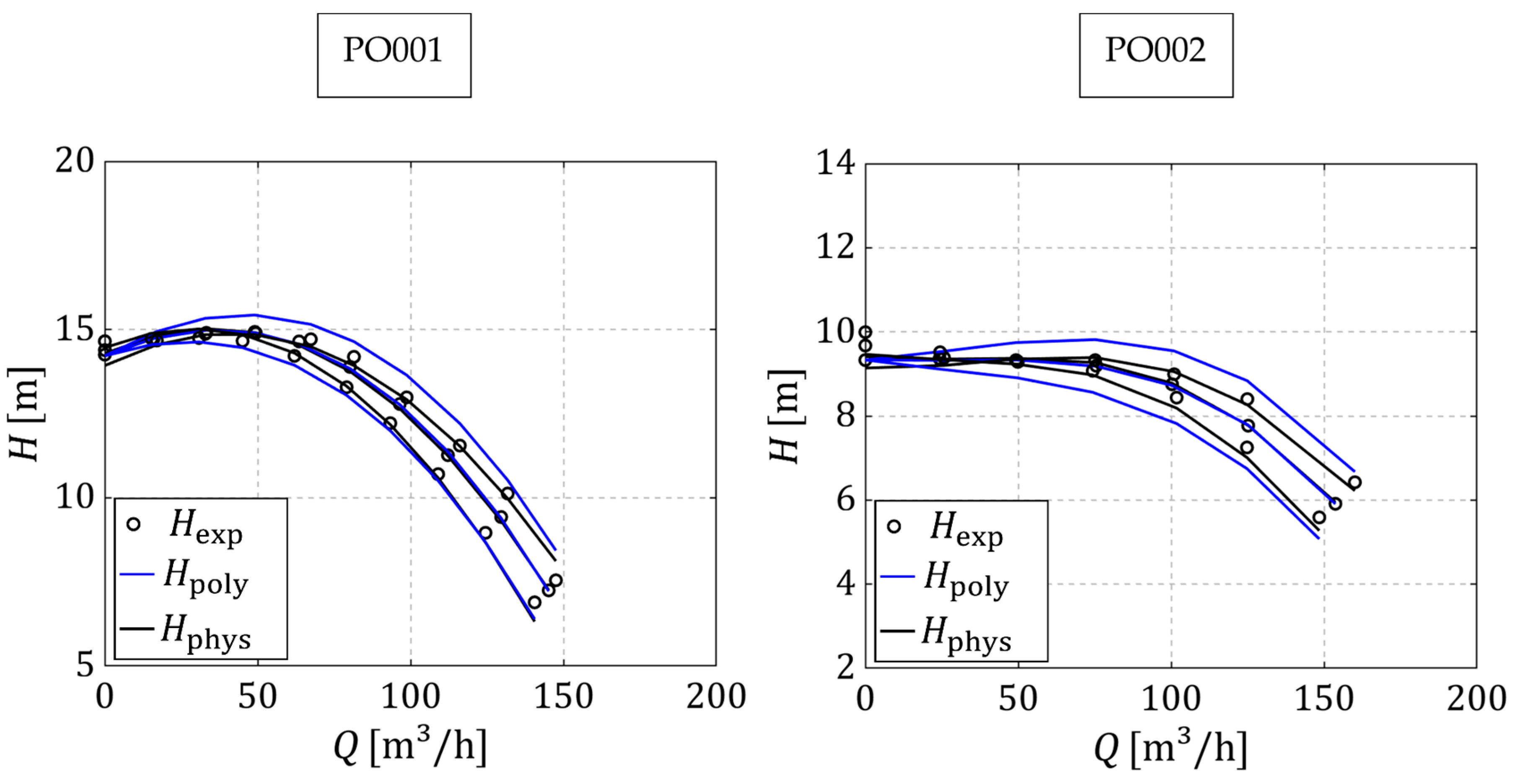
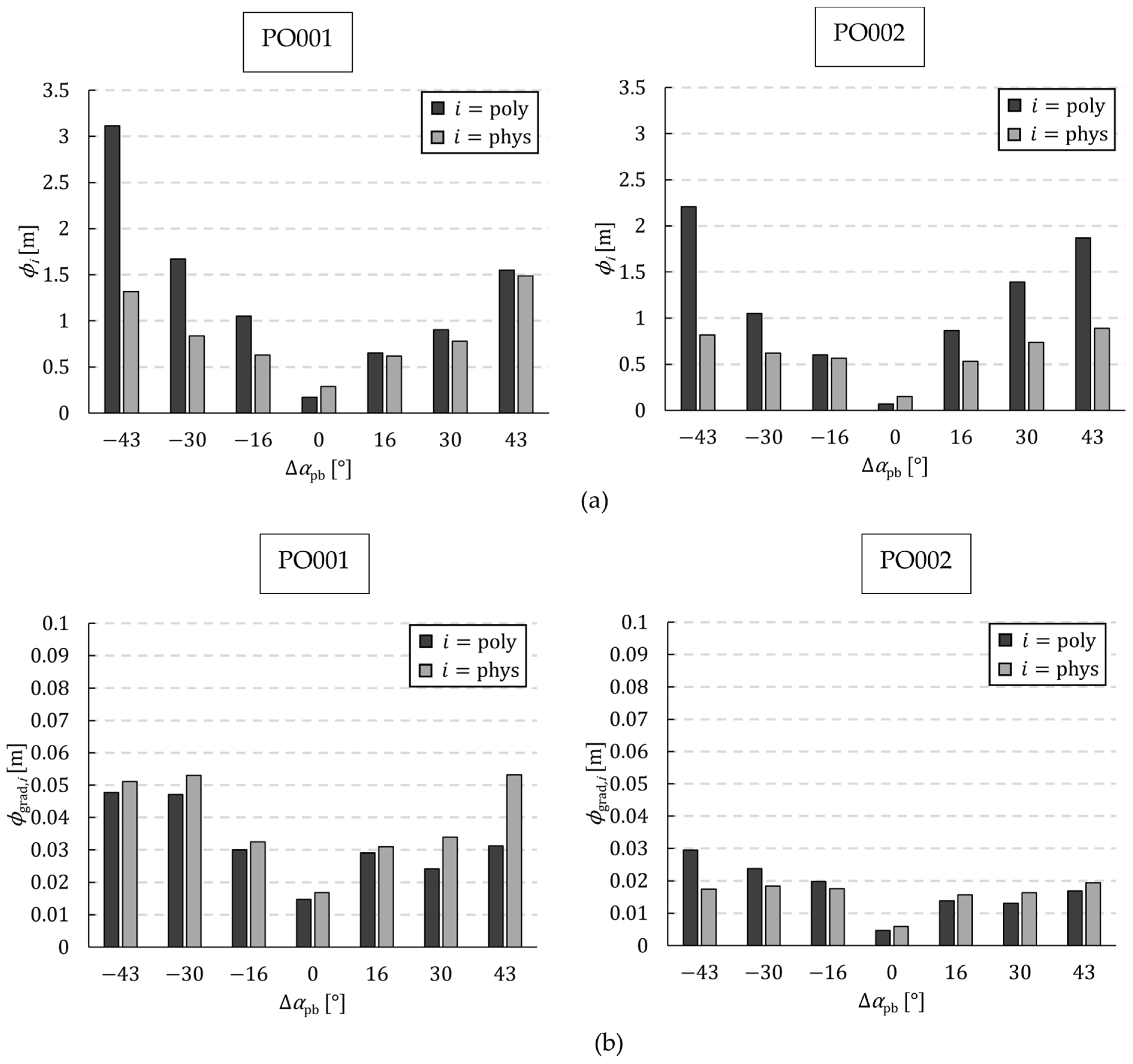
4.2. Comparison between the Models with Different Loss Treatments and the Experimental Results

The physical model derived in the previous chapter for mapping the characteristic curves of the head can be utilised to calculate the characteristic curves of radial centrifugal pumps for varying prewhirl angles. For this purpose, the experimentally determined characteristic curves of the two analysed pumps are calculated using the physical model. In contrast, the characteristic curves are calculated using an approach function based on a third-degree polynomial, without modelling the losses. The objective of this analysis is to examine the impact of the loss treatment of the derived model based on the relative velocity in greater detail. Equation (31) shows the formula used to calculate the head on a polynomial basis ($H_{\mathrm{p}\mathrm{o}\mathrm{l}\mathrm{y}}$). The letters $a,b,c$ and $d$ represent the individual coefficients of the polynomial. The right-hand term in Equation (31) is employed in order to calculate the influence of the prewhirl on the head. In Equation (31), ${\eta }_{\mathrm{S}\mathrm{p}}$ represents the volumetric efficiency used to account for gap flow losses. For this, ${\eta }_{\mathrm{S}\mathrm{p}}=0.96=\mathrm{c}\mathrm{o}\mathrm{n}\mathrm{s}\mathrm{t}.$ is assumed.

$$H_{\mathrm{p}\mathrm{o}\mathrm{l}\mathrm{y}}=a{Q}^3+b{Q}^2+cQ+d-{\displaystyle \frac{4Q{d}_{1,\mathrm{m}}{u}_2}{g{\eta }_{\mathrm{S}\mathrm{p}}\pi d_2\left(d_{1\mathrm{a}}^2-d_{1\mathrm{i}}^2\right)}}\tan \left({∆\alpha }_1\right)$$

(31)

In order to assess the deviations between the various models and the experiments, an objective functional of the respective model $i$ (${\underset{\_}{z}}_i$) is defined based on the identification of the tuning vectors by the Levenberg-Marquardt method, as outlined in Equation (32) [26]. The objective functional is a vector with length $n$. In this context, $n$ represents the number of measurement points derived from the experimental determination of the characteristic curves.

$${\underset{\_}{z}}_i≔{\left(H_{i,1}-H_{\mathrm{e}\mathrm{x}\mathrm{p},1},H_{i,2}-H_{\mathrm{e}\mathrm{x}\mathrm{p},2},\cdots ,H_{i,n}-H_{\mathrm{e}\mathrm{x}\mathrm{p},n} \right)}^T$$

(32)

To facilitate a comparative analysis of the models for different prewhirl body angles, the objective functional norm for model $i$ (${\varphi }_i$) is formed using the equation proposed by [26]:

$${\varphi }_i=‖{\underset{\_}{z}}_i‖.$$

(33)

The prewhirl angle at the impeller inlet (${∆\alpha }_1$) is required for the calculation of the characteristic curves. ${∆\alpha }_1$ was identified by CFD simulations and is presented in

Table 4. Prewhirl angle (${∆\alpha }_1$) determined by the CFD simulation as a function of the prewhirl body angle (${∆\alpha }_{\mathrm{p}\mathrm{b}}$) for PO001 and PO002.

PO001		PO002
${∆\mathit{\alpha }}_{\mathbf{p}\mathbf{b}}$	$∆{\mathit{\alpha }}_1$	${∆\mathit{\alpha }}_{\mathbf{p}\mathbf{b}}$	$∆{\mathit{\alpha }}_1$
−43°	−41.73°	−43°	−33.28°
−30°	−27.79°	−30°	−21.74°
−16°	−14.70°	−16°	−11.01°
+16°	+14.22°	+16°	+11.46°
+30°	+27.95°	+30°	+22.06°
+43°	+41.76°	+43°	+33.95°

for the investigated prewhirl body angles.

Figure 14 illustrates the characteristic curves of the head for PO001 and PO002 at the prewhirl body angles ${∆\alpha }_{\mathrm{p}\mathrm{b}}\in \left\{-30°;0°;+30°\right\}$. The characteristic curve of the experimentally determined head ($H_{\mathrm{e}\mathrm{x}\mathrm{p}}$) is represented by the circles. The blue lines represent the characteristic curves of the head, which have been calculated by the polynomial model derived from Equation (31) ($H_{\mathrm{p}\mathrm{o}\mathrm{l}\mathrm{y}}$). The black characteristic curves of the head have been calculated by the physical model derived in the previous chapter ($H_{\mathrm{p}\mathrm{h}\mathrm{y}\mathrm{s}}$). For both pumps, $H_{\mathrm{p}\mathrm{o}\mathrm{l}\mathrm{y}}$ overestimates the head, particularly for negative prewhirl angles. This is because increased hydraulic losses were not taken into account. For PO002, a deviation can also be recognized for a positive prewhirl body angle. It is assumed that the hydraulic losses are too high in this instance. The qualitative analysis indicates that the determination of the head using the derived physical model ($H_{\mathrm{p}\mathrm{h}\mathrm{y}\mathrm{s}}$) more accurately reflects the measurements.

To facilitate a quantitative comparison between the models and measurements, Figure 15a illustrates the objective functional norm, defined by Equation (33), for the two models across various prewhirl body angles. In particular, when considering the negative prewhirl body angles, it becomes evident that the physical model is capable of mapping the head characteristics with a higher degree of accuracy than the polynomial approach. As previously demonstrated in Figure 14, the physical model for PO002 also more accurately depicts the positive prewhirl body angles. In addition to the deviations, the shape accuracy of the characteristic curve determined by the models is also important. The objective functional was formed for the gradients of the models and the measurements, and their norm was demonstrated in Figure 15b. The absolute values indicate that the gradients can be mapped with minor deviations in both models. However, the physical model shows slightly poorer representations of the gradients, partly due to the approach function used to account for recirculation.

5. Conclusions

A physical model was developed to determine the characteristic curve of the head for radial centrifugal pumps. To assess the impact of varying prewhirl angles on hydraulic losses, experimental and numerical investigations were conducted. The findings from this study enabled the development of modelling approaches for the various sources of loss. As a result, it has been shown that the model can achieve higher accuracies in mapping the characteristics with prewhirl than with a polynomial-based approach. This study addressed the identified research gap by providing a mathematical description of the dependence of hydraulic losses on the pre-twist angle. The following conclusions can be drawn:

−

The hydraulic losses in radial centrifugal pumps are influenced by the prewhirl. The observed changes in losses can be attributed primarily to the pump impeller.

−

The extent of the losses depends on the sign of the prewhirl angle. Negative prewhirl angles increase hydraulic losses, while positive prewhirl angles reduce them.

−

The majority of the hydraulic losses in the impeller occur at the leading edge of the blades and in the area of the impeller outlet.

−

The degree of prewhirl angle has a significant impact on the whirl of the impeller, as well as the relative velocities. The Coriolis force increases in direct proportion to the relative velocity, which can result in the generation of secondary flows. These factors contribute to an increase in the likelihood of loss, particularly at the point of impeller inlet.

−

In addition to the secondary flows, the shock losses are also influenced by the prewhirl angles.

-

Furthermore, the relative velocities exert an influence on the friction losses in the impeller, whereby these increase with negative prewhirl angles.

−

The modelling of impeller losses based on relative velocity allows for the consideration of the differing influences of positive and negative prewhirl angles.

−

The model enhances the mapping of the characteristic curves of the head. It can therefore be utilised in the construction of soft sensors for the determination of flow rates in instances of disrupted inflows. This facilitates more accurate flow rate determination.

References

1. Sebastian, L. Nutzung des Energiesparpotentials von Kreiselpumpen Durch Szenarienbasierte Regelung; Ruhr-Universi at Bochum: Oberhausen, Germany, 2015. [Google Scholar]
2. Desborough, L.; Miller, R. Increasing Customer Value of Industrial Control Performance Monitoring—Honeywell’s Experience. In Chemical Process Control-VI: Assessment and New Directions for Research, Proceedings of the 6th International Conference on Chemical Process Control, Tucson, AZ, USA, 7–12 January 2001; AIChE Symposium Series 326; American Institute of Chemical Engineers (AIChE): New York, NY, USA, 2002; pp. 169–189. [Google Scholar]
3. Leonow, S.; Monnigmann, M. Soft Sensor Based Dynamic Flow Rate Estimation in Low Speed Radial Pumps. In Proceedings of the IEEE 2013 European Control Conference (ECC), Zurich, Switzerland, 17–19 July 2013; pp. 778–783. [Google Scholar]
4. Rakibuzzaman, M.; Suh, S.-H.; Yoon, I.-S.; Jung, S.Y. A Study on the Individual Pump Flow Estimation Processor for Optimal Operation. E3S Web Conf. 2021, 321, 02005. [Google Scholar] [CrossRef]
5. Shankar, A.; Subramaniam, U.; Madurai Elavarasan, R.; Raju, K.; Shanmugam, P. Sensorless Parameter Estimation of VFD Based Cascade Centrifugal Pumping System Using Automatic Pump Curve Adaption Method. Energy Rep. 2021, 7, 453–466. [Google Scholar] [CrossRef]
6. Roth, M. Experimentelle und numerische Untersuchung zum Einfluss von Einbaubedingungen auf das Betriebs- und Kavitationsverhalten von Kreiselpumpen. Ph.D. Thesis, Technische Universität, Darmstadt, Germany, 2006. [Google Scholar]
7. Fockert, A.; Verhaart, F.; Ferdos, F. Experimentally Determined Effect of Swirl on the Performance of a Rotodynamic Pump. J. Hydraul. Res. 2022, 60, 434–444. [Google Scholar] [CrossRef]
8. Siekmann, H. Auswirkung Ungleichmäßiger Zuströmung auf Spezifisch Schnellläufige Kreiselpumpen; TU-Berlin: Berlin, Germany, 1984; p. 250. [Google Scholar]
9. Schröder, I.V. Experimentelle Untersuchungen über Vordralleinflüsse auf die Kennlinien von Radialpumpen Verschiedener Schnellläufigkeit; ReportKönigsbrunn, Germany. 2012. Available online: https://docplayer.org/52403643-Experimentelle-untersuchungen-ueber-vordralleinfluesse-auf-die-kennlinien-von-radialpumpen-verschiedener.html (accessed on 11 January 2022).
10. Tan, L.; Cao, S.; Gui, S. Hydraulic Design and Pre-Whirl Regulation Law of Inlet Guide Vane for Centrifugal Pump. Sci. China Technol. Sci. 2010, 53, 2142–2151. [Google Scholar] [CrossRef]
11. Zhou, C.M.; Wang, H.M.; Huang, X.; Lin, H. Influence of the Positive Prewhirl on the Performance of Centrifugal Pumps with Different Airfoils. IOP Conf. Ser. Earth Environ. Sci. 2012, 15, 032020. [Google Scholar] [CrossRef]
12. Ahmed, S.A.; Muiz, A.; Mubashir, M.; Ahmed, W. Efficiency Enhancement of Centrifugal Water Pump by Using Inlet Guided Vanes. Eur. J. Adv. Eng. Technol. 2016, 3, 1–4. [Google Scholar]
13. Tan, L.; Cao, S.; Wang, Y.; Zhu, B. Influence of Axial Distance on Pre-Whirl Regulation by the Inlet Guide Vanes for a Centrifugal Pump. Sci. China Technol. Sci. 2012, 55, 1037–1043. [Google Scholar] [CrossRef]
14. Liu, Y.; Tan, L.; Liu, M.; Hao, Y.; Xu, Y. Influence of Prewhirl Angle and Axial Distance on Energy Performance and Pressure Fluctuation for a Centrifugal Pump with Inlet Guide Vanes. Energies 2017, 10, 695. [Google Scholar] [CrossRef]
15. Tan, L.; Zhu, B.; Cao, S.; Wang, Y.; Wang, B. Influence of Prewhirl Regulation by Inlet Guide Vanes on Cavitation Performance of a Centrifugal Pump. Energies 2014, 7, 1050–1065. [Google Scholar] [CrossRef]
16. Wu, W.; Wang, Y.; Han, Y.W. Impeller Entrance Pre Whirl Characteristics Research. IOP Conf. Ser. Mater. Sci. Eng. 2016, 129, 012026. [Google Scholar] [CrossRef]
17. Hou, H.; Zhang, Y.; Li, Z.; Zhou, X.; Wang, Z. Hydraulic Design of Inlet Guide Vane and Its Full Flow Passage Numerical Simulation on Centrifugal Pump. In Proceedings of the Volume 7: Fluids Engineering Systems and Technologies, American Society of Mechanical Engineers, Montreal, QC, Canada, 14 November 2014; p. V007T09A072. [Google Scholar]
18. Zibin, X. Study on the H-Q Characteristic Curves of Centrifugal Pump with Inlet Pre-Whirl. In Proceedings of the IEEE 2015 Sixth International Conference on Intelligent Systems Design and Engineering Applications (ISDEA), Guiyang, China, 18–19 August 2015; pp. 763–766. [Google Scholar]
19. Lin, P.; Li, Y.; Xu, W.; Chen, H.; Zhu, Z. Numerical Study on the Influence of Inlet Guide Vanes on the Internal Flow Characteristics of Centrifugal Pump. Processes 2020, 8, 122. [Google Scholar] [CrossRef]
20. Song, P.; Wei, Z.; Zhen, H.; Liu, M.; Ren, J. Effects of Pre-Whirl and Blade Profile on the Hydraulic and Cavitation Performance of a Centrifugal Pump. Int. J. Multiph. Flow 2022, 157, 104261. [Google Scholar] [CrossRef]
21. Ma, X.; Bian, M.; Yang, Y.; Dai, T.; Tang, L.; Wang, J. Study on the Effect Mechanism of Inlet Pre-Swirl on Pressure Pulsation within a Mixed-Flow Centrifugal Pump. Water 2023, 15, 1223. [Google Scholar] [CrossRef]
22. Li, H.; Chen, Y.; Yang, Y.; Wang, S.; Bai, L.; Zhou, L. CFD Simulation of Centrifugal Pump with Different Impeller Blade Trailing Edges. J. Mar. Sci. Eng. 2023, 11, 402. [Google Scholar] [CrossRef]
23. Zhang, C.; Pei, J.; Wang, W.; Yuan, S.; Gan, X.; Huang, C.; Chen, J. Unsteady Simulation and Analysis of Energy Loss Mechanism of a Vertical Volute Pump Under Stall Conditions. J. Fluids Eng. 2023; 145, 081201. [Google Scholar] [CrossRef]
24. Wang, H.; Yang, Y.; Xi, B.; Shi, W.-D.; Wang, C.; Ji, L.-L.; Song, X.-Y.; He, Z.-M. Inter-Stage Performance and Energy Characteristics Analysis of Electric Submersible Pump Based on Entropy Production Theory. Pet. Sci. 2023, 21, 1354–1368. [Google Scholar] [CrossRef]
25. Yang, Y.; Chen, X.; Bai, L.; Wang, H.; Ji, L.; Zhou, L. Energy Performance Prediction Model for Mixed-Flow Pumps by Considering the Effect of Incoming Prerotation. J. Fluids Eng. 2024, 146, 061204. [Google Scholar] [CrossRef]
26. Reeh, N.; Manthei, G.; Klar, P.J. Physical Modelling of the Set of Performance Curves for Radial Centrifugal Pumps to Determine the Flow Rate. Appl. Syst. Innov. 2023, 6, 111. [Google Scholar] [CrossRef]
27. Gülich, J.F. Kreiselpumpen, Handbuch Für Entwicklung, Anlagenplanung Und Betrieb; 5. Auflage; Springer Vieweg: Villeneuve, Switzerland, 2020; ISBN 978-3-662-59784-2. [Google Scholar]
28. Limbach, P.; Müller, T.; Blume, M.; Skoda, R. Numerical and Experimental Investigation of the Cavitating Flow in a Low Specific Speed Centrifugal Pump and Assessment of the Influence of Surface Roughness on Head Prediction. In Proceedings of the 16th International Symposium on Transport Phenomena and Dynamics of Rotating Machinery, Honolulu, NI, USA, 10–15 April 2016. [Google Scholar]
29. CFX-Solver Theory Guide. ANSYS, Inc.: Canonsburg, PA, USA, 2022.
30. Menter, F.R. Two-Equation Eddy-Viscosity Turbulence Models for Engineering Applications. AIAA J. 1994, 32, 1598–1605. [Google Scholar] [CrossRef]
31. Herwig, H.; Kock, F. Direct and Indirect Methods of Calculating Entropy Generation Rates in Turbulent Convective Heat Transfer Problems. Heat Mass Transf. 2007, 43, 207–215. [Google Scholar] [CrossRef]
32. Ji, L.; Li, W.; Shi, W.; Tian, F.; Agarwal, R. Effect of Blade Thickness on Rotating Stall of Mixed-Flow Pump Using Entropy Generation Analysis. Energy 2021, 236, 121381. [Google Scholar] [CrossRef]
33. Brun, K.; Kurz, R. Analysis of Secondary Flows in Centrifugal Impellers. Int. J. Rotating Mach. 2005, 2005, 856141. [Google Scholar] [CrossRef]
34. Pfleiderer, C. Die Kreiselpumpen für Flüssigkeiten und Gase: Wasserpumpen, Ventilatoren, Turbogebläse, Turbokompressoren, 4th ed.; Springer: Berlin/Heidelberg, Germany, 1955; ISBN 978-3-642-48171-0. [Google Scholar]
Figure 1. Flowchart illustrating the research methodology, divided into the two main branches of experimental analysis and CFD analysis.
Applsci 14 07224 g001
Figure 2. (a) Velocity triangle of the impeller showing the different velocity components at positive (black lines) and negative (grey lines) whirl angles ( α ); (b) meridian view of the impeller for a radial centrifugal pump and geometrical parameters, where the index 1 denotes the blade inlet and 2 the blade outlet.
Applsci 14 07224 g002
Figure 3. The experimental setup with the variables that are measured in order to obtain the characteristic curves at varying prewhirl body angles ( α p b ), which are imposed on the inflow by prewhirl bodies as described in [26].
Applsci 14 07224 g003
Figure 4. (a) The three-dimensional geometry of the flow area for PO001 is presented in side view, comprising the inlet pipe, prewhirl body, inlet housing, gap, front side gap, volute, back side gap, and outlet pipe; (b) the three-dimensional geometry of the flow area for PO001 is presented in front view, without the inlet pipe, side gaps, gap and outlet pipe with volute, interface and impeller.
Applsci 14 07224 g004
Figure 5. (a) Nature of the mesh around the tongue of the volute; (b) surface meshes of the prewhirl bodies and impeller with the prewhirl body hub.
Applsci 14 07224 g005
Figure 6. (a) Total flow area with details of the boundary conditions (boundary inlet and boundary outlet); (b) equivalent sand grain roughness ( k s ) at the wall boundary conditions for the prewhirl body, the impeller and the prewhirl body hub.
Applsci 14 07224 g006
Figure 7. Characteristic curves of the head ( H e x p ) plotted against the flow rate ( Q e x p ) for PO001 (top figure) and PO002 (bottom figure) with varying motor frequencies ( f M ) and varying inflow without ( α p b = 0 ° ), with positive ( α p b > 0 ° ) and with negative ( α p b < 0 ° ) prewhirl angles.
Applsci 14 07224 g007
Figure 8. Ratio of the static pressure at the pressure side ( p p s , e x p ) to the static pressure in the back side gap ( p R S R , e x p ) with varying motor frequencies ( f M ) and varying inflow without ( α p b = 0 ° ), with positive ( α p b > 0 ° ) and negative ( α p b < 0 ° ) prewhirl angles.
Applsci 14 07224 g008
Figure 9. Comparison of the head ( H ) (left-hand side) and the power consumption ( P 2 ) (right-hand side) between the experimental results (Exp) and the simulation (CFD) for the prewhirl body angles α p b 30 ° ; 0 ° ; + 30 ° .
Applsci 14 07224 g009
Figure 10. (a) Hydraulic power loss in the volute for the prewhirl body angle α p b 30 ° ; 0 ° ; + 30 ° ; (b) hydraulic power loss in the impeller for the prewhirl body angle α p b 30 ° ; 0 ° ; + 30 ° .
Applsci 14 07224 g010
Figure 11. (a) Mass flow averaged whirl ( u c u ¯ ) along the dimensionless streamline length ( s ) for the prewhirl body angles α p b 30 ° ; 0 ° ; + 30 ° at Q = 100 m 3 h ; (b) mass flow averaged relative velocity ( w ¯ ) along the dimensionless streamline length ( s ) for the prewhirl body angles α p b 30 ° ; 0 ° ; + 30 ° at Q = 100 m 3 h ; (c) mass flow averaged entropy production ( S p r o ¯ ) along the dimensionless streamline length ( s ) for the prewhirl body angles α p b 30 ° ; 0 ° ; + 30 ° at Q = 100 m 3 h ; (d) area-averaged modified Rossby number ( R o m ¯ ) along the dimensionless streamline length ( s ) for the prewhirl body angles α p b 30 ° ; 0 ° ; + 30 ° at Q = 100 m 3 h .
Applsci 14 07224 g011
Figure 12. (a) Power loss due to the shock loss ( P l o s s , S t ) over the mass flow-averaged relative velocity at the impeller inlet ( w 1 ¯ ) for the three prewhirl body angles α p b 30 ° ; 0 ° ; + 30 ° ; (b) leakage flow ( Q S p ) in the gap plotted against the root of the head ( H ) for the three prewhirl body angles α p b 30 ° ; 0 ° ; + 30 ° .
Applsci 14 07224 g012
Figure 13. Entropy production ( S p r o ) on the blade sections in the area of the hub (span 0.1), the mean meridian streamline (span 0.5) and the shroud (span 0.9) for the prewhirl body angles α p b 30 ° ; 0 ° ; + 30 ° at Q = 100 m 3 h .
Applsci 14 07224 g013
Figure 14. Comparison of the characteristic curves of PO001 and PO002 between the experimentally determined head ( H e x p ) and the heads calculated by the models ( H p o l y and H p h y s ) for three prewhirl body angles α p b 30 ° ; 0 ° ; + 30 ° .
Applsci 14 07224 g014
Figure 15. (a) Norm of the objective functional ( ϕ i ) of the individual models plotted against the investigated swirl body angles ( α p b ) of PO001 and PO002; (b) norm of the objective functional of the gradient ( ϕ g r a d , i ) of the individual models plotted over the investigated prewhirl body angles ( α p b ) of PO001 and PO002.
Applsci 14 07224 g015