Advanced Industrial Fault Detection: A Comparative Analysis of Ultrasonic Signal Processing and Ensemble Machine Learning Techniques

Abstract

Modern condition monitoring and industrial fault prediction have advanced to include intelligent techniques, aiming to improve reliability, productivity, and safety. The integration of ultrasonic signal processing with various machine learning (ML) models can significantly enhance the efficiency of industrial fault diagnosis. In this paper, ultrasonic data are analyzed and applied to ensemble ML algorithms. Four methods for reducing dimensionality are employed to illustrate differences among acoustic faults. Different features in the time domain are extracted, and predictive ensemble models including a gradient boosting classifier (GB), stacking classifier (Stacking), voting classifier (Voting), Adaboost, Logit boost (Logit), and bagging classifier (Bagging) are implemented. To assess the model’s performance on new data during experiments, k-fold cross-validation (CV) was employed. Based on the designed workflow, GB demonstrated the highest performance, with less variation over 5 cross-folds. Finally, the real-time capability of the model was evaluated by deployment on an ARM Cortex-M4F microcontroller (MCU).

1. Introduction

The current manufacturing and industrial landscapes have witnessed significant growth, fostering the pervasive adoption of automated processes and a heightened need for sophisticated equipment and machinery. With the rise of industrial automation, motors and pipelines spare parts have become integral to machine maintenance. Condition monitoring for fault detection is essential for the safety of the environment, energy conservation, and human health [1,2]. The interdependence of motors and pipelines in industrial settings is crucial for overall system efficiency and safety. In industries like chemical processing, motors drive pumps that circulate fluids through pipelines. A fault in either component can disrupt the process, affecting efficiency and safety. Identifying faults in both motors and pipelines allows for a comprehensive approach to predictive maintenance, preventing downtime, optimizing maintenance schedules, and enhancing reliability. Failures in motors and pipelines are often interconnected; for example, a pipeline blockage can increase the motor load, leading to overheating and failure. Conversely, motor failure can cause pressure build-up in pipelines. This interdependence is critical in sectors like oil and gas, where component failure can lead to significant production losses and environmental hazards. Compliance with safety standards requires monitoring all critical components, as seen in the pharmaceutical industry, where motor and pipeline integrity is vital for product quality. Examples from the food and beverage industry show that faults in these components can cause contamination and safety hazards, highlighting the need for integrated fault detection systems [3,4]. This study explores prevalent issues in industrial pipes and motors, focusing on using ultrasonic methods to detect and assess problems like leaks, blockages, and flaws in underground pipes. Pipes are vital for fluid transport over various distances. The vast networks of pipelines stretching for kilometers consist of pipe sections connected by joints. External pressures such as traffic and surface loads can stress these pipes and joints, possibly causing leaks and bursts.

The increase in pipeline defects such as cracks, cavitation, corrosion, and various mechanical damages is a major concern for the safety and functionality of pipeline systems. These defects can compromise the integrity of pipelines, leading to potential hazards and disruptions to operations [5,6]. Mechanical components, particularly in rotor-bearing systems, are prone to wear and failure, often due to bearing faults. These faults can lead to significant machinery downtime and require maintenance or replacement to ensure continued operation [7]. Indeed, diagnosing faults in industrial systems is a crucial aspect of condition-based maintenance. Maintenance engineers focus on this to prevent severe breakdowns, ensuring the systems’ safety and reliability. Timely identification and repair of such faults can avert disastrous failures and maintain operational continuity [8,9]. In addition, ultrasonic fault detection offers high sensitivity for early issue identification, versatility in various applications, and non-destructive testing capabilities [10].

Various studies are conducted for the detection of industrial faults. Acoustic analysis and temperature sensing are long-standing technologies used in monitoring industrial equipment for faults. By effectively preventing equipment failures, these technologies can greatly lower maintenance expenses and reduce periods of inactivity, enhancing overall operational efficiency [11].

The research by Avendano et al. [12] combined the dyadic Wavelet transform with the Welch–Bartlett periodogram for effective feature extraction from noisy signals. Lin et al. [13] used FFT techniques to analyze vibration signals in unbalanced rolling bearings, revealing characteristic fault frequencies. Vishwendra et al. [14] applied a K-nearest neighbor (KNN) method to detect rolling element bearing faults using kurtosis and envelope spectrum analysis. Patil et al. [15] used dimensional analysis and a central composite rotatable design to identify faults in nonlinear rotating systems, focusing on the influence of bearing clearance and external defects on vibration characteristics.

A comprehensive study on leak detection and localization in oil and gas pipelines was presented in [16], reviewing various methods, their benefits, limitations, and effectiveness. The authors reviewed different methods, evaluating their advantages, drawbacks, and effectiveness in detecting and pinpointing leaks within pipeline systems. Korlapati et al. [17] evaluated multiple leak detection methods, discussing their strengths, weaknesses, and areas for future improvement. Rai et al. [18] tackled the issue of the limited historical pipeline failure data in AI methods by introducing a health index approach integrating the Kolmogorov–Smirnov test, multiscale analysis, and a Gaussian mixture model (GMM). In another experiment, Wang et al. [19] classified defects in pipeline welds using the total focusing method (TFM) based on ultrasonic phased arrays, improving defect detection and characterization. They applied the HOG–Poly–SVM algorithm with ten-fold cross-validation for defect classification. In [20], we presented a method for detecting industrial faults using ultrasonic signals by stacking an ensemble of classifiers.

Raišutis et al. [21] presented a technique using ultrasonic guided waves (UGW) with helical wave modes to detect corrosion-type defects in steel pipes. They demonstrated that phase delay differences in wave signal peaks can effectively identify defects with minimal transducers and measurements. Norli et al. [22] presented an experimental study on detecting stress corrosion cracks (SCC) in gas pipelines using guided waves and broadband ultrasound. The study successfully demonstrated the feasibility of an ART-scan-based setup for detecting SCC in a submerged pipe section, showing significant signal differences for cracks with depths of around 35% of the pipe wall thickness. Wei et al. [23] introduced a method combining a fractional Fourier transform (FRFT) and variational modal decomposition (VMD) to detect pipeline defects using ultrasonic signals. The method significantly improved feature extraction and classification accuracy, achieving 89.1% for experimental signals. Yu et al. [6] presented the application of acoustic and ultrasonic methods to detect leaks, blockages, and defects in buried water and sewerage pipes. They reviewed various sensors, including accelerometers, hydrophones, and fiber optics, and explored the potential of autonomous robotics for deploying these sensors. The paper also highlighted data-driven techniques and machine learning for enhancing the accuracy and efficiency of pipe condition assessments. Cai et al. [24] presented a method to carry out pipeline declination inspections using amplitude reduction analysis of ultrasonic echo signals. This method enhanced the detection accuracy, identifying declinations with a maximum error of 0.137° within a 2° range.

However, these works faced limitations related to environmental influences, computational time, and accuracy. These limitations highlight the ongoing need for advancements in ultrasonic inspection techniques to enhance their reliability and practical applicability in diverse and real-world conditions. This work improves upon the limitations of previous studies by offering a higher accuracy, better computational efficiency, and practical real-time deployment in ultrasonic fault detection for industrial applications. This research covers ten unique fault types in both pipelines and rotating machinery. We compare dimensionality reduction techniques and ensemble classifiers to find the best model for real-time fault detection on an MCU. To address the challenge of high-dimensional data, statistical features are extracted. Subsequently, several well-established classification models including voting, logit, GB, Adaboost, stacking, and bagging are implemented. For further investigation, dimensionality reduction techniques like principal component analysis (PCA), linear discriminant analysis (LDA), independent component analysis (ICA), and uniform manifold approximation and projection (UMAP) are analyzed. These techniques can simplify complex datasets by reducing the number of variables under consideration, while still preserving the essential structures within the data. Finally, two different approaches for MCU implementation are investigated. While previous studies have explored ultrasonic fault detection, few have integrated real-time processing on resource-constrained devices like the ARM Cortex-M4F MCU used here.

The remainder of the paper is structured as follows: Section 2 provides a description of the ultrasonic fault diagnosis methodology, and details the preprocessing, feature extraction, and used methods. Section 3 and Section 4 present the experimental results and the conclusions, respectively.

2. Ultrasonic Fault Detection Methodology

This section describes the methodologies and tools used to achieve the study’s objectives. Figure 1 provides an overview of the proposed methodology, which consists of seven main steps. Our process starts with gathering raw ultrasonic data using a microphone array module for classification analysis. Following refinement through preprocessing steps like filtering and scaling, we then extract features to generate a concise and informative feature vector. This research uses various time-domain and static-domain features based on the mean, variance, zero crossing, envelope, crest factor, shape factor, maximum number of peaks, time of peak, skewness, and kurtosis extracted from the refined ultrasonic profile. The details of these features are illustrated in

Table 1. Feature definitions and their details.

Features	Details	Definition
Mean	Mean	Average of the data.
	Median	The middle value of the signal.
	RMS (Root Mean Square)	The square root of the mean of the squares of the signal values.
Variance	Standard Deviation	The square root of the variance.
	Range	The difference between the maximum and minimum values of the signal.
	Interquartile Range (IQR)	The difference between the 75th and 25th percentiles of the signal.
Zero Crossing	Number of Peaks	The total count of peaks in the signal.
	Number of Valleys	The total count of valleys in the signal.
	Peak-to-Peak Distance	The average distance between consecutive peaks.
Envelope	Envelope Mean	The mean value of the signal envelope.
	Envelope Variance	The variance of the signal envelope.
	Envelope Energy	The sum of the squared values of the signal envelope.
Crest Factor	Form Factor	The ratio of the RMS value to the mean absolute value.
	Peak-to-RMS Ratio	The ratio of the maximum value to the RMS value of the signal.
	Margin Factor	The ratio of the maximum value to the RMS value.
Shape Factor	Normalized Energy	The energy normalized by the length of the signal.
	Energy Entropy	The logarithm of the energy of the signal.
	Impulse Factor	The ratio of the maximum value to the mean of the absolute values of the signal.
Number of Peaks	Number of Positive Peaks	The count of positive peaks in the signal.
	Number of Negative Peaks	The count of negative peaks in the signal.
	Peak Amplitude	The amplitude of the highest peak in the signal.
Time of Peak	Time of First Peak	The time at which the first peak occurs.
	Time of Last Peak	The time at which the last peak occurs.
	Time of Median	The time index of the median value.
Skewness	Absolute Skewness	Skewness calculated on the absolute values of the signal.
	Skewness of Positive Values	Skewness calculated only for the positive values of the signal.
	Skewness of Negative Values	Skewness calculated only for the negative values of the signal.
Kurtosis	Absolute Kurtosis	Kurtosis calculated on the absolute values of the signal.
	Kurtosis of Positive Values	Kurtosis calculated only for the positive values of the signal.
	Kurtosis of Negative Values	Kurtosis calculated only for the negative values of the signal.

. To address the issue of high dimensionality in raw data, which can hinder predictive modeling for ML models, dimensionality reduction techniques are applied. Finally, an ML classification algorithm is used to categorize the data. The train–test split procedure with k-fold CV is used to evaluate the performance of ensemble learning algorithms by assessing their predictions on unseen data during model training. Finally, the model can be deployed on an MCU.

High dimensionality can refer to datasets with a large number of features and classes, where numerous characteristics are derived from each signal. By increasing the number of features, the dimensionality can increase, and the complexity of the model also increases, which may lead to longer training times and higher computational resource requirements. Furthermore, with higher dimensions, models can become more prone to overfitting, especially if the number of samples is relatively small compared to the number of features. Proper dimensionality strikes a balance between retaining sufficient information for accurate predictions and reducing complexity to enhance learning efficiency. Techniques like PCA, LDA, ICA, and UMAP are employed to achieve this balance, to effectively capture the essential structure of the ultrasonic signals while reducing dimensionality.

Ensemble learning is an ML approach aimed at improving predictive performance by aggregating predictions from multiple base models. Ensemble classifiers may be more advantageous than deep learning models in situations where factors such as interpretability, limited data, computational resources, model complexity, robustness to overfitting, result reliability, lower memory occupation, and domain expertise are crucial considerations [25,26]. These fields of study have led to numerous specialized techniques including bagging, stacking, and boosting approaches.

2.1. Boosting Technique

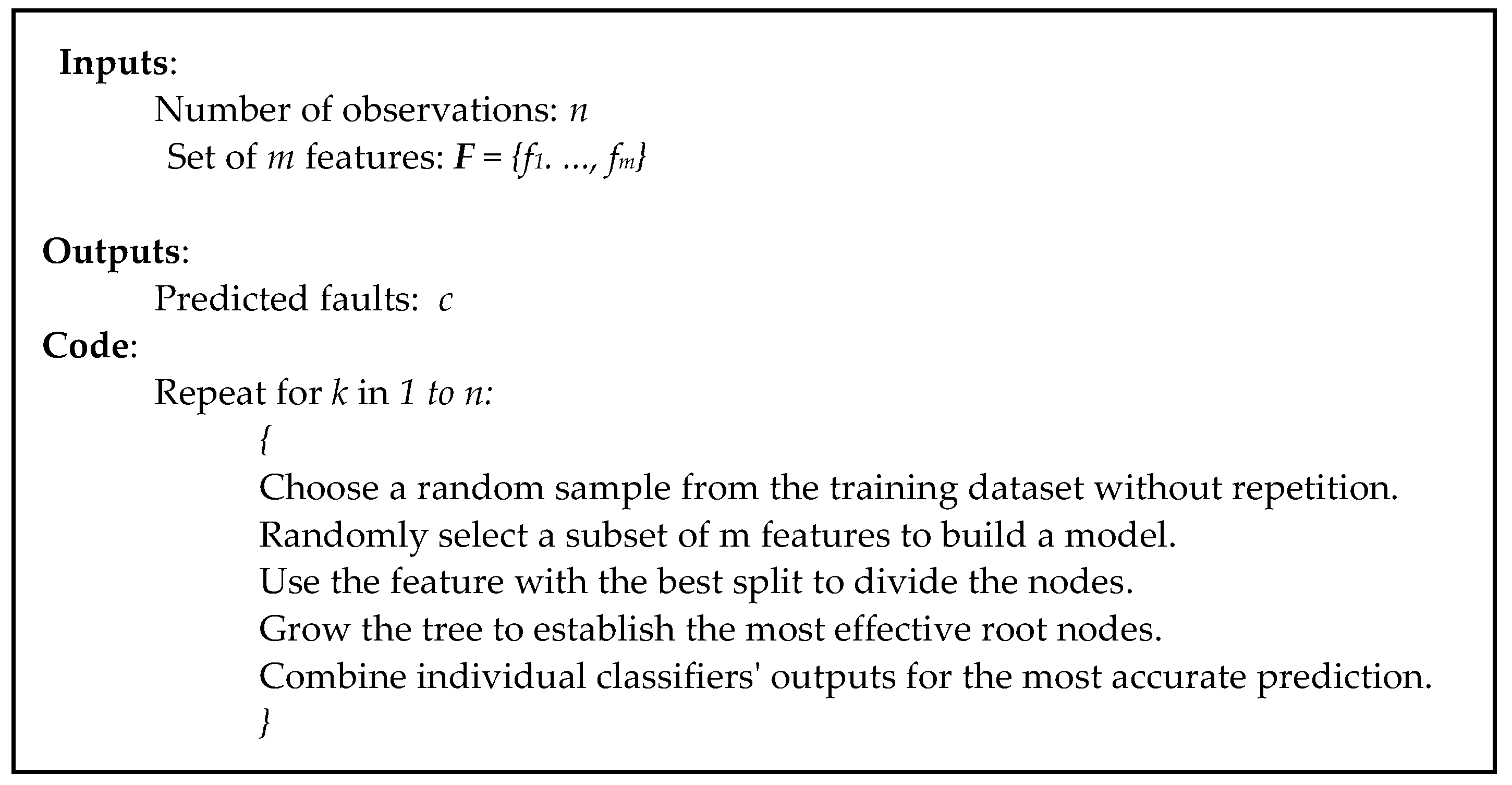
A boosting classifier is an ensemble technique that improves model accuracy by combining multiple learners. It sequentially trains each learner to correct the errors of the previous ones [27]. The algorithm starts by initializing a model, then iteratively computes residuals, fits new weak learners, determines optimal step sizes, and updates the model. After all iterations, the final boosted model is produced, yielding a high accuracy and robustness against overfitting. Boosting is robust to overfitting and versatile for various applications [28]. Adaboost, GB, and Logit are investigated in this paper. Adaboost emphasizes misclassified instances by adjusting their weights. GB uses gradient descent to minimize a chosen loss function, focusing on residuals. Logit targets logistic regression, minimizing logistic loss for improved classification. The algorithm is summarized in Figure 2.

Where n is the number of observations, m is the number of features, F is the set of m features, c is the predicted faults, $y_i$ is the actual value for observation i, $\rho$ is the parameter for initialization, $G_0(·)$ is the initial model which minimizes the loss function over all observations, $L(·)$ is the loss function which measures the error between the actual value $y_i$ and the predicted value $G(·)$, ${\tilde{y}}_i(·)$ the residuals computed for each observation i at step k, $h(·)$ is the fitted model, ${\alpha }_k$ is the model parameter at step k, ${\rho }_k$ is the gradient step size at step k, and $G_k(·)$ is the regression model at step k.

2.2. Bagging Technique

A bagging (bootstrap aggregating) classifier is an ensemble learning technique designed to improve the accuracy and robustness of machine learning models by reducing variance and preventing overfitting. The process involves creating multiple versions of a predictor by training each on a random subset of the data, then combining their predictions to form a final output. The bagging method addresses the bias and variance trade-off and mitigates the variance of the final prediction model, thereby reducing the risk of overfitting, particularly in the context of ultrasonic data [29]. The algorithm is summarized in Figure 3.

2.3. Stacking Technique

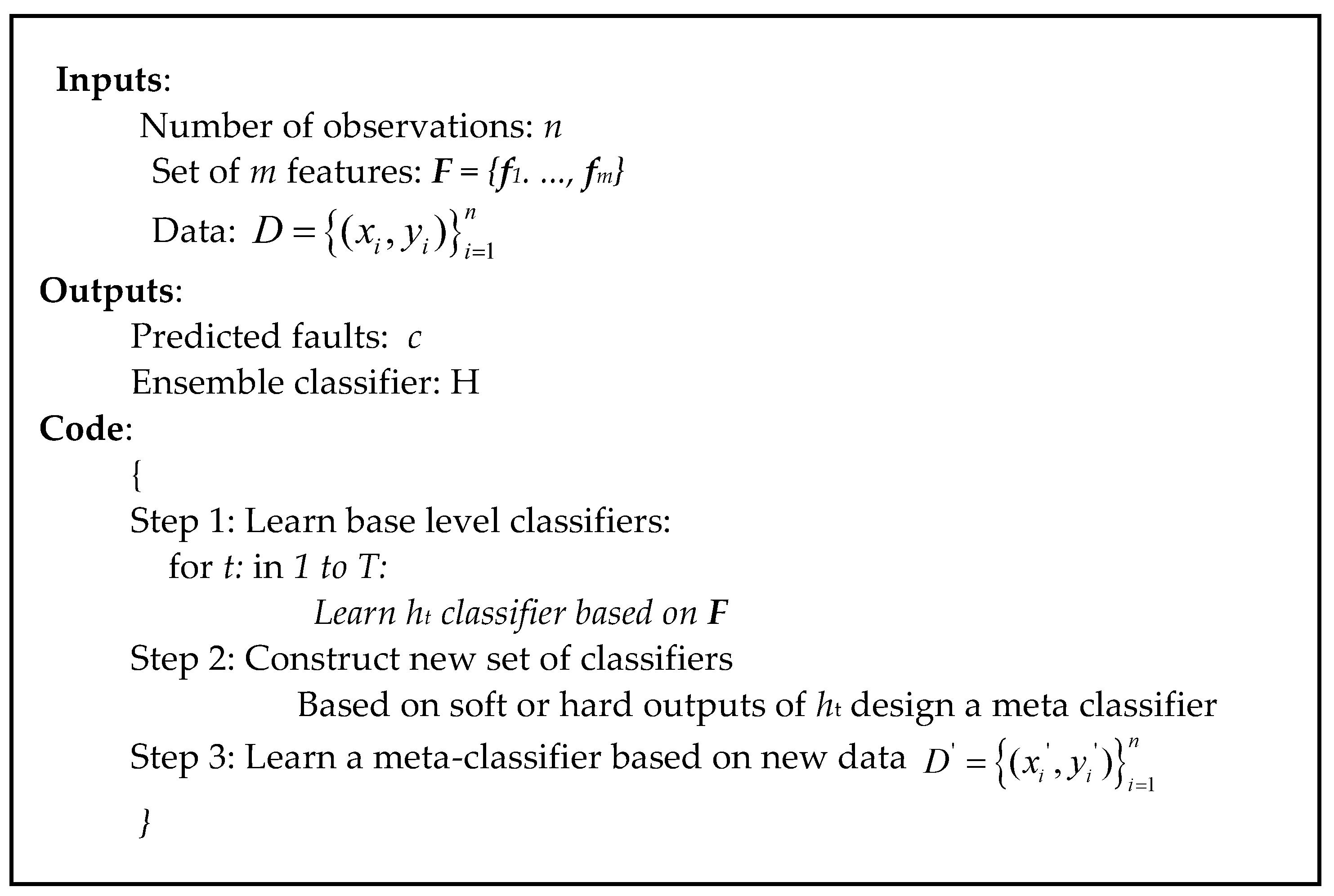
A stacking classifier is an ensemble learning technique that improves predictive performance by combining multiple base models and a meta-model. Base classifiers are trained on the same dataset and their predictions are used to train a meta-classifier. This meta-classifier learns to optimally combine the base classifiers’ outputs. Stacking leverages model diversity, improving the accuracy and robustness [30]. The algorithm is summarized in Figure 4.

Where D is the dataset, and T is the number of base level classifiers.

2.4. Evaluating Estimator Performance Using k-Fold Cross-Validation

The effectiveness of the algorithm is evaluated using k-fold cross-validation (k-fold CV), also known as rotation estimation, to verify the generalizability of the results in industrial fault detection analysis [31]. This method is used to assess a model’s performance by splitting data into k subsets. It trains the model on k − 1 subset and validates it on the remaining subsets, repeating this k times to ensure a thorough evaluation. The steps for k-fold CV are outlined in Figure 5.

To determine the optimal value of k, it is important to note that reducing the value of k decreases the size of the training dataset and increases the size of the test dataset (e.g., $k=3$ results in a 66% training dataset). This reduction can hinder the model’s ability to learn effectively. Conversely, increasing the value of k decreases the sizes of the test sets (e.g., $k=10$ results in a 10% test dataset), potentially increasing the variance of the accuracy [32,33]. In this study, the optimized split is considered as $k=5$ for k-fold CV.

2.5. Ultrasonic Dimensionality Reduction and Visualization Techniques

Dimensionality reduction in ML is a technique used to reduce the number of input features or variables in a dataset. This process simplifies the dataset by transforming it into a lower-dimensional space, while preserving as much of the important information as possible. The main reasons for using dimensionality reduction includes improving model performance, reducing overfitting, and enhancing data visualization [34,35]. Methods include the following:

• Principal component analysis (PCA) reduces the dimensionality of a dataset by transforming it into a set of orthogonal components. These components capture the most variance from the original data [36].
• Independent component analysis (ICA) separates a multivariate signal into independent non-Gaussian components, assuming statistical independence. ICA excels in identifying independent sources and handling non-Gaussian data, making it useful for noise reduction, feature extraction, and source separation [37].
• Uniform manifold approximation and projection (UMAP) preserves the local and global data structure by optimizing a low-dimensional graph to reflect the high-dimensional graph. It is computationally efficient and scalable, suitable for large datasets [38].
• Linear discriminant analysis (LDA): This is a statistical method used in supervised classification problems. LDA aims to find a linear combination of features that best separates industrial faults. It projects high-dimensional acoustic data onto a lower-dimensional space by maximizing the distance between the means of different classes and minimizing the variance within each class [39].

By applying these algorithms, we can gain insights into the patterns and relationships within the ultrasonic signals, which can be crucial for identifying anomalies or understanding the underlying physical phenomena.

2.6. Evaluation Metrics

In order to measure the performance of the proposed framework in fault detection, we employ typical quality metrics of precision, recall, F-measure, and accuracy as follows [40]:

$$\mathrm{Precision}={\displaystyle \frac{TP}{TP+FP}}$$

(1)

$$\mathrm{Recall}={\displaystyle \frac{TP}{TP+FN}}$$

(2)

$$\mathrm{F}1-\mathrm{measure}=2·{\displaystyle \frac{\mathrm{Precision}·\mathrm{Recall}}{\mathrm{Precision}+\mathrm{Recall}}}$$

(3)

$$\mathrm{Accuracy}={\displaystyle \frac{TP+TN}{TP+TN+FP+FN}}$$

(4)

where TP, FN, TN, and FP are true-positive, false-negative, true-negative, and false-positive respectively. Receiver operating characteristics (ROC) plots are visually appealing and provide an overview of a classifier’s performance across a wide range of specificities. For further investigation in this research, the classifiers are also evaluated with ROC plots.

3. Results

As discussed in the introduction, bearing and pipe faults in industrial mechanisms are often caused by a variety of factors.

The dataset used in this study was obtained from UE Systems Co. [41] with 10 categories: 4 bearing conditions and 6 pipeline conditions. The dataset of 20,000 samples was split into 80% for training and 20% for testing, enhanced by applying a sliding window with data augmentation including rotating, flipping, and adding noise to the original data.

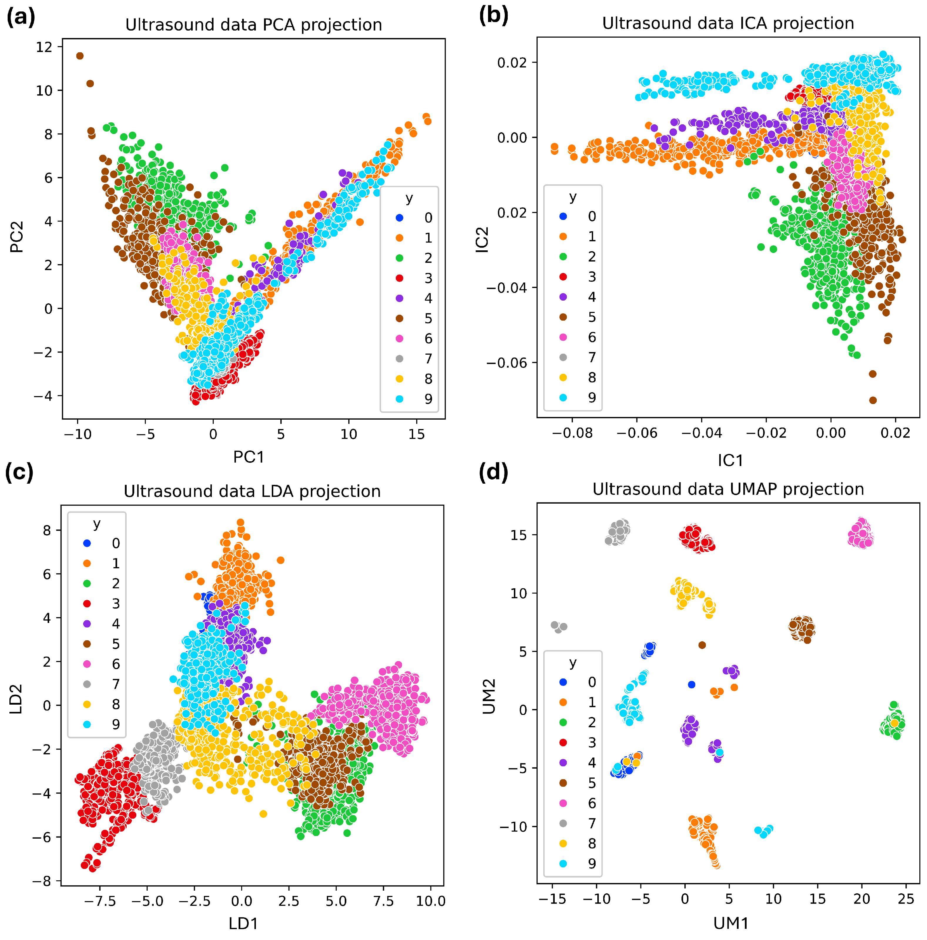
Ultrasonic signals, like many types of real-world data, often exist in high-dimensional spaces and can benefit greatly from dimensionality reduction. This process simplifies the data without losing significant information, making it more manageable and useful for analysis and processing. Dimensionality reduction and feature visualization are crucial for interpreting high-dimensional data. Techniques such as PCA, LDA, ICA, and UMAP offer valuable insights into the data structure by projecting it into two dimensions. PCA captures the most variance by identifying principal components in unlabeled data, making it useful for general data analysis. LDA is tailored for supervised classification, maximizing class separability. ICA excels in identifying statistically independent components, uncovering hidden patterns. UMAP preserves both the local and global data structures, making it effective for visualizing clusters or groups. Figure 6 shows the 2D visualizations of the ultrasonic data using PCA, LDA, ICA, and UMAP, highlighting the distinctions revealed by each method.

The outcomes were evaluated using several algorithms including voting, Logit, GB, AdaBoost, stacking, and bagging. To optimize the hyperparameters of the different classifiers, we employed a systematic method (i.e., grid search). This method involved an exhaustive search over specified parameter values to identify the best combination that enhances the model’s performance. Among the hyperparameters, the “number of estimators” proved to be the most sensitive. Increasing this number generally improve accuracy but also increases the training time. Based on our experiments, we found that using an estimator count of 100 provided a good balance between achieving high accuracy and maintaining a reasonable computation time. In addition, for Logit, regularization strength and the optimization function were selected as 0.9 and ‘lbfgs’, respectively. For voting, the ’hard’ function was used. For GB, the learning rate and depth of regression estimators were selected as 0.1, and 3, respectively. For bagging, the maximum number of samples was selected as 1000. For Adaboost, the learning rate was selected as 1.

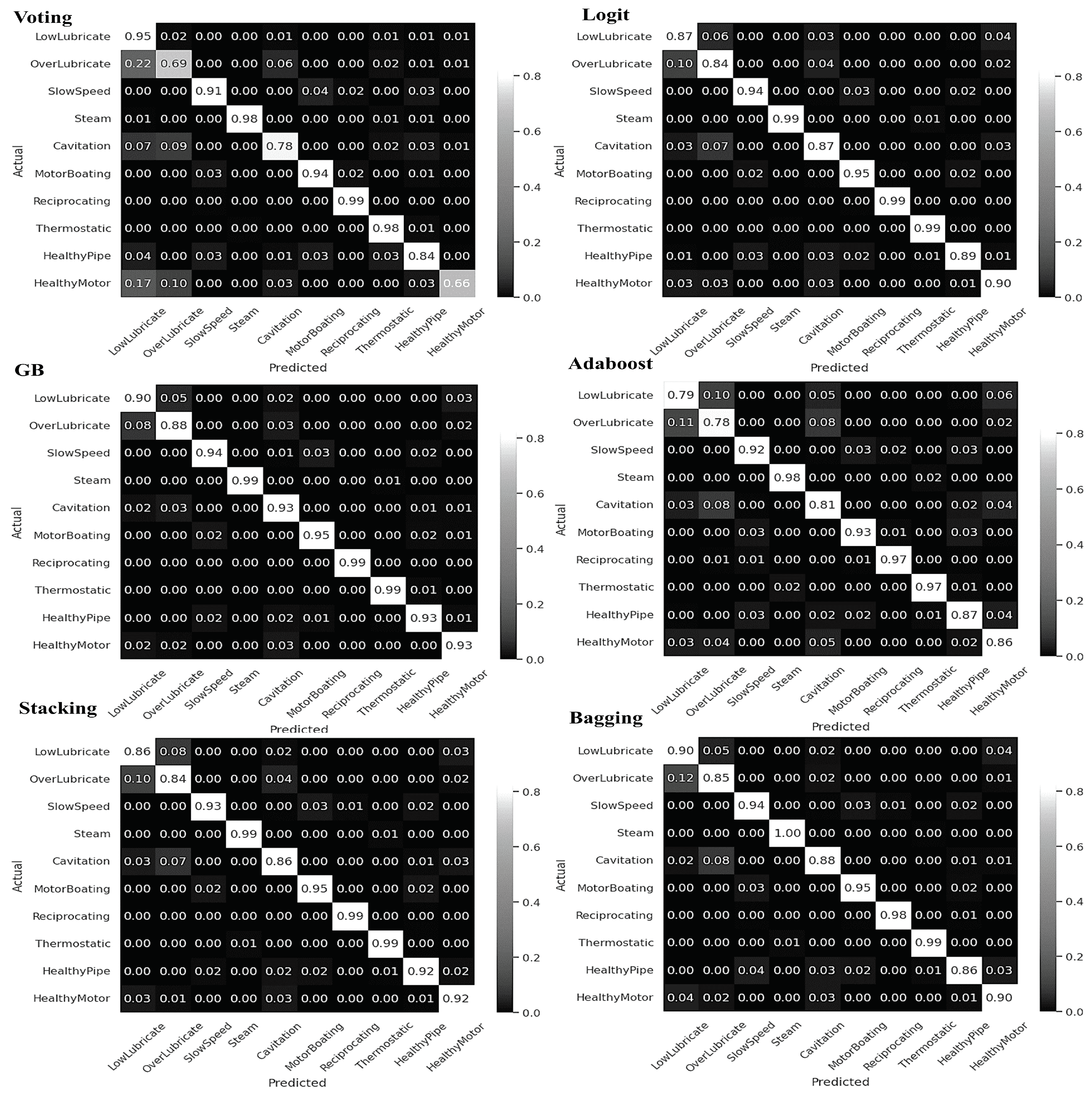
As shown in Figure 7, a confusion matrix was used to assess the classification effectiveness, revealing the notably high accuracy of the GB model. The confusion matrix illustrated the algorithms’ ability to classify various ultrasonic fault states such as low lubrication, over-lubrication, slow speed, steam cavitation, motor boating, reciprocating, thermostatic, healthy pipe, and healthy motor. The main diagonal of the confusion matrix consists of the TP and TN. Higher values on this diagonal indicate better model performance. This tool allowed for quick evaluation of the model’s predictions and highlighted potential areas of error in the ultrasonic dataset.

In addition, in classification tasks, the ROC curve is an important tool for evaluating classifiers. It visually depicts the trade-off between the true positive rate (TPR) and the false positive rate (FPR), helping to determine a classifier’s effectiveness in distinguishing between positive and negative instances. Essentially, a larger area under the ROC curve indicates a higher likelihood of correctly identifying true cases over false ones. As shown in Figure 8, the area under the ROC curve for each category of the dependent variable in GB consistently exceeded 0.99, demonstrating a high level of predictive precision. The ROC curve measures separability, indicating the models’ ability to differentiate among fault classes. It summarizes the trade-off between TPR and FPR for a predictive model across various probability thresholds.

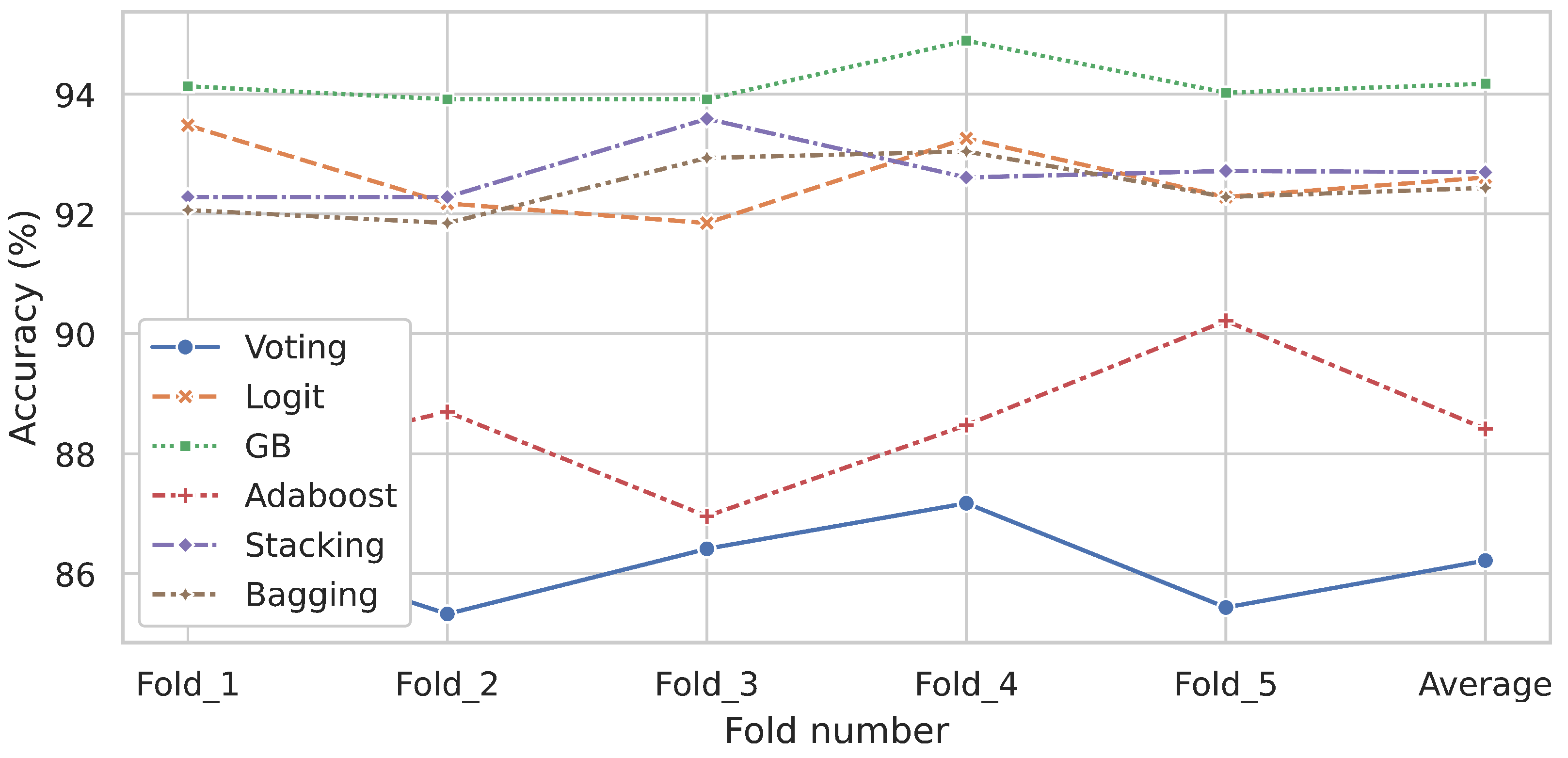
To thoroughly examine and qualitatively evaluate our simulated outcomes across various models, we utilized the k-fold CV technique. This method enabled us to illustrate the differences in classification effectiveness, as shown in Figure 9. It displays the proportion of correct predictions made by each model out of the total number of predictions during 5-fold data splitting. The visual representation helps highlight the comparative strengths and weaknesses of each model, ensuring a comprehensive analysis. Figure 9 also demonstrated that the GB model had a higher proportion of correct predictions compared to the other ensemble methods, indicating its superior efficiency.

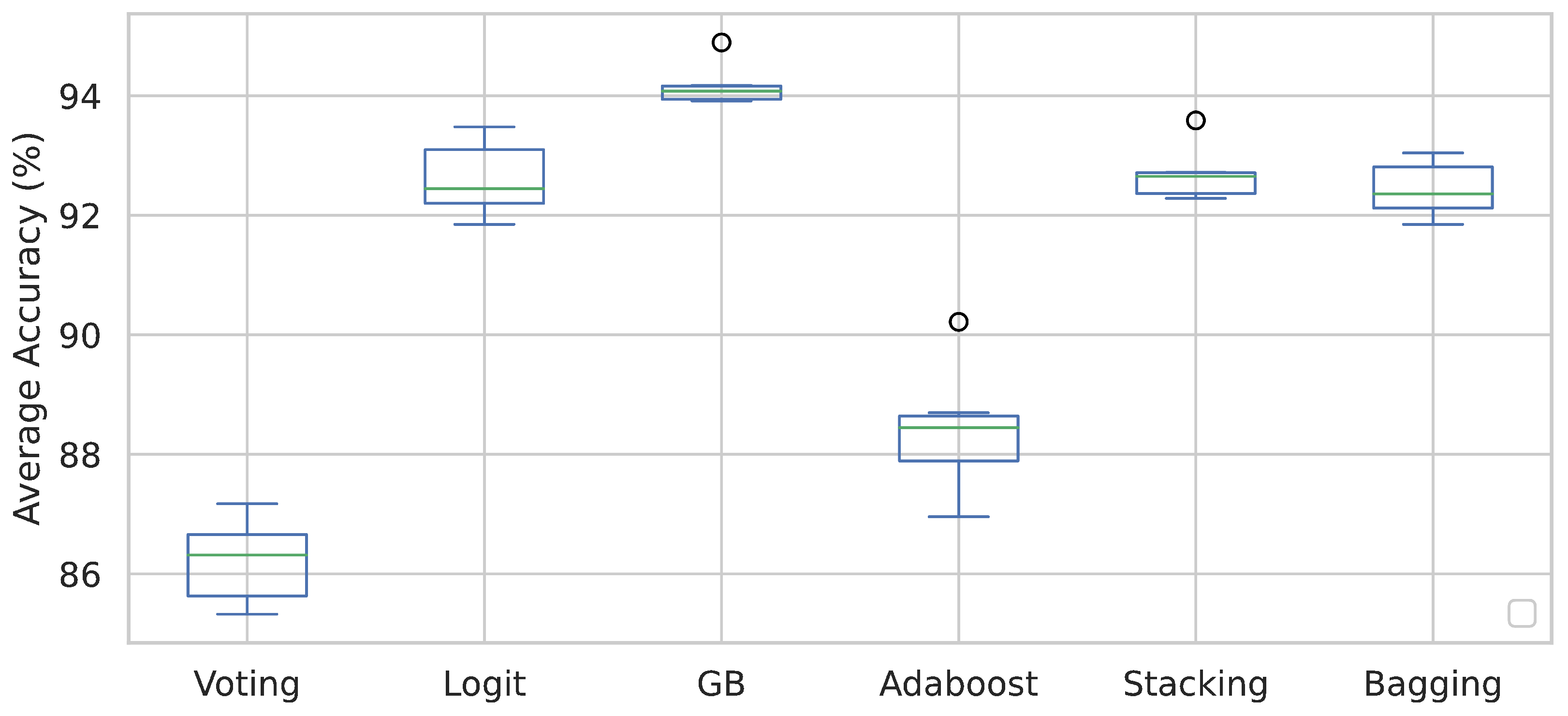
Figure 10 displays a boxplot showing result variations during cross-validation across different folds. This allows for an easy comparison of the accuracy. The boxplot provides a five-number summary: minimum, first quartile, median, third quartile, and maximum. The whiskers extend to depict the rest of the distribution, excluding outliers. As evident, the GB model exhibited the highest accuracy and precision with the lowest distribution range. The stacking classifier indeed showed promising results, ranking second in performance after the GB classifier among the various algorithms tested.

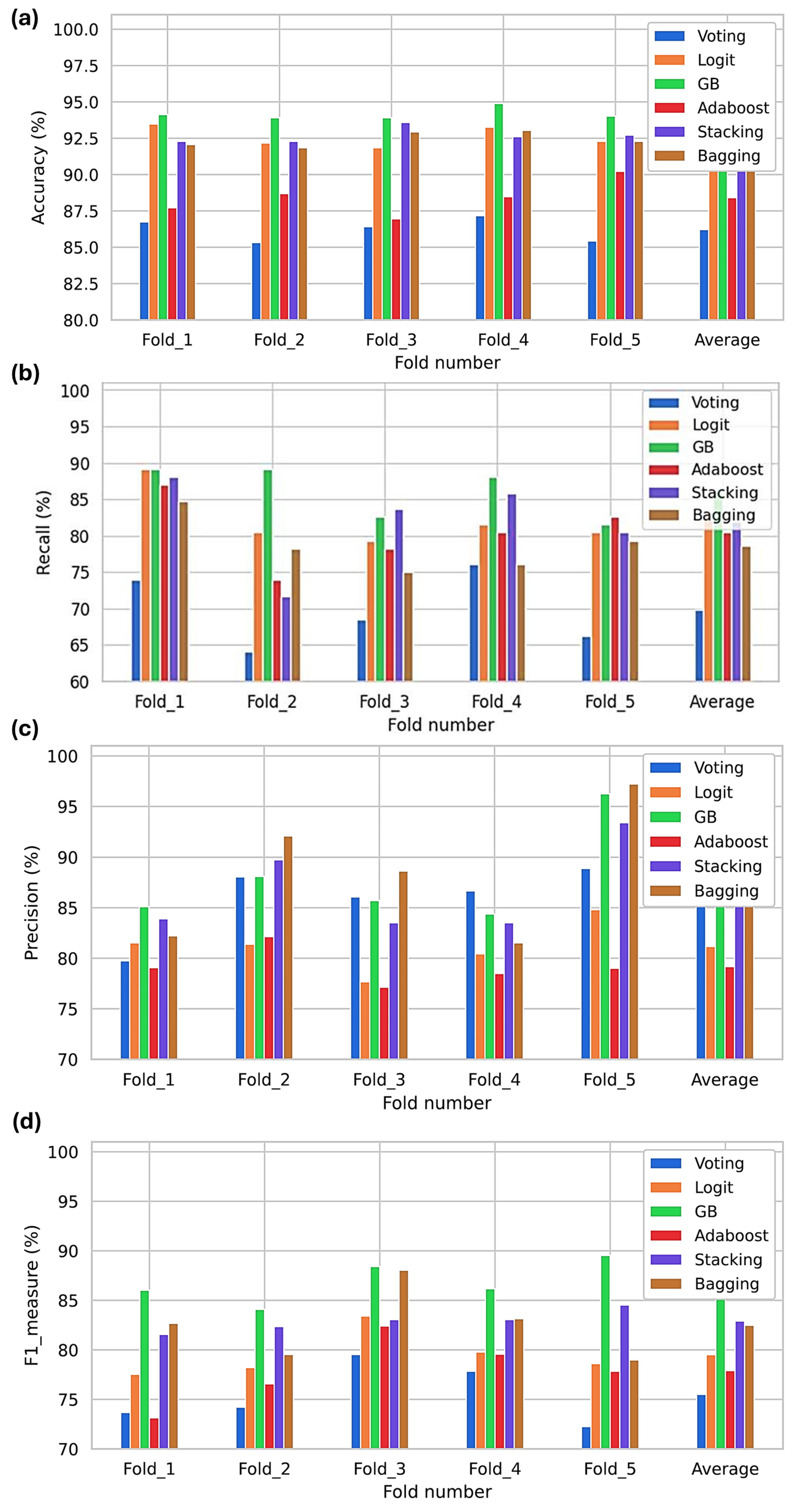
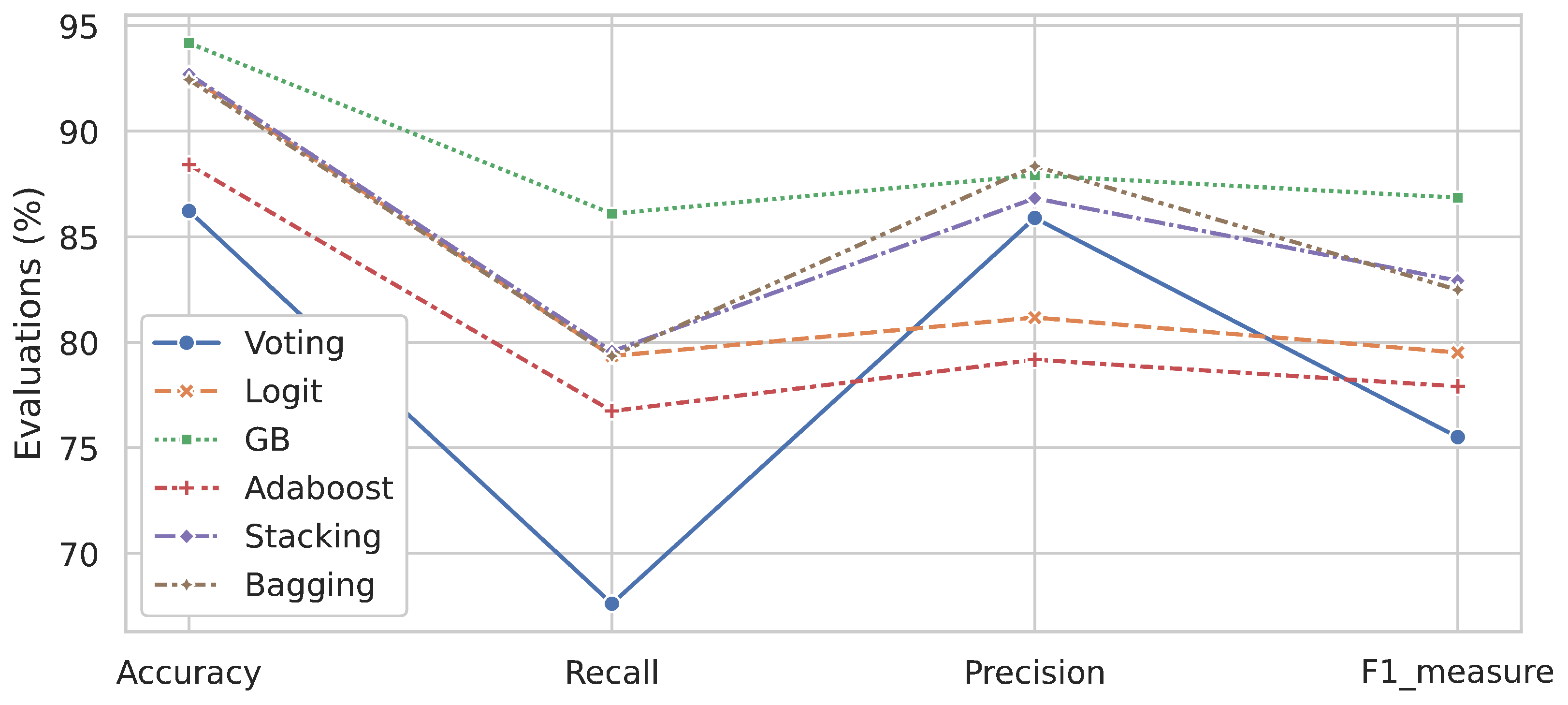
Evaluation metrics of the classifiers are shown as a bar plot in Figure 11 and the overall evaluation results are shown in Figure 12. When focusing solely on the precision metric, the bagging classifier exhibited a marginally superior average than GB. Additionally, the voting classifier demonstrated commendable performance relative to the rest. Upon examining the average evaluation metrics such as accuracy, recall, precision, and F1-measure, it is evident that the GB model surpassed the other classifiers in overall performance. Among the classifiers, the GB algorithm’s average accuracy (94.2%) was about 2% higher, average recall (86.5%) was about 6% higher, and average F1-measure (87.2%) was about 4% higher than the stacking classifier.

GB iteratively builds an ensemble of trees, effectively capturing complex data patterns, handling noise, and dynamically weighing features. In comparison, Adaboost struggles with noisy data and outliers, while bagging, although reducing variance, fails to capture intricate patterns as effectively. Voting aggregates multiple models but falls short when individual models differ significantly in performance, and stacking’s reliance on a strong meta-classifier cannot surpass GB’s individual strength. Logistic regression, being a linear model, cannot handle the non-linear complexities of ultrasonic data, making GB’s non-linear approach superior [29].

To further explore the effectiveness of dimensionality reduction techniques, we incorporated them as input features for the GB model. As mentioned before, the methods we examined included PCA, LDA, ICA, and UMAP. For a comprehensive understanding,

Table 2. Accuracy of the GB model using various dimensionality reduction techniques including PCA, LDA, ICA, and UMAP.

	PCA	LDA	ICA	UMAP
Fold_1	0.802173	0.872826	0.905434	0.726086
Fold_2	0.810869	0.891304	0.929347	0.735869
Fold_3	0.803261	0.875435	0.898913	0.727173
Fold_4	0.797826	0.859782	0.905434	0.713043
Fold_5	0.822826	0.885869	0.928267	0.759782
Average	0.807391	0.876956	0.913478	0.732391

,

Table 3. Recall of the GB model using various dimensionality reduction techniques including PCA, LDA, ICA, and UMAP.

	PCA	LDA	ICA	UMAP
Fold_1	0.739130	0.543478	0.815217	0.528541
Fold_2	0.760869	0.663043	0.793478	0.489130
Fold_3	0.771739	0.543478	0.641304	0.467391
Fold_4	0.752961	0.597826	0.771739	0.576086
Fold_5	0.739130	0.608695	0.758061	0.535028
Average	0.752173	0.591304	0.754347	0.506521

,

Table 4. Precision of the GB model using various dimensionality reduction techniques including PCA, LDA, ICA, and UMAP.

	PCA	LDA	ICA	UMAP
Fold_1	0.704225	0.809523	0.824175	0.511728
Fold_2	0.685393	0.843373	0.935897	0.584415
Fold_3	0.746268	0.788306	0.880597	0.632352
Fold_4	0.647058	0.741935	0.835294	0.638554
Fold_5	0.643678	0.809523	0.851851	0.547619
Average	0.685324	0.798649	0.865563	0.582810

and

Table 5. F1-measure of the GB model using various dimensionality reduction techniques including PCA, LDA, ICA, and UMAP.

	PCA	LDA	ICA	UMAP
Fold_1	0.613496	0.772727	0.819672	0.505494
Fold_2	0.674033	0.872065	0.858823	0.532544
Fold_3	0.628930	0.780219	0.742138	0.537514
Fold_4	0.621468	0.745945	0.802259	0.605714
Fold_5	0.625698	0.772803	0.797687	0.522717
Average	0.632725	0.774324	0.804116	0.540796

provide an in-depth presentation of the respective results, including accuracy, recall, precision, and F1-measure metrics. The experimental data indicate that ICA was superior to the alternative dimensionality methods in terms of performance when used with the GB model.

According to the results depicted in the tables, ICA outperformed the other methods in terms of enhancing the GB model’s accuracy. The high performance of the GB classifier with ICA suggests that this combination expertly captured the underlying structure of the ultrasonic signals.

Implementation

 

Deploying the model on an MCU enables real-time fault detection, reducing the need for manual inspections and minimizing downtime. In this section, two approaches for MCU deployment are investigated: direct classification based on calculated features, and an alternative approach utilizing a dimensionality reduction method as the input to the classifier, as illustrated in Figure 13.

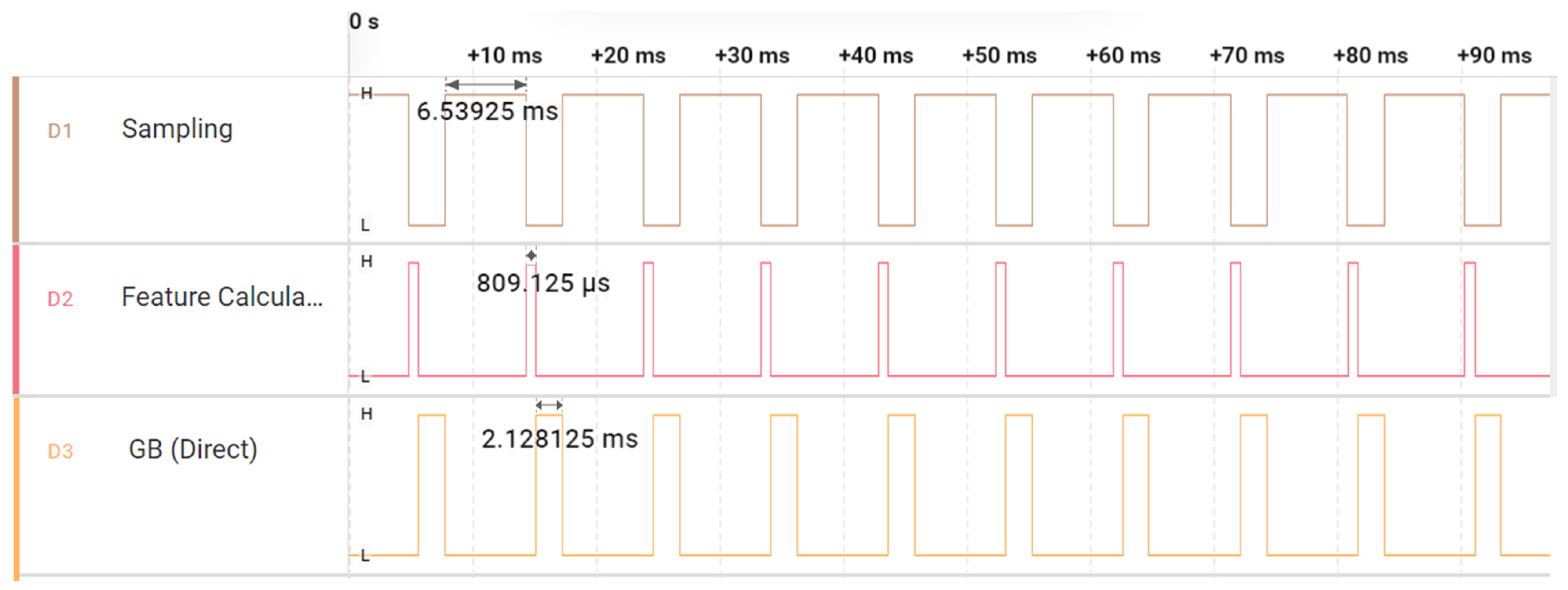
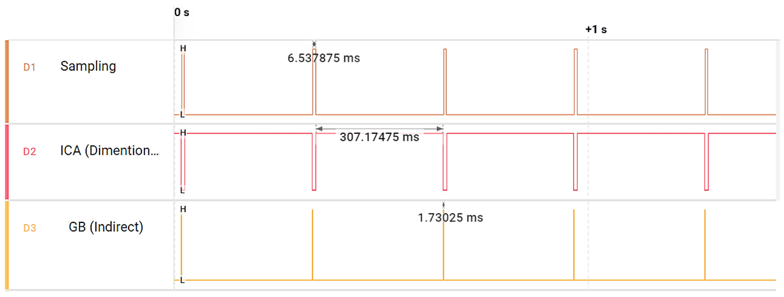
The ICA method exhibiting a higher accuracy (based on Table 2, Table 3, Table 4 and Table 5) was selected for implementation of the second approach. ICA was computed using the FastICA function and then the ’components’ and ’mixing’ matrices were extracted and converted to C array format using the skit-learn library in Python. The models were deployed on a 64 MHz ARM Cortex-M4F MCU. An LA104 Logic Analyzer with 4 channels and a sampling rate of up to 100 MSa/s along with Saleae Logic software were employed for the timing measurements. The first approach, with feature computation on the MCU, took 9.48 ms, while the second approach, with ICA computation on the MCU, took 315.44 ms. Both included 6.54 ms for data sampling and differed in their computation and prediction times, as shown in Figure 14 and Figure 15. The first method was faster with a higher accuracy (94.2% compared to the second method with 91.35%) for our dataset, but the second method had more adaptability for diverse types of data due to the use of the ICA dimensionality reduction model. The choice of approach can vary based on the user’s criteria. Additionally, using ICA before the GB model can lead to better noise reduction and feature extraction, improving the robustness of the classifier in varying conditions. This also enhances the interpretability of the model by separating independent sources within the data, potentially revealing hidden structures in the data and improving the performance of the classifier on new, unseen data by reducing overfitting.

4. Conclusions

This paper presented a comprehensive model for ultrasonic industrial fault detection, targeting diverse applications such as bearings and pipelines using contact sensors. The model’s capability to evaluate and monitor the health of industrial equipment was assessed by detecting and classifying ten different ultrasonic signal conditions. Various dimensionality reduction techniques, including PCA, LDA, ICA, and UMAP, were explored, with ICA being selected for its superior performance. Ensemble classifiers such as voting, logistic regression, gradient boosting, Adaboost, stacking, and bagging were tested, demonstrating the effectiveness of the GB classifier based on performance metrics, confusion matrix, and ROC curves.

The k-fold CV technique was employed to rigorously evaluate the models’ performance, ensuring robustness and generalizability. Experimental results confirmed that the GB classifier outperformed the other models in terms of accuracy, precision, recall, and F1-measure. Our results suggest that using ICA for dimensionality reduction can improve model robustness for different faults.

Advanced techniques like filtering, scaling, dimensionality reductions, and k-fold CV for ensuring evaluation can improve the signal quality for automatic defect recognition, reducing the reliance on skilled operators. Additionally, a data augmentation method is used, which helps improve the model’s ability to generalize and perform well on unseen data.

Furthermore, the model’s real-time applicability was demonstrated through deployment on an ARM Cortex-M4F MCU, showcasing its potential for practical industrial applications. In our study, we explored two approaches: The direct classification method proved to be quicker and more precise, whereas the ICA-based method offered greater adaptability due to its signal-dependent nature and independence from specific features. Based on the results, integrating ultrasonic signal processing with ensemble machine learning techniques improves the efficiency of industrial fault diagnosis. This study not only provides a robust framework for fault detection but also emphasizes the importance of dimensionality reduction and real-time deployment in industrial settings. However, the ICA computation time on the MCU was significantly longer than direct classification, and the dataset could be expanded for better generalizability. The focus on bearings and pipelines limited the scope of the study. Future work could expand to a greater diversity of industrial data classes, explore further optimization of MCU deployment for faster processing times, as well as developing an optimized PCB board and integrating with IoT for comprehensive fault monitoring management.

References

1. Soomro, A.A.; Mokhtar, A.A.; Kurnia, J.C.; Lashari, N.; Lu, H.; Sambo, C. Integrity Assessment of Corroded Oil and Gas Pipelines Using Machine Learning: A Systematic Review. Eng. Fail. Anal. 2022, 131, 105810. [Google Scholar] [CrossRef]
2. Yang, J.; Li, S.; Wang, Z.; Dong, H.; Wang, J.; Tang, S. Using Deep Learning to Detect Defects in Manufacturing: A Comprehensive Survey and Current Challenges. Materials 2020, 13, 5755. [Google Scholar] [CrossRef] [PubMed]
3. Datta, S.; Sarkar, S. A review on different pipeline fault detection methods. J. Loss Prev. Process Ind. 2016, 41, 97–106. [Google Scholar] [CrossRef]
4. Becker, V.; Schwamm, T.; Urschel, S.; Antonino-Daviu, J. Fault detection of circulation pumps on the basis of motor current evaluation. IEEE Trans. Ind. Appl. 2021, 57, 4617–4624. [Google Scholar] [CrossRef]
5. Al-Sabaeei, A.M.; Alhussian, H.; Abdulkadir, S.J.; Jagadeesh, A. Prediction of Oil and Gas Pipeline Failures through Machine Learning Approaches: A Systematic Review. Energy Rep. 2023, 10, 1313–1338. [Google Scholar] [CrossRef]
6. Yu, Y.; Safari, A.; Niu, X.; Drinkwater, B.; Horoshenkov, K.V. Acoustic and Ultrasonic Techniques for Defect Detection and Condition Monitoring in Water and Sewerage Pipes: A Review. Appl. Acoust. 2021, 183, 108282. [Google Scholar] [CrossRef]
7. Salunkhe, V.G.; Khot, S.M.; Desavale, R.G.; Yelve, N.P. Unbalance Bearing Fault Identification Using Highly Accurate Hilbert-Huang Transform Approach. J. Nondestruct. Eval. Diagn. Progn. Eng. Syst. 2023, 6, 031005. [Google Scholar] [CrossRef]
8. Zhang, M.; Guo, Y.; Xie, Q.; Zhang, Y.; Wang, D.; Chen, J. Defect Identification for Oil and Gas Pipeline Safety Based on Autonomous Deep Learning Network. Comput. Commun. 2022, 195, 14–26. [Google Scholar] [CrossRef]
9. Sharma, A. Fault Diagnosis of Bearings Using Recurrences and Artificial Intelligence Techniques. J. Nondestruct. Eval. Diagn. Progn. Eng. Syst. 2022, 5, 031004. [Google Scholar] [CrossRef]
10. Moshrefi, A.; Gratuze, M.; Tawfik, H.H.; Elsayed, M.Y.; Nabki, F. Ensemble AI fault diagnosis model using ultrasonic microphone. In Proceedings of the 2023 IEEE International Ultrasonics Symposium (IUS), Montreal, QC, Canada, 3–8 September 2023; pp. 1–3. [Google Scholar]
11. Shinde, P.V.; Desavale, R.G. Application of Dimension Analysis and Soft Competitive Tool to Predict Compound Faults Present in Rotor-Bearing Systems. Measurement 2022, 193, 110984. [Google Scholar] [CrossRef]
12. Carrera-Avendaño, E.; Urquiza-Beltrán, G.; Trutié-Carrero, E.; Nieto-Jalil, J.M.; Carrillo-Pereyra, C.; Seuret-Jiménez, D. Detection of Crankshaft Faults by Means of a Modified Welch-Bartlett Periodogram. Eng. Fail. Anal. 2022, 132, 105938. [Google Scholar] [CrossRef]
13. Lin, H.C.; Ye, Y.C. Reviews of Bearing Vibration Measurement Using Fast Fourier Transform and Enhanced Fast Fourier Transform Algorithms. Adv. Mech. Eng. 2019, 11, 1687814018816751. [Google Scholar] [CrossRef]
14. Vishwendra, M.A.; Salunkhe, P.S.; Patil, S.V.; Shinde, S.A.; Shinde, P.V.; Desavale, R.G.; Jadhav, P.M.; Dharwadkar, N.V. A Novel Method to Classify Rolling Element Bearing Faults Using K-Nearest Neighbor Machine Learning Algorithm. ASCE-ASME J. Risk Uncertain. Eng. Syst. Part B Mech. Eng. 2022, 8, 031202. [Google Scholar] [CrossRef]
15. Patil, S.M.; Malagi, R.R.; Desavale, R.G.; Sawant, S.H. Fault Identification in a Nonlinear Rotating System Using Dimensional Analysis (DA) and Central Composite Rotatable Design (CCRD). Measurement 2022, 200, 111610. [Google Scholar] [CrossRef]
16. Yuan, J.; Mao, W.; Hu, C.; Zheng, J.; Zheng, D.; Yang, Y. Leak Detection and Localization Techniques in Oil and Gas Pipeline: A Bibliometric and Systematic Review. Eng. Fail. Anal. 2023, 146, 107060. [Google Scholar] [CrossRef]
17. Korlapati, N.V.S.; Khan, F.; Noor, Q.; Mirza, S.; Vaddiraju, S. Review and Analysis of Pipeline Leak Detection Methods. J. Pipeline Sci. Eng. 2022, 2, 100074. [Google Scholar] [CrossRef]
18. Rai, A.; Kim, J.M. A Novel Pipeline Leak Detection Approach Independent of Prior Failure Information. Measurement 2021, 167, 108284. [Google Scholar] [CrossRef]
19. Wang, H.; Fan, Z.; Chen, X.; Cheng, J.; Chen, W.; Wang, Z.; Bu, Y. Automated Classification of Pipeline Defects from Ultrasonic Phased Array Total Focusing Method Imaging. Energy 2022, 5, 8272. [Google Scholar] [CrossRef]
20. Moshrefi, A.; Tawfik, H.H.; Elsayed, M.Y.; Nabki, F. Industrial fault detection employing meta ensemble model based on contact sensor ultrasonic signal. Sensors 2024, 24, 2297. [Google Scholar] [CrossRef] [PubMed]
21. Raišutis, R.; Tumšys, O.; Žukauskas, E.; Samaitis, V.; Draudvilienė, L.; Jankauskas, A. An Inspection Technique for Steel Pipes Wall Condition Using Ultrasonic Guided Helical Waves and a Limited Number of Transducers. Materials 2023, 16, 5410. [Google Scholar] [CrossRef]
22. Norli, P.; Frijlink, M.; Standal, Ø.K.-V.; Bjåstad, T.G.; Prieur, F.; Vallée, E. Ultrasonic Detection of Stress Corrosion Cracks in Pipe Samples Using Guided Waves. In Proceedings of the 2018 IEEE International Ultrasonics Symposium (IUS), Kobe, Japan, 22–25 October 2018; pp. 1–4. [Google Scholar] [CrossRef]
23. Wei, M.; Miao, Q.; Jiang, L. Feature Extraction Method for Ultrasonic Pipeline Defects Based on Fractional-Order VMD. Nondestruct. Test. Eval. 2024, 39, 1–20. [Google Scholar] [CrossRef]
24. Cai, L.; Diao, Z.; Chen, F.; Guan, L.; Xu, G. Identification method of circumferential declination based on amplitude reduction of pipeline ultrasonic internal inspection signals. Nondestruct. Test. Eval. 2024, 37, 1–17. [Google Scholar] [CrossRef]
25. Yadavendra, S. A comparative study of breast cancer tumor classification by classical machine learning methods and deep learning method. Mach. Vis. Appl. 2020, 31, 46. [Google Scholar] [CrossRef]
26. Dong, X.; Yu, Z.; Cao, W.; Shi, Y.; Ma, Q. A survey on ensemble learning. Front. Comput. Sci. 2020, 14, 241–258. [Google Scholar] [CrossRef]
27. Tanha, J.; Abdi, Y.; Samadi, N.; Razzaghi, N.; Asadpour, M. Boosting Methods for Multi-Class Imbalanced Data Classification: An Experimental Review. J. Big Data 2020, 7, 1–47. [Google Scholar] [CrossRef]
28. Ju, X.; Salibián-Barrera, M. Robust boosting for regression problems. Comput. Stat. Data Anal. 2021, 153, 107065. [Google Scholar] [CrossRef]
29. González, S.; García, S.; Del Ser, J.; Rokach, L.; Herrera, F. A Practical Tutorial on Bagging and Boosting Based Ensembles for Machine Learning: Algorithms, Software Tools, Performance Study, Practical Perspectives, and Opportunities. Inf. Fusion 2020, 64, 205–237. [Google Scholar] [CrossRef]
30. Mohapatra, S.; Maneesha, S.; Patra, P.K.; Mohanty, S. Heart Diseases Prediction Based on Stacking Classifiers Model. Procedia Comput. Sci. 2023, 218, 1621–1630. [Google Scholar] [CrossRef]
31. Nti, I.K.; Nyarko-Boateng, O.; Aning, J. Performance of Machine Learning Algorithms with Different K Values in K-Fold Cross-Validation. Int. J. Inf. Technol. Comput. Sci. 2021, 13, 61–71. [Google Scholar] [CrossRef]
32. Marcot, B.G.; Hanea, A.M. What Is an Optimal Value of K in K-Fold Cross-Validation in Discrete Bayesian Network Analysis? Comput. Stat. 2021, 36, 2009–2031. [Google Scholar] [CrossRef]
33. Yadav, S.; Shukla, S. Analysis of K-Fold Cross-Validation over Hold-Out Validation on Colossal Datasets for Quality Classification. In Proceedings of the 2016 IEEE 6th International Conference on Advanced Computing (IACC), Bhimavaram, India, 27–28 February 2016; pp. 78–83. [Google Scholar] [CrossRef]
34. Jia, W.; Sun, M.; Lian, J.; Hou, S. Feature dimensionality reduction: A review. Complex Intell. Syst. 2022, 8, 2663–2693. [Google Scholar] [CrossRef]
35. Toma, R.N.; Kim, J.M. Bearing Fault Classification of Induction Motor Using Statistical Features and Machine Learning Algorithms. Lect. Notes Netw. Syst. 2022, 418, 243–254. [Google Scholar] [CrossRef]
36. Kurita, T. Principal Component Analysis (PCA). Comput. Vis. A Ref. Guid. 2019, 19, 303–342. [Google Scholar]
37. McConn, J.L.; Lamoureux, C.R.; Poudel, S.; Palsson, B.O.; Sastry, A.V. Optimal dimensionality selection for independent component analysis of transcriptomic data. BMC Bioinform. 2021, 22, 584. [Google Scholar] [CrossRef] [PubMed]
38. McInnes, L.; Healy, J.; Melville, J. UMAP: Uniform Manifold Approximation and Projection for Dimension Reduction. arXiv 2018, arXiv:1802.03426. [Google Scholar]
39. Tharwat, A.; Gaber, T.; Ibrahim, A.; Hassanien, A.E. Linear Discriminant Analysis: A Detailed Tutorial. AI Commun. 2017, 30, 169–190. [Google Scholar] [CrossRef]
40. Sravani, S.; Karthikeyan, P.R. Detection of cardiovascular disease using KNN in comparison with naive bayes to measure precision, recall, and f-score. In AIP Conference Proceedings; AIP Publishing: New York, NY, USA, 2023; Volume 2821. [Google Scholar]
41. UE Systems Co. Available online: https://www.uesystems.com/resources/sound-library/ (accessed on 1 January 2020).
Figure 1. Study workflow diagram for ultrasonic fault diagnosis.
Applsci 14 06397 g001
Figure 2. Boosting algorithm.
Applsci 14 06397 g002
Figure 3. Bagging algorithm.
Applsci 14 06397 g003
Figure 4. Stacking algorithm.
Applsci 14 06397 g004
Figure 5. k-fold CV algorithm structure to evaluate the ultrasonic diagnosis.
Applsci 14 06397 g005
Figure 6. Two-dimensional representations of the ultrasonic data for the different dimensionality reduction methods evaluated: (a) PCA, (b) ICA (c) LDA, and (d) UMAP.
Applsci 14 06397 g006
Figure 7. Confusion matrix for different ensemble classifiers including the voting, Logit, GB, Adaboost, stacking, and bagging algorithms.
Applsci 14 06397 g007
Figure 8. ROC curves for the voting, Logit, GB, Adaboost, stacking, and bagging algorithms.
Applsci 14 06397 g008
Figure 9. Accuracy analysis of the models using k-fold CV.
Applsci 14 06397 g009
Figure 10. Boxplot of the accuracies for the six classifiers.
Applsci 14 06397 g010
Figure 11. Barplot of 5-fold CV for different ensemble classifiers based on the (a) accuracy, (b) recall, (c) precision, and (d) F1 measure.
Applsci 14 06397 g011
Figure 12. Evaluation results for the four metrics including accuracy, recall, precision, and F1-measure for different ensemble classifiers.
Applsci 14 06397 g012
Figure 13. Diagram of the two deployed approaches.
Applsci 14 06397 g013
Figure 14. Execution time for the first approach deployed —direct classification.
Applsci 14 06397 g014
Figure 15. Execution time for the second deployed approach—ICA dimensionality reduction prior to classification.
Applsci 14 06397 g015