Abstract
At present, the optimization of public transportation networks and vehicle scheduling are carried out independently in stages. However, through analysis, it has been found that scheduling information such as route schedules is an important factor related to passenger route selection. Therefore, in order to further improve the optimization effect, this article proposes an innovative idea of simultaneously optimizing the line network and scheduling. Based on the construction of a real–virtual public transportation network, this article constructs a synchronous optimization model for the line network and scheduling by considering both passenger waiting and on-board time. To achieve the consideration of passengers for different route choices, a shortest path traversal algorithm based on Yen was proposed to analyze the number and weight of the shortest paths between the same OD, and a genetic algorithm was used to solve the model. Finally, the effectiveness of the model was verified through numerical examples, and the results showed that synchronous optimization was superior to phased optimization: the passenger time cost was reduced by 21.5%, the bus operation cost was reduced by 13.7%, and the total bus system cost was reduced by 18.0%.
1. Introduction
With the acceleration of urbanization and rapid economic development in our country, the number of motor vehicles and the travel demands of residents are also rapidly increasing. Traffic congestion has become common and is becoming increasingly severe.
To alleviate the current pressure on transportation, our country is vigorously promoting the development of public transportation, especially in large cities where public transportation is developing rapidly. For example, in Shenzhen, the length of operational rail transit lines exceeded 400 km in 2020, reaching 422.6 km, a year-on-year increase of 33.9%. The length of bus operating routes reached 21,310.53 km, a year-on-year decrease of 1.4%. Currently, in major cities across the country, transportation modes such as buses, subways, taxis, and trams together form a public transportation network, with overall passenger flow continually increasing. In 2019, the average daily passenger flow of public transportation in Shenzhen was 11.06 million passengers per day, an increase of 2.65 million passengers per day compared to 2011. In 2020, due to the impact of the COVID-19 pandemic, the average daily passenger volume for the entire year was 8.226 million passengers, a year-on-year decrease of 25.6%. As the pandemic situation improved and new subway lines opened, public transportation passenger flow in December rose to the highest level of the year, with an average daily passenger volume of 10.603 million passengers, recovering to 94.1% of the same period in 2019.
To improve the transportation efficiency of buses and balance the supply and demand of the bus system, it is necessary to replan and redesign the bus network. This will help avoid significant overlap with rail transit lines, preventing redundant routes and resource waste. At the same time, it is crucial to ensure seamless connections and transfers between buses and rail transit, thereby meeting passengers’ travel needs and reducing travel costs.
After conducting domestic and international research and analysis on bus networks, it was found that existing studies overlook the impact of scheduling on bus network optimization. They also fail to consider passengers’ waiting costs when calculating the total travel costs for passengers. Analysis of passenger card swiping data revealed a moderate correlation between passengers’ route choices and the frequency of bus services. Therefore, this paper includes scheduling considerations in the optimization of bus networks.
Scholars both domestically and internationally have conducted relatively mature research on the optimization of urban bus networks. The majority of research on network optimization focuses on three aspects: theory, model construction, and algorithm development.
Theoretical Methods: Pu Han et al. proposed a bus network optimization method based on multilayer complex networks [1]. Mitra Subhro et al. presented a multi-objective bus network optimization method [2]. Petit Antoine et al. introduced a bus network design method based on aggregate networks and continuous approximation models [3]. Szeto et al. proposed a network optimization method for urban transportation networks and road networks [4]. Zhang L developed a public transportation route network (PTRN) auxiliary optimization method based on link prediction [5]. Klier MJ introduced a novel optimization method for designing public transportation networks, maximizing the expected total number of public transportation passengers under budget constraints [6]. Yin J studied the coordinated train timetable optimization of urban rail transit networks and proposed a mathematical formula to generate the best-coordinated train timetable synchronously [7]. Liang M established a multi-objective model based on two conflicting objectives, and developed two populations to simultaneously optimize the network and frequency [8]. Wang C introduced a multi-level multi-mode network design method [9]. Huang A studied a demand-responsive public transit (DRT) service that adjusts paths continuously based on dynamic passenger demands, maximizing system efficiency while considering passengers’ preferred time windows [10]. Gong M proposed designing a modularized fleet-based CB network based on transfers, optimizing passenger route assignments simultaneously [11]. Yang J proposed a novel initial route set generation algorithm and a route set size alternating heuristic algorithm embedded in a solution framework based on non-dominated sorting genetic algorithm-II (NSGA-II) to generate approximate Pareto frontiers [12]. Yao E presented a new method (MVT-E-VSP) for scheduling electric vehicles of multiple types [13]. Guo R optimized the operational performance of a bilateral BRT with elastic demand, minimizing the generalized time costs per passenger [14]. Li Wenyong et al. proposed a microcirculation bus network planning method based on hierarchical clustering [15]. Shi Xiaowei et al. proposed a rail transit feeder bus network optimization method based on the shortest route labeling model [16]. Huang Min et al. proposed a method for constructing different levels of bus routes and optimizing them separately according to different levels and functions [17]. Yight F et al. provided a hybrid approach to optimize the theoretical method for sequence-dependent pipeline scheduling problems [18].
Model Construction: Ren Hualing et al. proposed a new bus allocation model based on line and node strategies [19]. Shi Qingshuai et al. proposed a public transportation route optimization evaluation model based on multi-source bus data [20]. Fan W introduced a heuristic method based on Tabu Search (TS) and applied it to public transportation network design with variable demand [21]. Huang D developed a new optimization model for demand-responsive customized bus (CB) network design, including dynamic and static phases [22]. Li X proposed a joint optimization model for conventional charging electric bus network scheduling and fixed charger deployment considering partial charging policies and time-of-use electricity prices [23]. Steiner K developed a strategic network planning optimization model for bus routes [24]. Chai S established a multi-objective bus network design model that not only considers transfer impacts but also takes into account delays in passenger travel time due to congestion [25]. Wei M presented a mathematical model for designing feeder bus services to improve the service quality and accessibility of transportation hubs [26].
Algorithm Development: Z. Tang et al. proposed coupling local deterministic search and global evolutionary algorithms for bus network optimization [27]. Kuan et al. conducted research on bus network optimization using a combination of genetic algorithms and ant colony algorithms [28]. Ngamchai et al. introduced a method that combines various genetic operation mechanisms for bus network optimization design [29]. Bourbonnais PL used precise local road network data and representative public transportation demand data for genetic algorithm optimization to generate reasonable solutions [30]. Ding Jianxun et al. proposed using an improved K-shortest path algorithm for bus network optimization research [31]. Luo Xiaoling et al. proposed using the K-means clustering algorithm to perform cluster analysis on bus stations for network optimization research [32]. Gao Mingyao et al. proposed using an improved Particle Swarm Optimization (PSO) algorithm to solve the bus network optimization model [33]. Xin Yi et al. proposed using the NSGA-II algorithm to solve the multi-objective bus network optimization model [34]. Wang Ning et al. proposed using a cellular genetic algorithm to solve the feeder bus network model [35]. Yu Lijun et al. designed an improved simulated annealing algorithm to optimize and solve the network optimization model [36]. Wu Kexin et al. used an improved ant colony algorithm for network optimization of bus networks [37].
Overall, the optimization research of bus networks has achieved numerous excellent research results in both theoretical methods and model construction as well as algorithm development, providing a theoretical research basis for the optimization design work of this paper’s network. However, these achievements still have some shortcomings in their practical application:
(1) Ignored Passenger Route Selection: Both domestic and international scholars often assume that passengers choose the shortest time or the fewest transfers when optimizing bus networks. However, when multiple paths between the same origin–destination (OD) stations meet the passengers’ criteria, passengers may selectively choose different routes to travel.
(2) Did Not Consider the Impact of Scheduling on Bus Network Optimization: Previous research has often overlooked the influence of route scheduling on passenger route selection during the network layout phase. When calculating the total travel cost for passengers, waiting costs at bus stops were not taken into account. This incomplete consideration in calculating the total time cost for passengers is directly related to vehicle scheduling because passengers’ waiting costs are directly correlated with scheduling.
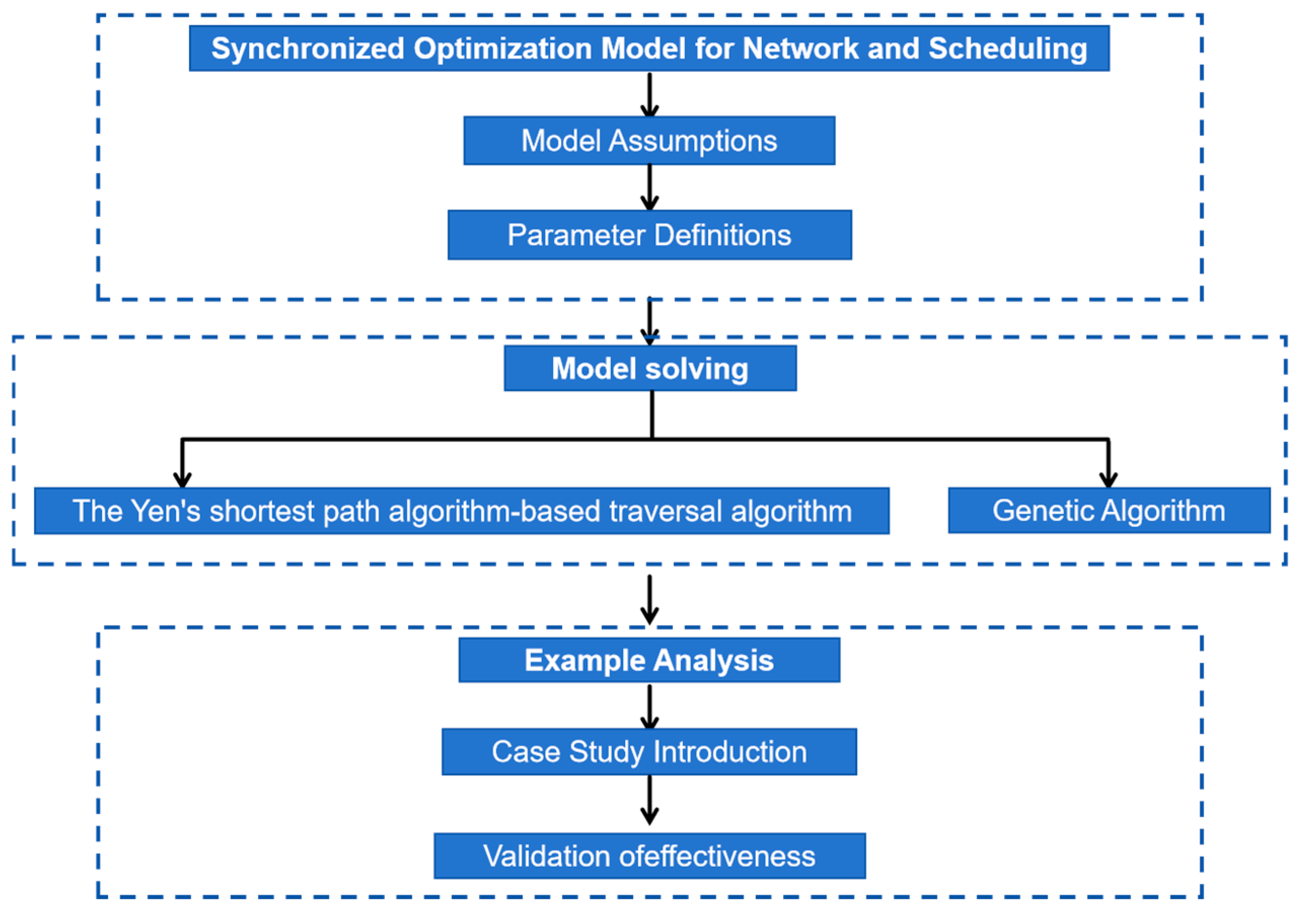
To help readers better understand the structure and content of this paper, the technical roadmap of chapter contents is illustrated in Figure 1. A brief overview of each chapter is provided below:

Figure 1.
Technical roadmap of Section contents.
Section 2 introduces the construction and solution of the integrated optimization model for the bus network and scheduling. It first defines the research scope of the bus network problem in this paper, presents the assumptions for model construction, and then describes the objective function and constraints of the integrated optimization model. Based on the construction of an actual–virtual bus network, which balances the interests of both passengers and operators, the chapter establishes the integrated optimization model.
Section 3 applies Yen’s algorithm to analyze reachable paths between the same origin–destination (OD) pairs. The paths are sorted based on their weights, and the parameter K is flexibly set to accommodate different ODs. Since such problems are typically NP-Hard and involve high computational difficulty and complexity, intelligent optimization algorithms are usually employed. Given the computational complexity of large-scale bus network construction, we chose the efficient genetic algorithm to solve the integrated optimization model.
Section 4 validates the effectiveness of the integrated optimization model for a bus network and scheduling based on the genetic algorithm through specific case studies. By setting weights between stations, the algorithm’s effectiveness in the optimization process was verified. The cases were optimized in stages and synchronously, with results compared between them. Finally, sensitivity analysis was conducted focusing on different stakeholders, confirming the conclusion that cost reduction effects are more significant.
2. Synchronized Optimization Model for Network and Scheduling
2.1. Model Assumptions
Due to the multifaceted nature of factors influencing the bus system, the following assumptions are made to accurately define the bus network optimization problem addressed in this study:
(1) Passengers choose the shortest travel time route to ride; when multiple routes can satisfy the shortest travel time, passengers choose based on the proportion of the total number of trips taken by the vehicles on that OD route. (Shortest Time)
(2) The waiting cost for passengers is assumed to be half of the average waiting time for the selected route, which is equal to half of the departure interval of the vehicles on the chosen route.
(3) The vehicles on each route are assumed to be identical except for the number of trips. Differences in factors such as road traffic, passenger load, and driving speed that may affect passenger route selection are ignored.
(4) The total travel time for passengers includes waiting time, time spent on the vehicle, walking time from the origin to the bus stop, and walking time from the bus stop to the destination.
(5) Passenger transfers are limited to the same bus stop. If there is no direct route between the origin and destination, passengers need to get off at a stop on the initial route and board another bus passing through that stop to reach the destination, only considering transfers at the same stop.
(6) It is assumed that passengers can board the next available vehicle on the desired route after arriving at the stop, without any capacity restrictions on the vehicles.
2.2. Parameter Definitions
: Under the bus network, the shortest travel time required for passengers to travel from Station to Station (s);
: The waiting time for passengers traveling from site to site along their chosen shortest path (s);
: The bus’s stopping time during its journey from site to site (s);
: Passenger’s on-board time from site to site (s);
: The stopping time of a bus during its journey from station to station (s);
: The average dwell time of a bus at a bus stop (s);
: The operational time of route (s);
: Operating costs (s);
: The cost of purchasing a bus (s);
: The operating costs of each bus route (s);
: Cost per unit distance for a bus (s);
: The daily purchase cost per bus (s);
: Bus network;
: Traffic demand from station to station ;
: The number of stops between stations and on the selected route;
: The length of the segment between stations i and j on route r (km);
S: The number of total stations represented;
: The number of stations between stations i and j on route ;
: The minimum length of a bus route (km);
: The maximum length of a bus route (km);
: The minimum departure interval for buses on a bus route;
: Route ‘s bus departure interval;
: The maximum departure interval for buses on a bus route;
: The length of route (km);
: The straight-line distance between the starting and ending points of route (km);
: The weighting coefficient between time cost and operating cost;
: The conversion coefficient between time cost and operating cost;
: The passenger waiting coefficient is due to passengers arriving evenly, and vehicle arrivals follow a Poisson distribution, .5;
: The value is 1 if the shortest path from site to site passes through route r, and 0 if it does not;
: The average speed of a bus (m/s);
: The segment between adjacent stations and on route has a value of 1 when it is on the route r, and a value of 0 when it is not;
: The station in route .
2.3. Model Construction
Consideration of optimizing the design of city bus networks with scheduling aims to minimize passenger time cost and bus operation cost. Constraints include the route length, headway, non-repeating route stations, and non-linear route coefficients. A synchronous optimization model is developed for both the network and scheduling.
2.3.1. The Objective Function
The optimization objective of the bus network should comprehensively consider the interests of both passengers and bus operators. Passengers seek short travel times, while operators aim for efficient resource utilization and minimized investment costs. Therefore, in the optimization design of the bus network and scheduling model in this paper, the interests of both passengers and bus operators are simultaneously considered. The goal is to reduce passenger travel time and lower bus operation costs, aiming to minimize costs for both passengers and bus operators in the bus network.
Passenger Travel Cost
Passenger travel cost mainly refers to the total travel time for passengers within the network, which includes waiting time and in-vehicle time.
(1) Waiting time
In the model assumptions mentioned earlier, it is assumed that passengers, upon arriving at the station, can board the first bus of the target route for travel, meaning passengers can all catch the next scheduled bus of the target route. Therefore, the waiting time for passengers mainly depends on the headway of the route they are waiting for, with passenger waiting time being half of the headway of the selected route. The passenger waiting time is expressed as:
(2) In-vehicle time
In-vehicle time mainly consists of two parts: inter-stop travel time and dwell time at stops. Ignoring the influence of road and other external factors, travel time is related to distance and travel speed, while dwell time is related to the number of intermediate stops. Therefore, travel time and dwell time are represented as follows:
Based on the above, the total time cost for passengers can be expressed as follows:
Bus Operation Cost
The expenses of bus operators mainly include the procurement of buses, construction of stations, wages and salaries of staff, management fees, vehicle insurance, fuel costs, vehicle depreciation expenses, and taxes, among others. In this paper, when considering costs, only the operational costs of buses are taken into account, which are mainly reflected in economic costs. This specifically refers to the vehicle procurement costs and operational costs of each route within the bus network.
(1) Vehicle procurement cost
To minimize vehicle procurement costs and maximize vehicle utilization, it is necessary to reduce the number of vehicles as much as possible. However, it is also important to ensure that there is a bus available at the departure station to meet the next scheduled departure for each route. This requires ensuring that the cumulative headway is greater than the duration of each route, meaning that the minimum number of vehicles required for each route should satisfy the following condition:
Therefore, the minimum vehicle procurement cost is:
(2) Route operation cost
The operational cost of a bus route mainly includes the vehicle’s operating cost, which is primarily related to the frequency of trips and the cost per trip. Therefore, the minimum operational cost of a route is represented as follows:
Therefore, the bus operation cost is represented as follows:
2.3.2. Constraint Conditions
To provide a detailed definition of the conditions set in the model, the following constraints are imposed to further restrict the model:
(1) Route length
In bus network optimization, if bus routes are too short, operational costs increase, while excessively long routes reduce passenger comfort. Therefore, to better meet passenger needs, routes should not be excessively short or long. The length of each route needs to satisfy the following constraint:
(2) Headway
Setting the headway correctly is crucial. Too long a headway increases passenger waiting time, leading to higher passenger time costs. On the other hand, too short a headway results in a higher number of required vehicles, leading to increased operational costs for bus operators. Therefore, the headway needs to satisfy the following constraint:
(3) Non-repeating route stations
In the designed bus network, to avoid bus routes forming loops which increase passenger travel costs and lead to resource waste, a constraint is set that each bus route should contain non-repeating bus stations. This means that each bus station should only appear once along each bus route.
(4) Non-linear coefficient
To avoid excessive detours in the established routes, reduce passenger travel time costs, and improve the quality of bus services, the non-linear coefficient of routes is constrained based on the “Urban Road Traffic Planning and Design Code” in this paper’s synchronous optimization model.
2.3.3. Synchronous Optimization Model for Both Network and Scheduling
Based on the above, the synchronous optimization model for both network and scheduling in this paper is represented as follows:
The objective function in the synchronous optimization model constructed in this paper is divided into two parts: passenger time cost and bus operation cost.
Passenger time cost includes: waiting time (Equation (1)), inter-stop time (Equation (2)), dwell time (Equation (3)); bus operation cost includes: vehicle procurement cost (Equation (6)), route operation cost (Equation (7)).
Constraints include: route length (Equation (9)), headway (Equation (10)), non-repeating route stations (Equation (11)), non-linear coefficient (Equation (12)).
3. Model Solving
The synchronous optimization model proposed in this paper assumes that passengers choose the shortest path when calculating the in-vehicle travel time cost in the objective function. However, there may be multiple shortest paths between the same origin–destination (OD) stations. In such cases, it is essential to consider passengers’ choices among different paths. Therefore, it is necessary to statistically analyze the number of shortest paths between each OD pair. The Yen algorithm can analyze reachable paths between the same OD pair, count these paths based on their weights, and provide a sorted ranking of weights. In this paper, the Yen algorithm is utilized to statistically analyze the shortest paths between different OD pairs. During application, a flexible approach is taken to set the K value (number of shortest paths to consider) by comparing the weights of adjacent shortest paths. This allows for adaptable selection of the K value for different OD stations.
This paper proposes a synchronous optimization model that deals with a combinatorial optimization problem. Such problems have a finite number of combination possibilities, and the optimal solution can be found using an enumeration method. However, when there are many decision variables, the computational complexity of the problem can become extremely large, often exhibiting exponential growth. For example, when considering an optimized bus network with N network sites, n dimensions, r routes, and a headway range of R, the enumeration would require iterations, resulting in a massive computational load. This falls into the category of typical NP-hard problems. Due to the high computational difficulty and complexity of such problems, intelligent optimization algorithms are commonly used for solving them. Considering the characteristics of large-scale bus network construction in this research, which involves a high number of site dimensions and computational complexity, genetic algorithms are chosen as they offer high operational efficiency and are widely applicable for solving large-scale combinatorial optimization and non-linear optimization problems. Therefore, this paper employs a genetic algorithm to solve the synchronous optimization model.
For the synchronous optimization problem of the bus network and scheduling discussed in this paper, relevant algorithm designs have been made for the synchronous optimization model, which are specifically described as follows:
3.1. The Yen’s Shortest Path Algorithm-Based Traversal Algorithm
This paper considers the situation where passengers choose which route to take during their travel. When calculating the total travel cost for passengers between various origin–destination (OD) stations, it is assumed that passengers always choose the shortest path. However, in cases where there are multiple shortest paths between OD pairs, considering passengers’ choices among these paths becomes necessary. Therefore, it is essential to analyze and compute the shortest paths between each OD pair. To address this analytical need, the Yen’s shortest path algorithm is selected to analyze the shortest path scenarios between different OD pairs. The Yen algorithm, proposed by Jin Y. Yen in 1971 for solving the KSP (K-Shortest Paths) problem, is based on the shortest path algorithm and computes the first K-shortest paths between OD stations. It is suitable for calculating the single-source K-shortest paths in directed acyclic graphs with non-negative weighted edges [38]. In this paper, the basic process of the Yen algorithm-based shortest path traversal is as follows:
(1) Given the origin station and destination station , for the initial traversal, set the value of to 1. This will find the first shortest path for the OD pair and the corresponding weight .
(2) When seeking the second shortest path with K set to 2, the process is as follows: ① Update the shortest paths for each segment: Initially, set the weights of all segments on the path to infinity. Calculate the new shortest path for each segment by setting the weights of the segments on the path to infinity in sequence. Concatenate the resulting new shortest paths with the original path. The number of computations is equal to the number of segments in the path. ② Initialize the candidate route set . If the newly obtained paths from the previous step are non-empty and meet the conditions of non-repeating stations and being different from the previously selected path , add them to the candidate route set Remove any duplicates from the candidate route set . ③ Select the shortest route and update the candidate route set . From the non-empty candidate route set , select the path with the minimum weight as the second shortest path , with a weight of Remove this path from the candidate route set . This process ensures that the second shortest path is found while considering non-repeating stations and avoiding duplication with the first selected path .
(3) When finding the -th shortest path with K set to , the process is as follows: ① Update the shortest paths for each segment: Start by setting the weights of all segments on the path to infinity. Calculate the new shortest path for each segment by setting the weights of the segments on the path to infinity in sequence. Concatenate the resulting new shortest paths with the original path. The number of computations is equal to the number of segments in the path. ② Initialize the candidate route set If the newly obtained paths from the previous step are non-empty and meet the conditions of non-repeating stations and being different from the previously selected paths to , add them to the candidate route set Remove any duplicates from the candidate route set . ③ Select the shortest route and update the candidate route set . From the non-empty candidate route set , select the path with the minimum weight as the i-th shortest path , with a weight of Remove this path from the candidate route set . If there are multiple paths with the same weight , repeat the above process for each path.
(4) Compare the weight of the -th shortest path obtained with the weight of the first shortest path. If equals , set K to and repeat step (3) until is greater than . This process continues until the loop is terminated, resulting in the number of shortest paths and their corresponding weights between the given origin and destination stations.
3.2. Genetic Algorithm
The genetic algorithm (GA) was proposed by John Holland in the 1970s, and is an intelligent optimization algorithm that applies the evolutionary principle of “survival of the fittest” from nature to solving optimization problems. It is an iterative algorithm that searches for the optimal solution and is known for its wide applicability, efficiency, and good global performance [39].
Combining the above-mentioned network and scheduling synchronization optimization model, further designing a genetic algorithm for the research problem, the specific design process is as follows:
- Encoding of Solutions: The network and synchronization optimization model established in this chapter is mainly for determining the stations, order, and departure intervals of each bus route in the bus network. Therefore, it is necessary to encode the stations, order, and departure intervals of each route as decision variables. The encoding of solutions uses the floating-point encoding method, which is suitable for genetic algorithm encoding with large ranges, high precision requirements, and large genetic search spaces. It is particularly effective for the high-dimensional problem of large-scale network stations in this study. The initial solution construction method in this paper is as follows:
(1) Determination of Decision Variable Dimensions: When performing encoding operations for solutions, it is necessary to first determine the dimensions of the decision variables. In the case of this study where the network stations and bus route departure intervals are set as decision variables, the dimensions of the decision variables are determined by the number of stations n and the number of routes K (corresponding to the respective departure intervals for each route). The determination of the number of stations on each route is based on factors such as the route length and average distance between stations. Typically, the number of stations on a bus route is set between 15 and 30. The specific number of stations should be set based on the actual design of the route length and average station distance, with n denoting the number of stations. The determination of the number of routes is typically based on the product of the number of stations on each route and is usually within 1 to 2 times the difference between the total number of bus network stations and the number of stations on each route. In this case, the number of routes is denoted as K. Apart from network stations, the decision variables also include the setting of departure intervals for each route, with dimensions consistent with the number of routes K. Therefore, the dimension of decision variables in this study is set as: . During the actual optimization process of the network, the final number of stations and routes should be further determined by the transit network designer based on actual requirements.
(2) Selection of Route Stations After determining the number of stations and routes in the network, the range of the number of bus routes and corresponding stations is also set. To further improve computational efficiency and facilitate subsequent operations, the stations for each route are selected to construct feasible initial solutions with good fitness. The specific process is as follows: (a) Setting of First and Last Stations: The roulette wheel selection method is used to select the first and last stations of the routes. The passenger demand for each OD station is converted into a proportion of the total passenger demand, and this proportion is used as the probability of setting the OD as the first and last station of a route. K pairs of OD are selected based on these probabilities to serve as the first and last stations of each route. (b) Setting of Intermediate Stations: After determining the first and last stations of the routes, the distances between all other network stations and the first and last stations are calculated. The station with the minimum sum of distances to the first and last stations is set as an intermediate station. Then, the distances between the remaining stations and the selected intermediate station and last station are calculated, and the station with the minimum sum of distances is set as the next intermediate station. This process continues until n-2 intermediate stations are selected for each route.
(3) Representation of Public Transit Network: After determining the dimensions of decision variables and selecting route stations, this study represents the solution in two parts to represent the public transit network. The first part consists of determining and ordering the stations for each bus route, and the second part corresponds to the departure intervals for each route. For example, the solution “12345678959678432518” represents a network scheme composed of two bus routes with nine stations each. In this representation, the first part “123456789” and “967843251”, respectively, represent the two routes as “1-2-3-4-5-6-7-8-9” and “9-6-7-8-4-3-2-5-1”; the second part “5” and “8” represent the departure intervals for the two routes as 5 min and 8 min, respectively. The determination of stations for each route in the network follows the selection process outlined in step (2). Additionally, the departure intervals for each route are randomly generated within the range of 5 min to 15 min.
(4) This encoding method first determines the dimensions of the network, the number of bus routes, and the number of stations for each route. By selecting the stations for each route and randomly generating the corresponding departure intervals, it determines the stations and departure intervals for each route in the initial network. As a result, the constructed initial solutions are feasible solutions with relatively good fitness, greatly reducing the complexity of computation. Furthermore, this encoding method ensures the feasibility of solutions throughout the subsequent operations of the genetic algorithm, eliminating the generation of infeasible solutions.
- 2.
- Population Initialization: Following the construction format of initial solutions in step I, individuals are randomly generated for the population, with the random generation repeated as per the set population size. The population is represented as , where is the population size, and each individual is represented as , where n is the dimension of decision variables, specifically, the sum of the number of stations for each route and the number of routes in the network.
- 3.
- Fitness Evaluation: Take the decision variables determined during initialization and input them into the synchronized optimization model for the network and scheduling. Calculate the passenger time cost and public transportation operating cost under this initial network, obtaining the objective function value. The model constructed in this paper aims to minimize the passenger time cost and public transportation operating cost. The fitness of each individual is evaluated based on the minimum value of the objective function.
- 4.
- Selection: In this study, the roulette wheel selection method is used to select individuals in the population. The principle of this selection method is to calculate the probability of an individual appearing in the next generation based on its fitness value. Individuals are then selected to form the offspring population according to this probability. The advantage of this method is that individuals with better fitness values have a higher probability of being selected.
- 5.
- Crossover: After the selection operation is performed on the population, single-point crossover is carried out using randomly generated crossover points.
- 6.
- Mutation: Individuals in the population are subjected to mutation operations based on the mutation probability . For the individuals undergoing mutation, a random mutation position is selected, and mutation is performed using the two-point exchange mutation method.
4. Example Analysis
4.1. Case Study Introduction
4.1.1. Data Introduction
(1) Site and OD Data
The case study in this paper focuses on five bus routes passing through the two stations (Station 98 to Station 101) with the highest repeat traffic in a certain area of Guangzhou City. The selected case includes a total of 134 stations in the network, with 102 stations in the road network. Among these, there are 38 stations in Haizhu District, 7 in Baiyun District, 13 in Liwan District, 7 in Yuexiu District, 13 in Tianhe District, and 24 in Panyu District. There are 18 stations that appear multiple times in the network, mainly located in Haizhu District and Liwan District. All five selected routes pass through the road segment between Station 98 and Station 101.
The passenger demand between each station is based on the passenger card swiping data during the morning peak hours (7:00–9:00) of 25 April 2018, in Guangzhou City. There are a total of 10,302 OD pairs among the selected stations, with a total of 19,938 passengers. Among the OD pairs with passenger demand exceeding 100 people, the departure stations are mainly concentrated in Haizhu District and Yuexiu District, while the destination stations are mainly concentrated in Tianhe District, Panyu District, and Haizhu District. Among these, the highest passenger demand is from Station 101 to Station 35, with 371 passengers.
(2) Revised Network Data
After refining the basic data, the next step is to further determine the dimensions of the selected bus network solution. Upon analyzing the basic data of the five selected bus routes in the optimized network case, it was found that the average distance between stations in each route is 668 m, with an average of 26.8 stations and an average route length of 17.32 km. Typically, urban bus route lengths are designed to be between 10 km and 30 km, with the number of stations set between 15 and 30. To meet the needs of passengers and operators, the network designers aim to keep the number of routes unchanged and try to maintain consistency in route length and number of stations with the original routes during the optimization process. Therefore, the dimensions of the bus network solution are determined as follows: 5 routes with 25 stations each.
Based on the above introduction, the dimension of solutions in this network and scheduling optimization model is set to 130; 5 lines with 25 stops each, totaling 125 stops in the network; and 5 min intervals for each line. The adjacency matrix dimension in the actual–virtual public transport network is the sum of the road network stops and network stops, totaling 227.
4.1.2. Parameter Settings
The next step will be to construct a synchronized optimization model for the bus network and scheduling based on genetic algorithms, with a focus on determining the model and algorithm parameters.
(1) Model Parameters
In this study, the conversion coefficient is set to 0.5, as passenger time cost and public transportation operation cost are considered equally important during the optimization process. Based on the average salary in Guangzhou in 2021 of 10,843 yuan, the value of is set to 36.1 yuan/h. To unify passenger time cost and public transportation operation cost in the objective function (Equation (13)) and avoid a significant gap between time cost and operation cost, both are converted into a daily cycle for research purposes. According to the Guangzhou Public Transport Development Annual Report in 2021, the average speed of city roads in the central urban area of Guangzhou during weekdays is 30.57 km/h, and the average speed of buses V is set to 30.57 km/h. Based on a single bus cost of 3 million yuan and an average bus service life of 15 years, the daily vehicle procurement cost is set to 548.1 yuan/vehicle. After analyzing the vehicle operation data for the selected routes, the average bus stop time for the selected routes is set to 36 s. Therefore, the values of the parameters in the synchronized optimization model proposed in this study are as shown in Table 1 below:

Table 1.
Synchronized optimization model parameters.
(2) Algorithm Parameters
Based on the actual situation of selecting the line network in this case, and determining the decision variable dimension of this case as 130 based on the above analysis, the relevant parameters of the genetic algorithm are determined according to the synchronous optimization model characteristics of solving the line network of this case. The setting of the population size: Setting the number of populations too small may result in large errors, making the results unable to converge; setting it too large will increase the difficulty of solving the problem. Generally, the population size is set to be 20 to 100 times the decision variable dimension. In this case, the population size for the decision variable dimension of the line network of this case is set to 5000. Setting the number of iterations: Through multiple trial calculations, it was found that the objective values converged at around 150,000 iterations. To ensure the convergence of the results, this paper increases the number of iterations to 200,000. Setting the crossover probability: In order to achieve the single-point crossover method of exchanging only one gene segment as described in the previous chapter, since the number of gene segments for this line network is 5, the crossover probability is set to 0.2. Setting the mutation probability: Generally, the mutation probability is set between 0.0001 and 0.1. In this paper, the mutation probability is set as . We mitigate the impact of invalid solutions by constructing a penalty function.
Parameter Optimization: Regarding the setting of parameters such as population size, number of iterations, mutation, and crossover probability in the designed genetic algorithm, due to the high dimension and large computational load of optimizing the line network, solving it once took nearly a day, and after 10 calculations, the optimization results showed good performance. However, due to limited computing capabilities, this paper did not deeply optimize the values of parameters in the algorithm. The specific values of the genetic algorithm parameters designed to solve the synchronous optimization model in this paper are shown in Table 2 as follows:
Table 2.
Genetic algorithm-related parameters.
Using the road network and demand data, model parameters, and algorithm parameters mentioned above as the basic data, with the settings of each station and the departure intervals of each route in the network as inputs, the synchronous optimization model constructed in this paper will be solved using the relevant algorithm designed in Section 4.
4.2. Validation of Effectiveness
Based on the road network and demand data, as well as the set model and algorithm parameters mentioned above, solve the synchronous optimization model of the network and scheduling. Perform phased optimization on the network of this case. Compare and analyze the synchronous optimization results with the phased optimization results to validate the effectiveness of the synchronous optimization model and the designed algorithm.
4.2.1. Algorithm Effectiveness Analysis
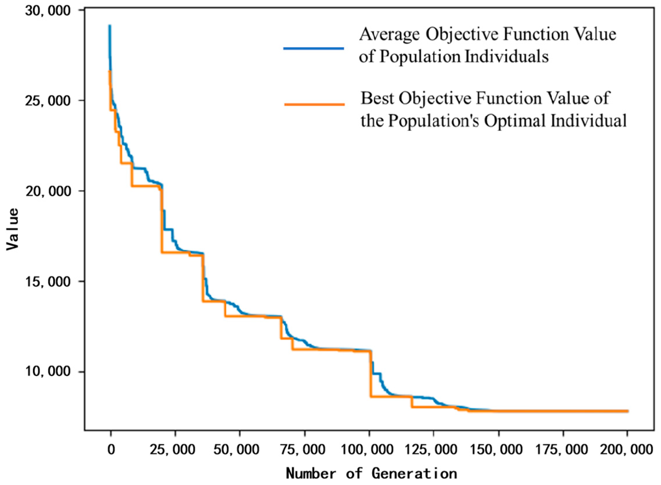
This paper establishes the optimal layout scheme of the bus network among selected stations based on the setting of weights between stations. Subsequently, synchronous optimization is conducted on the trial bus network. Following the designed algorithm, the optimization problem is solved continuously for 10 iterations, consistently yielding the optimal solution for the trial case. The convergence of the designed genetic algorithm occurs around 150,000 iterations, with subsequent results remaining unchanged. In the iteration results, although the best objective function values and average objective function values in each iteration are not exactly equal, their values are quite close. Additionally, the large y-axis values in the graph make the differences between the two close values appear insignificant, causing the best objective function values and average objective function values to look almost identical on the graph. The optimization process of the algorithm is illustrated in Figure 2.

Figure 2.
Optimization process of objective values.
4.2.2. Model Effectiveness Analysis
To further validate the effectiveness of synchronous optimization of the network and scheduling, this paper also conducts phased optimization on the selected bus network. The synchronous optimization results are compared and analyzed with the phased optimization results to study the effectiveness of the synchronous optimization model for the network and scheduling. The specific steps for phased optimization of the bus network and vehicle scheduling are as follows:
(1) Consistent with the road network basic data and passenger demand data used in synchronous optimization, optimize the bus network first with the lowest passenger time cost as the objective, considering route length, non-repeating route stations, and non-linear coefficient.
(2) Keep the optimized network unchanged, and then optimize the bus vehicle scheduling with the lowest operating cost as the objective and departure interval as the constraint, based on the optimized network.
Both phases of network optimization and scheduling setting use a genetic algorithm for model solving. In the network optimization phase, the solution obtained is the stations of the bus network, with the dimension of the solution set to match the number of network stations, which is 125. In the scheduling optimization phase, the dimension of the solution set is the number of bus routes, set to match the number of routes, which is five. Using the genetic algorithm for solving in this manner, with the model parameters and algorithm parameters consistent with synchronous optimization, the model was solved five times for each phase, resulting in optimized layouts for the bus network and corresponding departure intervals for each route after phased optimization. To ensure result accuracy, the average of the passenger time cost and operating cost from the five optimization results is taken as the phased optimization result.
By utilizing genetic algorithms to solve the synchronous optimization model, the final optimized result yields an optimal objective function value of 250,835.3 yuan. The data results for the corresponding five bus routes after synchronous optimization are shown in Table 3.
Table 3.
Synchronous optimization result data table.
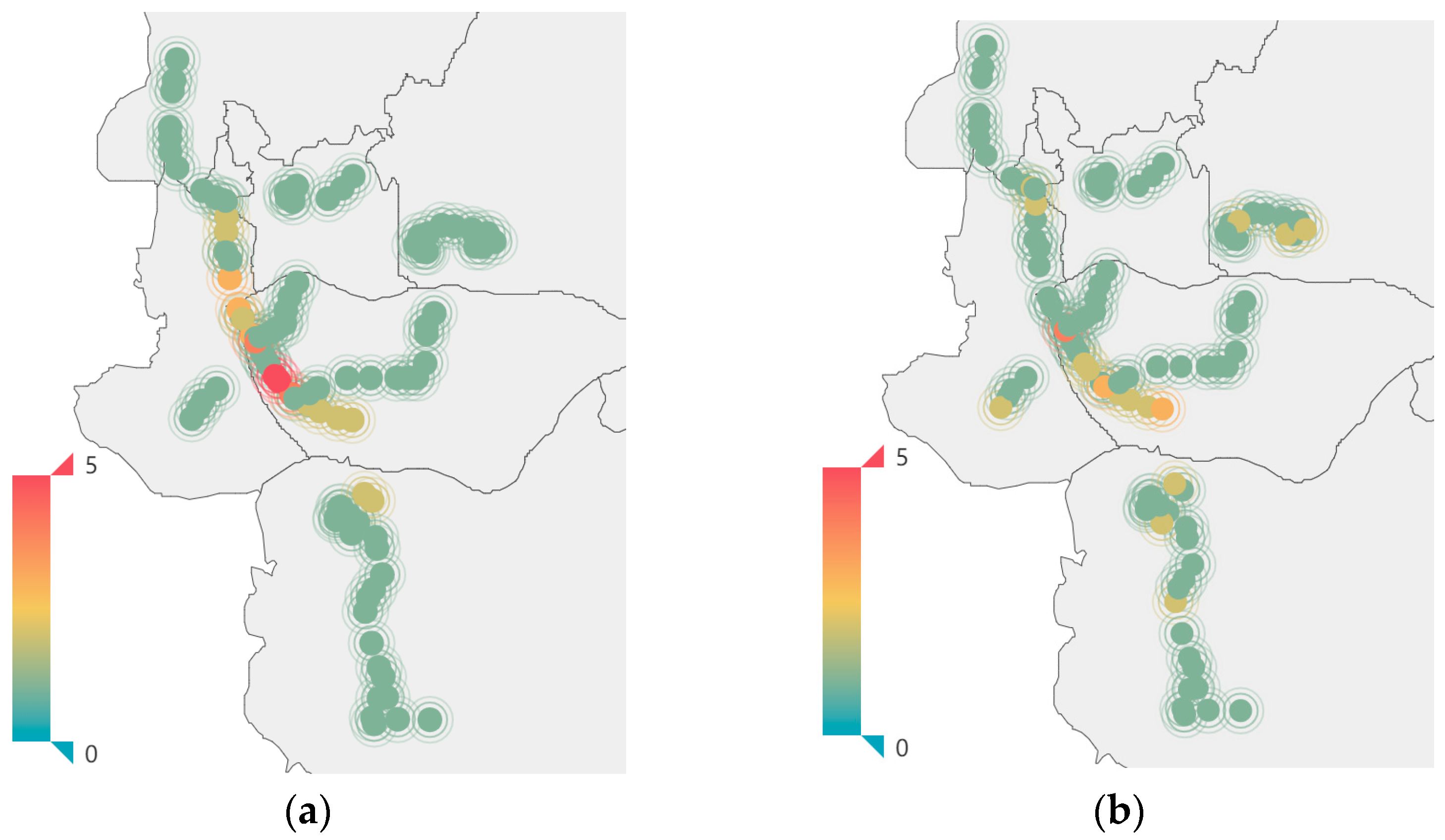
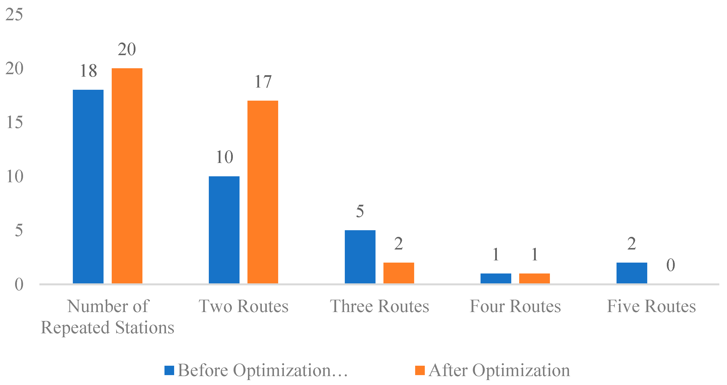
From the above chart, we can see the results of the optimization of the bus network and scheduling. The length of each route in the network is constrained to be within the range of 10 km to 30 km; the departure intervals for the vehicles on each route meet the constraint of 5 min to 15 min; the stations on each route in the network meet the non-repeating station constraint; and the non-linear coefficient for each route is below 1.4. Therefore, we conclude that the results of the optimization of the bus network and scheduling are feasible. The comparison between the heatmap of repeated station frequencies before and after optimization, as well as the comparison chart of the number of different routes and corresponding repeated station numbers before and after optimization, are shown in Figure 3 and Figure 4, respectively.
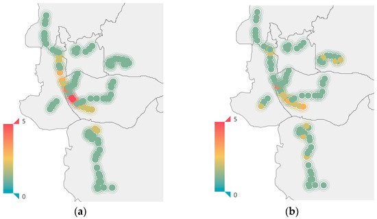
Figure 3.
(a) Optimized heatmap of repeated station frequencies before optimization. (b) Optimized heatmap of repeated station frequencies after optimization.
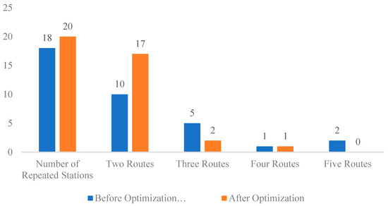
Figure 4.
Comparison chart of the number of different routes and corresponding repeated station numbers before and after optimization.
From the above figure, we can see that in the bus network stations after synchronous optimization: The number of stations existing in all five routes has decreased from two stations before optimization to zero stations. The number of stations existing in three routes has decreased from five stations before optimization to two stations. The number of stations existing in two routes has increased from 10 stations to 17 stations. The highly repeated stations in the optimized network have significantly decreased, and the repeated stations in the network are mainly concentrated on two routes, avoiding excessive route duplication and the waste of bus resources, while meeting passengers’ transfer needs during travel.
5. Discussion
This article proposes a synchronous optimization model for the bus network and scheduling, taking into account passengers’ choices of different routes during travel. Compared to previous studies, this model further refines passengers’ waiting time costs and comprehensively considers the total time cost for passengers. It also statistically analyzes passengers’ choices of different routes to better reflect real-world scenarios. Synchronous optimization is more effective than staged optimization, but there are still shortcomings that need further improvement in future research. The improvements in future research can be made in several aspects:
(1) Consideration of vehicle occupancy rates: The article assumes that passengers can all board the target route’s vehicles while waiting and does not impose capacity limits on buses. Subsequent research can introduce restrictions on the capacity of buses, such that when buses reach their full capacity, passengers need to wait for the next bus. This consideration can be incorporated into the optimization process to account for bus occupancy rates.
(2) Integration between buses and rail transit: The article only focuses on bus route deployment and does not optimize the relationship between bus routes and rail networks. With rapid development in rail transit, it has a significant impact on bus passenger flows, yet the study of the mutual influence between rail transit and buses is limited in this article. Future research can further analyze travel data between buses and rail transit, utilize bus operation data and subway ride data to study passenger flow changes, optimize the connection between buses and rail transit, and make timely adjustments to bus networks to maximize the use of public transit resources.
6. Summary
Based on the actual–virtual construction of the bus network and considering passenger waiting and on-board time, this paper further takes into account the impact of passenger route selection during travel, and establishes a synchronous optimization model for the bus network and scheduling. By conducting synchronous optimization and staged optimization on the case network separately, the results indicate that synchronous optimization is more effective than staged optimization in reducing passenger time costs and bus operation costs. Passenger time costs decreased by 21.5%, bus operation costs decreased by 13.7%, and overall bus system costs decreased by 18.0%. However, the computational complexity of the proposed model increases rapidly with the number of stations. Therefore, it is currently only suitable for optimizing bus routes in local urban areas. Future research will focus on how to apply it to truly large-scale networks.
7. Patents
The research findings of this study have been used to apply for a Chinese invention patent.
Author Contributions
Conceptualization, L.Z. (Liang Zou) and H.C.; methodology, H.C. and X.Y.; software, X.Y.; validation, X.Y.; formal analysis, L.Z. (Lingxiang Zhu); investigation, H.C.; resources, L.Z. (Liang Zou); data curation, X.Y.; writing—original draft preparation, X.Y. and L.Z. (Lingxiang Zhu); writing—review and editing, K.C. and X.Y.; visualization, L.Z. (Lingxiang Zhu) and H.C.; supervision, L.Z. (Liang Zou); funding acquisition, L.Z. (Liang Zou) All authors have read and agreed to the published version of the manuscript.
Funding
This work is supported by Shenzhen Science and Technology Plan Project (No. KJZD20230923115223047) & Shenzhen Higher Education Stable Support Plan Project (No. 20231123103157001).
Data Availability Statement
The data used to support the findings of this study are available from the corresponding author upon request.
Conflicts of Interest
Author Xi Yu was employed by the company Hangzhou Chuangtou Film and Television Co., Ltd. The remaining authors declare that the research was conducted in the absence of any commercial or financial relationships that could be construed as a potential conflict of interest.
References
- Pu, H.; Li, Y.; Ma, C. Topology analysis of Lanzhou public transport network based on double-layer complex network theory. Phys. A Stat. Mech. Its Appl. 2022, 592, 126694. [Google Scholar] [CrossRef]
- Rao, K.R.; Mitra, S.; Szmerekovsky, J. Bus Transit Network Structure Selection With Multiple Objectives. Int. J. Oper. Res. Inf. Syst. 2021, 12, 13. [Google Scholar] [CrossRef]
- Petit, A.; Yildirimoglu, M.; Geroliminis, N.; Ouyang, Y. Dedicated bus lane network design under demand diversion and dynamic traffic congestion: An aggregated network and continuous approximation model approach. Transp. Res. Part C 2021, 128, 103187. [Google Scholar] [CrossRef]
- Farahani, R.Z.; Miandoabchi, E.; Szeto, W.Y.; Rashidi, H. A review of urban transportation network design problem. Eur. J. Oper. Res. 2013, 229, 281–302. [Google Scholar] [CrossRef]
- Zhang, L.; Lu, J.; Yue, X.; Zhou, J.; Li, Y.; Wan, Q. An auxiliary optimization method for complex public transit route network based on link prediction. Mod. Phys. Lett. B 2018, 32, 1850066. [Google Scholar] [CrossRef]
- Klier, M.J.; Haase, K. Urban public transit network optimization with flexible demand. Or Spectr. 2015, 37, 195–215. [Google Scholar] [CrossRef]
- Yin, J.; D’Ariano, A.; Wang, Y.; Yang, L.; Tang, T. Timetable coordination in a rail transit network with time-dependent passenger demand. Eur. J. Oper. Res. 2021, 295, 183–202. [Google Scholar] [CrossRef]
- Liang, M.; Wang, W.; Dong, C.; Zhao, D. A cooperative coevolutionary optimization design of urban transit network and operating frequencies. Expert Syst. Appl. 2020, 160, 113736. [Google Scholar] [CrossRef]
- Wang, C.; Ye, Z.; Wang, W. A multi-objective optimization and hybrid heuristic approach for urban bus route network design. IEEE Access 2020, 8, 2154–2167. [Google Scholar] [CrossRef]
- Huang, A.; Dou, Z.; Qi, L.; Wang, L. Flexible route optimization for demand-responsive public transit service. J. Transp. Eng. Part A Syst. 2020, 146, 04020132. [Google Scholar] [CrossRef]
- Gong, M.; Hu, Y.; Chen, Z.; Li, X. Transfer-based customized modular bus system design with passenger-route assignment optimization. Transp. Res. Part E Logist. Transp. Rev. 2021, 153, 102422. [Google Scholar] [CrossRef]
- Yang, J.; Jiang, Y. Application of Modified NSGA-II to the Transit Network Design Problem. J. Adv. Transp. 2020, 2020, 3753601. [Google Scholar] [CrossRef]
- Yao, E.; Liu, T.; Lu, T.; Yang, Y. Optimization of electric vehicle scheduling with multiple vehicle types in public transport. Sustain. Cities Soc. 2020, 52, 101862. [Google Scholar] [CrossRef]
- Guo, R.; Antunes, F.; Zhang, J.; Yu, J.; Li, W. Joint optimization of headway and number of stops for bilateral bus rapid transit. PLoS ONE 2024, 19, e0300286. [Google Scholar] [CrossRef] [PubMed]
- Li, W.Y.; Gao, B.Q.; Lian, G. Microcirculation Bus Network Planning Method Based on Hierarchical Clustering. Heilongjiang Transp. Sci. Technol. 2021, 44, 166–168. [Google Scholar]
- Shi, X.W.; Su, P.T.; Zou, Y.J.; Shao, L.X. Research on Optimization of Conventional Bus Network for Rail Transit Connection Based on Shortest Path Labeling Model. Comput. Appl. Res. 2020, 37, 1–8. [Google Scholar]
- Huang, M. Multilevel Analysis of Bus Network Topological Structure. Highw. Transp. Technol. 2010, 27, 93–99. [Google Scholar]
- Yigit, F.; Basilio, M.P.; Pereira, V. A Hybrid Approach for the Multi-Criteria-Based Optimization of Sequence-Dependent Setup-Based Flow Shop Scheduling. Mathematics 2024, 12, 2007. [Google Scholar] [CrossRef]
- Ren, H.; Song, Y.; Long, J.; Si, B. A new transit assignment model based on line and node strategies. Transp. Res. Part B 2021, 150, 121–142. [Google Scholar] [CrossRef]
- Shi, Q.; Zhang, K.; Weng, J.; Dong, Y.; Ma, S.; Zhang, M. Evaluation model of bus routes optimization scheme based on multi-source bus data. Transp. Res. Interdiscip. Perspect. 2021, 10, 100342. [Google Scholar] [CrossRef]
- Fan, W.; Machemehl, R.B. Tabu search strategies for the public transportation network optimizations with variable transit demand. Comput. Aided Civ. Infrastruct. Eng. 2008, 23, 502–520. [Google Scholar] [CrossRef]
- Huang, D.; Gu, Y.; Wang, S.; Liu, Z.; Zhang, W. A two-phase optimization model for the demand-responsive customized bus network design. Transp. Res. Part C Emerg. Technol. 2020, 111, 1–21. [Google Scholar] [CrossRef]
- Li, X.; Wang, T.; Li, L.; Feng, F.; Wang, W.; Cheng, C. Joint Optimization of Regular Charging Electric Bus Transit Network Schedule and Stationary Charger Deployment considering Partial Charging Policy and Time-of-Use Electricity Prices. J. Adv. Transp. 2020, 2020, 8863905. [Google Scholar] [CrossRef]
- Steiner, K.; Irnich, S. Strategic planning for integrated mobility-on-demand and urban public bus networks. Transp. Sci. 2020, 54, 1616–1639. [Google Scholar] [CrossRef]
- Chai, S.; Liang, Q. An Improved NSGA-II Algorithm for Transit Network Design and Frequency Setting Problem. J. Adv. Transp. 2020, 2020, 2895320. [Google Scholar] [CrossRef]
- Wei, M.; Liu, T.; Sun, B.; Jing, B. Optimal integrated model for feeder transit route design and frequency-setting problem with stop selection. J. Adv. Transp. 2020, 2020, 6517248. [Google Scholar] [CrossRef]
- Tang, Z.; Hu, X.; Périaux, J. Multi-level Hybridized Optimization Methods Coupling Local Search Deterministic and Global Search Evolutionary Algorithms. Arch. Comput. Methods Eng. 2019, 27, 939–975. [Google Scholar] [CrossRef]
- Kuan, S.N.; Ong, H.L.; Ng, K.M. Solving the feeder bus network design problem by genetic algorithms and ant colony optiiTiizatiorL. Adv. Eng. Softw. 2006, 37, 351–359. [Google Scholar] [CrossRef]
- Ngamchai, S.; Lovell, D.J. Optimal time transfer in bus transit route network design using a gengtic algorithm. J. Transp. Eng. Asce 2003, 129, 510–521. [Google Scholar] [CrossRef]
- Bourbonnais, P.L.; Morency, C.; Trépanier, M.; Martel-Poliquin, É. Transit network design using a genetic algorithm with integrated road network and disaggregated O–D demand data. Transportation 2021, 48, 95–130. [Google Scholar] [CrossRef]
- Ding, J.X.; Zhong, Y.W.; Li, B.; Zhang, S. Research on Bus Network Optimization Based on Improved K-Shortest Path Algorithm. J. Hefei Univ. Technol. 2019, 42, 1388–1393+1423. [Google Scholar]
- Luo, X.L.; Jiang, S.Y. Design of Suburban Bus Network Based on K-means Clustering. Highw. Transp. Technol. 2018, 35, 115–120+134. [Google Scholar]
- Gao, M.Y.; Shi, H.G. Optimization of Rail Transit Feeder Bus Routes Based on Improved PSO Algorithm. J. Traffic Transp. Eng. Inf. 2019, 17, 49–54. [Google Scholar]
- Xin, Y.; Huo, Y.M. Multi-Objective Bus Network Optimization Model Based on NSGA-II Algorithm for Demand-Responsive Transit. Integr. Transp. 2022, 44, 68–72. [Google Scholar]
- Wang, N.; Cao, W.Z.; Chu, X.L. Optimization of Rail Transit Feeder Bus Routes using Cellular Genetic Algorithm. Transp. Technol. Econ. 2018, 20, 13–18. [Google Scholar]
- Yu, L.J.; Liang, M.P. Optimization Design of Urban Conventional Bus Network Based on Integer Nonlinear Programming. J. China Highw. 2016, 29, 108–115+135. [Google Scholar]
- Wu, K.X. Bus Network Path Optimization Based on Improved Ant Colony Algorithm. Microcomput. Appl. 2021, 37, 134–136. [Google Scholar]
- Yen, J.Y. Finding the k shortest loopless paths in a network. Manag. Sci. 1971, 17, 712–716. [Google Scholar] [CrossRef]
- Holland, J.H. Genetic algorithms. Sci. Am. 1992, 267, 44–50. [Google Scholar] [CrossRef]
Disclaimer/Publisher’s Note: The statements, opinions and data contained in all publications are solely those of the individual author(s) and contributor(s) and not of MDPI and/or the editor(s). MDPI and/or the editor(s) disclaim responsibility for any injury to people or property resulting from any ideas, methods, instructions or products referred to in the content. |
© 2024 by the authors. Licensee MDPI, Basel, Switzerland. This article is an open access article distributed under the terms and conditions of the Creative Commons Attribution (CC BY) license (https://creativecommons.org/licenses/by/4.0/).