Multilevel Hierarchical Bayesian Modeling of Cross-National Factors in Vehicle Sales

Abstract

SUVs (sport utility vehicles), as a car segment, have become a foundation within the automotive industry due to their versatility, which is used by a wide range of customers. Recognising the complex interplay between geographical and economic conditions across countries, we delve into cross-national factors that significantly influence SUV sales. This article presents an analysis of the global sales of SUVs (sport utility vehicles) using multilevel hierarchical Bayesian modelling. We identify key predictors of SUV sales, including the effects of fuel prices, income levels and geographical aspects. We prepared four statistical models that differ in their probability distribution or hierarchical internal structure. The last presented model, with Student’s t-distribution and separate distribution for unique alpha parameter values, turned out to be the best one. Our analysis contributes to a deeper understanding of the automotive market dynamics, and it can also assist manufacturers and policymakers in designing effective sales strategies.

1. Introduction

SUVs (sport utility vehicles), as a car segment, have become a foundation within the automotive industry due to their versatility. Initially designed for challenging terrains and poor road conditions, today’s SUVs cater to a broad spectrum of needs, offering models that range from compact urban crossovers to full-sized luxury cars. Their adaptability makes them perfect for families requiring extra space, outdoor enthusiasts in need of toughness, and those looking for a symbol of status and sophistication. The SUV market continues to grow, with manufacturers extending their current range of new models or engine versions to better suit customer needs.

Following North America in the last decade, the trend can likewise be seen in Europe. A great example of this is Poland, where, despite the end of the pandemic, galloping inflation and the ever-increasing cost of living, SUV sales continue to grow by the year. In 2022, they accounted for as much as 46.4% of all new car registrations [1]. Based on Figure 1, which uses the previous year’s data, seven of the top ten best-selling passenger cars were SUVs. Furthermore, this type of car is usually considerably more expensive to buy than the other classic body types, which further prompts a consideration of what factors might have influenced purchasers’ decisions for these types of cars. Their rising popularity and utility drove our focus on SUVs.

The problem we focused on investigating was the impact of economic and geographical factors on SUV sales, and we generated a model that predicts these sales. We chose to study whether aspects such as the quality of infrastructure, geographical location and a country’s welfare do, in fact, determine whether this type of car is sold more or less often.

There are many ways to predict car sales, but very few of them focus on SUVs. Indian scientists, in an article, discussed the development of a machine learning model to predict whether a customer would buy an SUV based on data collected from banks [3]. The model applies logistic regression to analyse data on customer age and estimated salary to forecast their purchasing behaviour. In addition, they explored various machine learning and data mining techniques used to handle the chosen issue. It was the only article we found that focused on the creation of an SUV sales prediction model. Another interesting and popular approach to general car purchase prediction is the reliance on sentiment analysis. The main difference between them is the sources of analysed data. Some individuals base their analysis on information collected from car review websites and social media [4], whereas others additionally incorporate data derived from Google Trends [5].

In view of the possible approaches, we chose to use Bayesian inference. It is a statistical technique that combines prior knowledge with new data to make forecasts about uncertain events, based on Bayes’s rule. We rely on it to update the likelihood of an event in the case of getting more information about it [6]. This approach not only offers an estimate but also quantifies the uncertainty around it, providing a full probability distribution for the parameters being studied. The key advantage of this approach lies in its adaptability, which comes from its ability to incorporate various levels of randomness and merge information from different sources while considering all plausible sources of uncertainty in inferential summaries. Bayesian methods tend to create smoothed estimates in complex data structures, which improves their capacity to deliver more accurate responses that reflect real-world situations. Moreover, Bayesian inferences depend on probability models that inevitably include simplifications when attempting to depict complex real-world interactions and relationships. If Bayesian responses significantly vary based on scientifically sound assumptions that cannot be disputed based on the data, then the range of potential conclusions should be recognised as valid [7].

The main goal was to create and train relevant Bayesian models with the use of MCMC (Markov-chain Monte Carlo) sampling. We can distinguish between several types of Bayesian models, classified according to the number of parameters, their structure or the distributions used. The variety of models prepared for our project provided us with an equally diverse approach and a broader view of the issue. In light of this, we created four different models based on various distributions and structures. Furthermore, models characterised by multiple levels are called hierarchical [7].

The paper is structured as follows: The second part (materials and methods) introduces two prepared datasets and the structure of the models with their prior predictive check. The third part (results) illustrates and analyses the data obtained from models. The fourth part (discussion and conclusions) compares the models using two different criteria and then draws conclusions and outlines future development opportunities.

2. Materials and Methods

2.1. Datasets

We start with a description of the prepared dataset obtained from [8] (

Table 1. Example records from SUV sales dataset [8].

Country	SUV Sales	Road Quality	Mountain Area	Wage	Fuel Price
Argentina	16.13	3.60	30.00	427.94	0.90
Australia	50.65	4.90	6.00	4218.89	1.35
Brazil	21.82	3.00	30.00	402.77	1.29
Canada	43.00	5.00	24.00	3338.62	1.18
China	30.98	4.60	33.00	1122.36	1.19

).

We focused on infrastructure, geographical location and a country’s welfare as our main areas of interest. SUVs are often more expensive to buy and maintain than classic sedans or hatchback cars. Moreover, this type of car has significantly higher fuel consumption. As a result of their size and weight, they need more powerful engines with a larger cylinder capacity. Therefore, we chose the average salary and the average fuel price in a country as factors that could influence purchasing decisions. Another key fact is SUVs’ off-road capability, which also determines their convenience. People’s places of residence, or more precisely, their geographical locations, sometimes force them to have cars with raised ground clearance and four-wheel drive for their everyday lives. This suggested to us that we should include the road quality indicator and a country’s mountain coverage as sales determinants. In addition to information on the percentage of SUVs among the newly sold cars in a country, our dataset contains the following:

• The average income per person (in USD), based on CEOWORLD magazine’s research about average monthly net salaries around the world from 2022;
• The quality of road infrastructure (on a scale from 1 to 7), based on information from the World Economic Forum 2019;
• Average fuel prices (in USD), based on information from the portal Numbeo.com from 2023;
• The percentage of a country’s area covered in mountains, based on information from the non-profit environmental foundation GRID-Arendal.

2.1.1. Dataset 1—49 Countries

Dataset 1 contains data from 49 different countries, the majority of which are European. The data came mainly from articles by JATO Dynamics, a global automotive market research company, or from statista.com, a statistics portal for market data. More detailed information on the several sources used for the data can be found in the dataset’s GitHub repository [8]. It is visualised in Figure 2.

2.1.2. Dataset 2—G20

The diversity of the countries in Dataset 1, both economically and geographically, affected the performance of statistical models. Thus, we decided to prepare a second dataset with the G20 (Group of 20) countries. The G20 is a series of intergovernmental forums to discuss common financial policies. This group consists of 19 countries and the EU (European Union) [9]. These are the countries considered to be the most important economically worldwide, which will make it possible, at least in economic terms, to minimise the impact of diversity on the results obtained. The data for individual countries were taken from Dataset 1, while the information for the EU was calculated as the average of all EU countries in Dataset 1.

2.2. Modelling

Bayesian statistics is a powerful inference framework that uses Bayes’s theorem to update the probability of a hypothesis as new data become available, and it incorporates uncertainty in the inference process. Its flexibility allows for representing data with multiple classes of models (represented by likelihoods); each of those considers different types of parameters, which have their own models (represented with prior distributions). Therefore, we prepared four different models. They enabled us to comprehensively compare of 3 diverse probability distributions using various hierarchies of parameters.

For each of the created models, both datasets were used in order to additionally validate their efficiency on a smaller set of closer values. All models had the same input data, which were the number of data points appropriate for the dataset (forty-nine for the main set and twenty for the G20 one), SUV sales and further factorial details from the dataset. For Bayesian modelling, it is good practice to execute prior and posterior predictive checks for the sampled model. Both are efficient verification techniques. The first of them allowed for the confirmation of which data we should anticipate based on our current knowledge without putting observed data into our model. In other words, the results from a prior predictive check rely only on the given parameters. On the contrary, posterior predictive checks determine whether, after the model is updated with real data, it returns the correct output data in relation to the observed ones [10]. It is part of the final model validation.

2.2.1. Model 1

The first model was chosen as a Gaussian Linear Model (denoted as the first model):

$$\begin{array}{cc}\hfill \alpha & \sim \mathrm{Normal}(0,0.25)\hfill \\ \hfill {\beta }_{fp}& \sim \mathrm{Normal}(0,0.25)\hfill \\ \hfill {\beta }_w& \sim \mathrm{Normal}(0,0.25)\hfill \\ \hfill {\beta }_{rq}& \sim \mathrm{Normal}(0,0.25)\hfill \\ \hfill {\beta }_{ma}& \sim \mathrm{Normal}(0,0.25)\hfill \\ \hfill \sigma & \sim \mathrm{HalfNormal}(0,0.1)\hfill \end{array}$$

(1)

$$\begin{array}{cc}\hfill {\mu }_i& =\alpha +{\beta }_{fp}·f{p}_i+{\beta }_w·w_i+{\beta }_{rq}·r{q}_i+{\beta }_{ma}·m{a}_i\hfill \end{array}$$

(2)

$$\begin{array}{cc}\hfill y_i& \sim \mathrm{Normal}({\mu }_i,\sigma )\hfill \\ \hfill \end{array}$$

(3)

where the following applies:

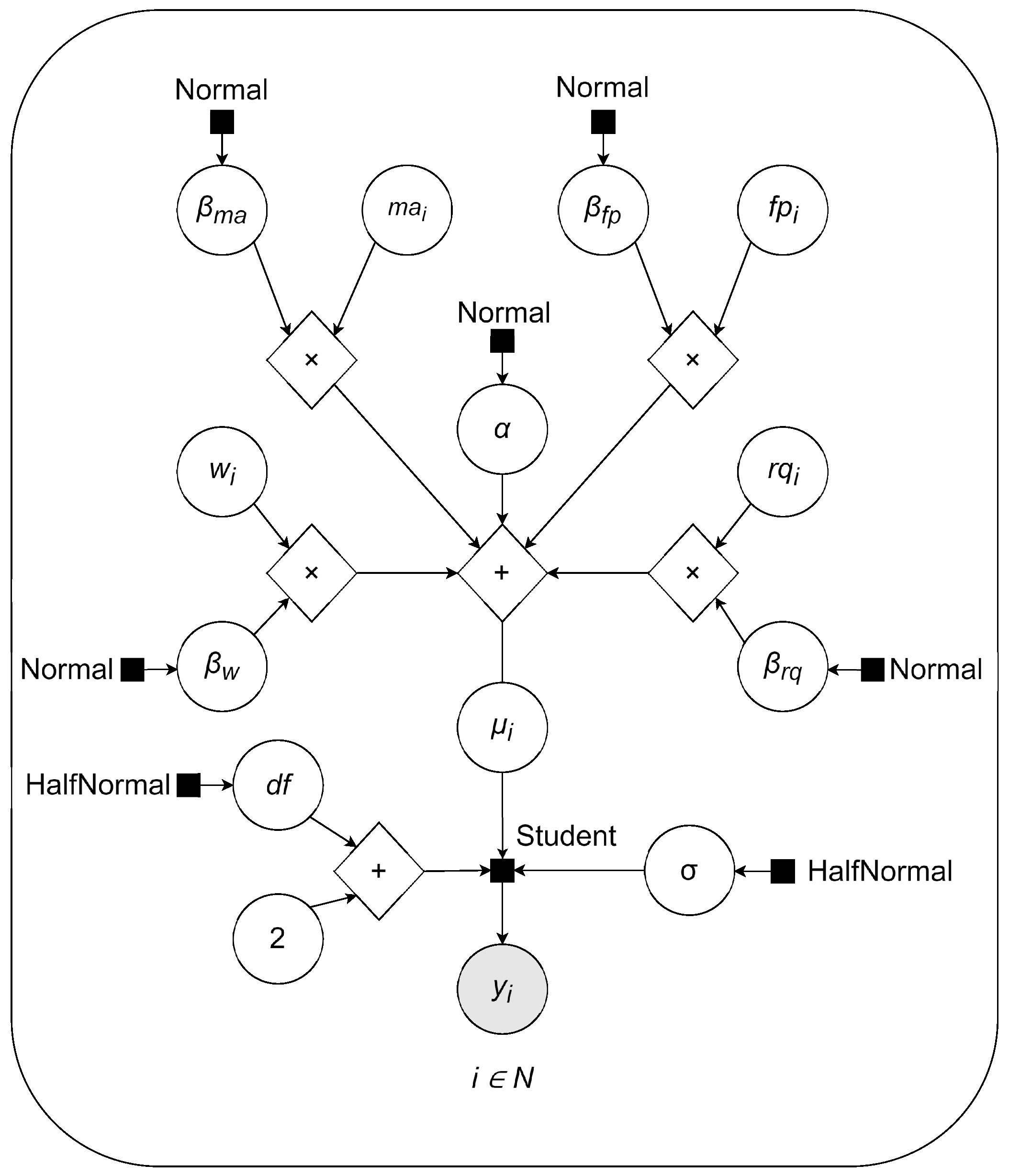
• $\alpha$ is the intercept of the model.
• ${\beta }_{fp}$ is the coefficient for the effect of fuel prices on the response variable.
• ${\beta }_w$ is the coefficient for the effect of wages on the response variable.
• ${\beta }_{rq}$ is the coefficient for the effect of road quality on the response variable.
• ${\beta }_{ma}$ is the coefficient for the effect of mountainous terrain on the response variable.
• $\sigma$ is the square root of the standard deviation of the main distribution in the model.
• ${\mu }_i$ is the mean response for the i-th observation.
• ${fp}_i$, $w_i$, ${rq}_i$, and ${ma}_i$ are the observed values of fuel prices, wages, road quality, and mountainous areas, respectively, for the i-th observation.
• $y_i$ is the response variable of SUV sales for the i-th observation.

The model was based on the normal distribution with the parameter $\mu$, responsible for the expected value of SUV sales [11]. The block model calculates the transformed parameters as a linear combination of the predictors weighted according to their respective coefficients, (2). In comparison to $\sigma$, defined as a scalar, $\mu$ is calculated separately for each data point and stored in a vector, as is the subsequently predicted sales value. Furthermore, this equation was the starting point for each of the subsequent models.

Figure 3 emphasises the simplicity of the model structure. The whole model relies on a direct calculation of the parameters of a single normal distribution. Moreover, all minor coefficients are also determined using Gaussian distribution. For coefficients and intercept distributions, we assumed standardised parameters: a mean of zero and a deviation of fractional values of one divided by the number of factors included in the model. In our case, this fraction was a quarter. The distribution for the sigma parameter stood out from that of the others. The reason for this is the fact that a standard deviation should have a smaller value in relation to the mean value in the normal distribution.

Firstly, we executed the prior predictive check. The procedure was the same for all models. We sampled the model (or, more precisely, its version prepared for the prior predictive check) 2000 times. In the next step, we created an individual histogram of the output distribution for each country and placed the actual value on this graph. In that way, we verified whether the real data were achievable and whether it was possible to determine with the chosen specification and model parameters. Furthermore, in this visualisation, we could observe whether the model returned any anomalous outliers from the assumptions made. If the analysed model had a more complicated, hierarchical structure, histograms of the indirect parameters were also added. We can observe in Figure 4 that the shape of the histogram of our first model’s output, as expected, shows a normal distribution. Its mean is around zero, and the values for the three example countries are achievable, which allowed us to proceed with a further examination of the model.

2.2.2. Model 2

One of the main objectives of the project was a sales prediction for SUVs, a specific type of car, as a percentage of all new cars registered in a given country. In this case, our distribution was supposed to be based on values analogous to percentages—values from 0 to 1. That is what the beta distribution provided us with [12]. Similarly to the first model, our starting point was the linear combination of predictors (2), but this time, it was not a direct parameter of the final distribution:

$$\begin{array}{cc}\hfill \alpha & \sim \mathrm{Normal}(0,1)\hfill \\ \hfill {\beta }_{fp}& \sim \mathrm{Normal}(0,0.25)\hfill \\ \hfill {\beta }_w& \sim \mathrm{Normal}(0,0.25)\hfill \\ \hfill {\beta }_{rq}& \sim \mathrm{Normal}(0,0.25)\hfill \\ \hfill {\beta }_{ma}& \sim \mathrm{Normal}(0,0.25)\hfill \end{array}$$

(4)

$$\begin{array}{cc}\hfill \eta & \sim \mathrm{Uniform}(0,50)\hfill \\ \hfill {\mu }_i& =\alpha +{\beta }_{fp}·f{p}_i+{\beta }_w·w_i+{\beta }_{rq}·r{q}_i+{\beta }_{ma}·m{a}_i\hfill \end{array}$$

(5)

$$\begin{array}{cc}\hfill {{\alpha }_{param}}_i& ={\mu }_i·\eta \hfill \end{array}$$

(6)

$$\begin{array}{cc}\hfill {{\beta }_{param}}_i& =(1-{\mu }_i)·\eta \hfill \end{array}$$

(7)

$$\begin{array}{cc}\hfill {var}_i& ={\displaystyle \frac{{\mu }_i·(1-{\mu }_i)}{\eta +1}}\hfill \end{array}$$

(8)

$$\begin{array}{cc}\hfill y_i& \sim \mathrm{Beta}({{\alpha }_{param}}_i,{{\beta }_{param}}_i)\hfill \\ \hfill \end{array}$$

(9)

where the following applies:

• $\eta$ is the dispersion parameter of the beta distribution.
• ${{\alpha }_{param}}_i$ is the first direct parameter for the beta distribution.
• ${{\beta }_{param}}_i$ is the second direct parameter for the beta distribution.
• $va{r}_i$ is the value of variance for the beta distribution.

Model is visualised if the Figure 5.

Instead of the previously known standard deviation, we introduced the dispersion parameter $\eta$ [13]. In our model case, its value was initialised using a uniform distribution (5). Subsequently, we calculated the direct distribution parameters ${\alpha }_{param}$ and ${\beta }_{param}$ based on the determined mean and dispersion values (6) and (7) [14]. In addition to the equations essential to our beta regression, for verification purposes, we also computed the values of variance for every model sample (8) [15]. Regarding coefficients of the beta factor, the distributions were unchanged from the first model.

Let us move on to the prior predictive check from Figure 6. It was executed in the same way as the first model. However, a significant difference can be noted in the obtained results. The influence of the beta distribution caused the output values to be between only zero and one. The values were distributed quite centrally with an increase in the number of values from the middle of the interval, which was reminiscent of the previously used normal distribution, but this time, it was limited at the ends. The real sales values, which are percentages, were obviously within the range of the output. It is remarkable to note the significantly higher value bar located next to the actual value in each of the graphs.

As mentioned in the previous paragraph, the major element of the model’s verification was also to check the distributions of its internal parameters. For the second model, we prepared a subplot containing ${\alpha }_{param}$, ${\beta }_{param}$ and variance histograms for each of the considered countries. Figure 7 shows an example histogram for Albania. All values of ${\alpha }_{param}$ and ${\beta }_{param}$ were noticeably limited to zero and, therefore, non-negative. This is one of the requirements which the beta distribution imposed on us. On the other hand, the variance achieved low values, which is proof of not much difference in the output values. It may indicate that the model can be adapted less effectively to outliers.

2.2.3. Model 3

Student’s t-distribution resembled classic Gaussian distribution. The main difference between them is their “tails”: Student’s tails are much heavier. This attribute allows for more relevance in cases with unknown variance or smaller populations [16]. Our problem of sales prediction fit these criteria. For the next model, we went back to the initial assumptions in (1), although we used another new probability distribution, Student’s t-distribution:

$$\begin{array}{cc}\hfill \alpha & \sim \mathrm{Normal}(0,1)\hfill \\ \hfill {\beta }_{fp}& \sim \mathrm{Normal}(0,0.25)\hfill \\ \hfill {\beta }_w& \sim \mathrm{Normal}(0,0.25)\hfill \\ \hfill {\beta }_{rq}& \sim \mathrm{Normal}(0,0.25)\hfill \end{array}$$

(10)

$$\begin{array}{cc}\hfill {\beta }_{ma}& \sim \mathrm{Normal}(0,0.25)\hfill \\ \hfill \sigma & \sim \mathrm{HalfNormal}(0,0.1)\hfill \\ \hfill df& \sim \mathrm{HalfNormal}(0,20)\hfill \\ \hfill {\mu }_i& =\alpha +{\beta }_{fp}·f{p}_i+{\beta }_w·w_i+{\beta }_{rq}·r{q}_i+{\beta }_{ma}·m{a}_i\hfill \end{array}$$

(11)

$$\begin{array}{cc}\hfill y_i& \sim \mathrm{Student}(df+2,{\mu }_i,\sigma ))\hfill \\ \hfill \end{array}$$

(12)

where the following applies:

• $df$ is the degrees of freedom parameter of Student’s t-distribution.

In contrast to Gaussian distribution, for Student’s t-distribution, we need three input parameters, which forced us to add another variable to the model, (10), and obviously to modify the main distribution for the output data, (12). Beyond the mean and variance, it was additionally parameterised according to the degrees of freedom. Their number was responsible for the width of the distribution. The lower the number of degrees, the wider Student’s t-distribution and the higher its tails. Like other variables, it was initialised with a normal distribution.

The structure of the model is fairly straightforward, and Figure 8 strongly resembles Figure 3.

Similar to the structure and diagram, the output from the prior predictive check was similar in appearance to that of the first model. The histograms were Gaussian-shaped and symmetric around zero. The vast majority of values were close to zero, although the equivalent first model’s graphs from Figure 9 had a much tighter range of possible values. Contrary to the second model, there were negative output values. For each of the three example countries, the observed data were among the most commonly received values, which led us to high expectations for the model’s predictive effectiveness.

2.2.4. Model 4

The fourth model is an extension of the third model, based on the same distribution. In our primary assumptions, for each model so far, the intercept $\alpha$ was a scalar. In other words, it assumed the same value for each of the predicted countries. As we can observe based on the SUV sales percentage differences between countries in the original dataset, presented in the Figure 2, it is not the best solution. That is why we decided to change our strategy for the last model.

In order to diversify the alpha values, we introduced the following model:

$$\begin{array}{cc}\hfill {{\gamma }_{param}}_i& \sim \mathrm{Normal}(0,1)\hfill \end{array}$$

(13)

$$\begin{array}{cc}\hfill {{\delta }_{param}}_i& \sim \mathrm{HalfNormal}(0,0.1)\hfill \\ \hfill {\alpha }_i& \sim \mathrm{Normal}({{\gamma }_{param}}_i,{{\delta }_{param}}_i)\hfill \\ \hfill {\beta }_{fp}& \sim \mathrm{Normal}(0,0.25)\hfill \\ \hfill {\beta }_w& \sim \mathrm{Normal}(0,0.25)\hfill \\ \hfill {\beta }_{rq}& \sim \mathrm{Normal}(0,0.25)\hfill \end{array}$$

(14)

$$\begin{array}{cc}\hfill {\beta }_{ma}& \sim \mathrm{Normal}(0,0.25)\hfill \\ \hfill \sigma & \sim \mathrm{HalfNormal}(0,0.1)\hfill \\ \hfill df& \sim \mathrm{HalfNormal}(0,20)\hfill \\ \hfill {\mu }_i& ={\alpha }_i+{\beta }_{fp}·f{p}_i+{\beta }_w·w_i+{\beta }_{rq}·r{q}_i+{\beta }_{ma}·m{a}_i\hfill \\ \hfill y_i& \sim \mathrm{Student}(df+2,{\mu }_i,\sigma )\hfill \\ \hfill \end{array}$$

(15)

where the following applies:

• ${{\gamma }_{param}}_i$ is a mean value parameter for the intercept $\alpha$’s normal distribution.
• ${{\delta }_{param}}_i$ is a variance parameter for the intercept $\alpha$’s normal distribution.

We replaced alpha distribution parameters with another output of another two distributions (15). For ${{\gamma }_{param}}_i$ and ${{\delta }_{param}}_i$, we opted for normal distributions with the following regular parameters: a mean value equal to zero for both and a smaller variance value for the one responsible for the variance itself. The other factor distributions remained unchanged from the previous model, which was well represented through the similarity of the diagrams from Figure 8 and Figure 10.

The implementation of a parameterised intercept resulted in changes in the appearance of the model’s prior predictive check (see Figure 11). The histograms do not resemble the characteristic symmetric, normal-distribution bell shape. The range of values shifted towards positive values, and the vast majority were positive, too. Furthermore, the distribution’s peak was between zero and one, and the same applied to the sales percentage data. Similar to the second model, the observed values of the displayed countries were close to their histogram’s summit.

3. Results

The section concerning the results’ presentation merits starting with the technical aspects of the implementation. The entire project was written in Python 3.11 with CmdStanPy 1.2.4, an interface for Stan. Stan is a programming language dedicated to solving probabilistic problems using statistical inference [17]. Instead of a local environment, we used Google Colaboratory—a cloud-based platform with a Jupyter Notebook environment, which allows users to write and execute their Python code. All code prepared as part of this project, like the datasets, was shared and is available in a separate repository [18]. Each model has its own notebook containing data pre-processing, detailed prior predictive checks, model sampling and posterior predictive checks.

3.1. Comparison of Models

After model sampling, we moved on to the posterior model outputs. For every model, we attached an error-bar graph with a comparison of the predicted and actual sales values for two sampled datasets—the G20 dataset and an extended one with forty-nine countries. As a predicted value, we took the mean of the country’s output distribution. Additionally, for the larger set, we prepared the world map plot in the same form as original set visualised in the Figure 2. This visualisation allowed for a better observation and illustration of the differences between expected and received values.

3.1.1. Results for Model 1

Figure 12 shows error-bar plots obtained for Model 1. The blue bars indicate real sales; meanwhile, the black points with error bars represent the predicted sales values with their standard deviations. Starting from the top, we noticed that, in many cases, the output model aligned closely with the real values. On the other hand, there were notable deviations, like for Thailand or Argentina, where the predicted sales were significantly underestimated compared to the real ones. It looks very similar in the second posted graph. Out of twenty countries, we had at least three that were undervalued: Russia, Saudi Arabia and South Africa.

Comparing the maps from Figure 2 and Figure 13, we concluded that the second map displays lower sales for several countries, particularly in Europe and parts of Asia. It is also hard to talk about the diversity of values. The vast majority of countries have a similar shade and, consequently, comparable sales values. Overall, the model’s predictions can be rated as moderately accurate, with a reasonable output across various countries. However, significant deviations in a few cases indicate the need for model refinements and suggest room for an improvement in prediction accuracy.

3.1.2. Results for Model 2

Figure 14 shows the comparison of the second model outputs for two datasets. The results are very close to those obtained from the previous model. The values are comparable to each other; most of them are achievable, but there are some underestimated cases. Nevertheless, comparing the results between two considered datasets, we find that, for both of them, the model returned approximate values with equally similar predictive efficiency.

The world map for the second model (Figure 15) is nearly identical to the first model’s map. Most of the continents are covered with the same shade of blue colour, representing SUVs as fifty per cent of car sales. For effective world map visualisation, we definitely need more value diversity. Otherwise, this type of chart cannot offer a valuable comparison. The inclusion of the second model in the plots compared with the previous one reveals that further model improvements are still required.

3.1.3. Results for Model 3

The choice of a new distribution did not significantly improve the accuracy compared to Model 3’s (see Figure 16). Once again, for many countries from the larger dataset, the forecasts were close to the actual results. It is worth mentioning that the differences between the means of the model outputs for each country were scant. All of them fell in the range of 0.3 to 0.4. We are able to see standard deviations in the width spectrum, showing us the undervaluation of the output model. The error bar for Norway’s sales prediction stands out, particularly with its wide scope.

The world map for the third model is the first one of those we discussed in which there are observable colour differences. We can notice them, for example, by comparing the area of Australia for this Figure 17 and the previous Figure 15. Unfortunately, these are not clear differences that would allow us to intuitively use the map as a comparative visualisation.

3.1.4. Results for Model 4

As we can see in Figure 18, the values obtained from Model 4 are precise and relevant, and the standard deviation ranges are strongly reduced by the range, indicating a high quality of prediction. The model provides a reasonable estimation of SUV sales percentages.

The bar chart set high expectations for how the map would look for the fourth model, and these were definitely fulfilled (see Figure 19). It is certainly the closest approximation to the map with real data from Figure 2. We can distinguish differences in values based on the various shades. Outliers such as very low sales in Brazil and Argentina or far-above-average sales, such as in Norway or Spain, are also accurately highlighted. In this respect, Model 4 provides better results than any of the other models.

4. Discussion and Conclusions

4.1. Discussion

The WAIC (Watanabe–Akaike Information Criterion) is a model criterion based on the log-likelihood function. Its estimation process consists of employing the ELPD (Expected Log Predictive Density) for a new data point calculation and then applying a correction for over-fitting [7]. A ranking plot shows the ELPD values for each model. The model with the best predictive precision is believed to have the highest ELPD value.

In Figure 20, we noticed that, during graph generation, the models were sorted. The better-ranked ones (with a higher ELPD) were higher. The WAIC plot only confirms the effectiveness of the fourth model. It has the highest ELPD, indicating that it has the best predictive accuracy. The remaining models took comparable values. Besides the points themselves, the plot also contains error bars and ELPD difference symbols.

The second criterion under our consideration was LOO-CV (Leave-One-Out Cross-Validation). It is based on the mean of predicted errors across all points in the dataset. For a single data point, this error was calculated as follows (iteratively for each dataset point) [7]:

• The point is skipped;
• The model is fitted again, without the omitted point, to the rest of the data;
• The predicted error is calculated for the missing point.

According to Figure 21, due to the highest ELPD, the fourth model has the best predictive accuracy again. The second and third models have fairly close ELPD values. The remaining model with number one has significantly low efficiency. The error bars indicate the range within which the ELPD difference is likely to fall, reflecting the uncertainty in this comparison. The consistency in ranking between both criteria can further affirm a model’s performance.

The results obtained for the fourth model prove the effectiveness of using a unique alpha distribution for each of the samples. It allows for more flexibility by introducing more parameters and, therefore, more probability distributions. Originally, we also wanted to conduct a similar procedure only for the beta distribution based on the second model, but due to the problematic learning of the model, we abandoned this approach.

Comparing our results with other existing models in the literature is challenging due to the absence of models that cover the same factors analysed in this article. This unique approach distinguishes our work and highlights the novelty of our research. Our study was intended to fill this gap and pave the way for future development.

4.2. Conclusions and Future Work

In this paper, we built four multilevel Bayesian hierarchical models. Each of these allowed us to obtain acceptable results based solely on the values of various factors and suitable probability distributions. The last one of the models deserves supplementary recognition. Using Student’s t-distribution provided outputs that were only negligibly different from the real data.

Moreover, every model used a fusion of data on various aspects of SUVs’ popularity, including geographical and economic data. A thorough analysis of this phenomenon and research enabled us to select the most important factors affecting the sales of those cars. In addition to the ones highlighted and included in the models’ parameters, there is also a large number of non-measurable cultural and social factors, such as attachment, feelings or social status.

An inherent facet in the model’s possible development is the extension of the additional parameters. It is highly probable that new factors and data will appear, having a significant impact on the calculated predictive values. Furthermore, the performance of the models for a different dataset will be worth checking. In the case of our project, we chose to analyse a global dataset mainly because of data availability. These types of models are usually applied to more narrow and similar sets. However, in our posterior predictive sample, the predictions for a smaller G20 set returned significantly more precise values. As mentioned, our models were used in a more global context, although sales analyses are likely to be conducted from a local perspective. Therefore, it will be worthwhile to examine our models’ accuracy for the regional issue if a relevant dataset is collected. For example, SUV sales for only European countries or states in the United States would provide a noteworthy analysis. It would allow a focus on a smaller dataset and, in particular, more comparable values for the measurable factors and a similar cultural background. Undoubtedly, this would have a positive influence on the potential results.

To address the deviations between model predictions and actual sales, as well as the potential reduction in explanatory power with increased complexity, we propose several future development strategies. These include involving industry experts to refine model assumptions, expanding the dataset to include more countries and time periods for better generalizability, and incorporating socio-cultural factors. Additionally, exploring advanced statistical and machine learning techniques, as well as implementing rigorous cross-validation methods, would potentially help optimize the model’s performance in predicting SUV sales.

Our study predominantly examined economic and geographical factors affecting SUV sales. However, socio-cultural elements, such as consumer preferences and social status symbols, also play significant roles. These factors can deeply influence purchasing decisions and market trends. Future research should integrate these dimensions to enhance the model’s predictive capabilities. Collaborating with sociologists or other specialists and utilising more comprehensive data could provide valuable insights into the cultural and social dynamics driving SUV sales across various parts of the world.

Knowing this type of information can give essential insights into car distribution patterns and trends in population behaviours regarding car investment in specific areas of the globe. Those insights can be used to predict future car sales or even impact the number of produced vehicles itself. Moreover, it can help car manufacturers develop all kinds of sales, marketing or promotional strategies through ways to target customers from certain regions of the world.

References

1. Poland Car Sales Data—Sales of New Cars in Poland, 2024. Based on the Data from Manufactures, ANDC (Automotive News Data Center) and JATO Dynamics. Available online: https://www.goodcarbadcar.net/poland-car-sales-data/ (accessed on 16 April 2024).
2. Registrations of New Cars and Light Commercial Vehicles up to 3.5 T: January–December 2023. Press Release. 2024. Available online: https://www.pzpm.org.pl/pl/content/download/14071/93625/file/PZPM_CEP_Info_SOiSD_09_2023.pdf (accessed on 16 April 2024).
3. Geetharamani, G.; Dhinakaran, K.; Selvaraj, J.; Singh, S. Sport-utility vehicle prediction based on machine learning approach. J. Appl. Res. Technol. 2021, 19, 184–193. [Google Scholar] [CrossRef]
4. Punjabi, S.K.; Shetty, V.; Pranav, S.; Yadav, A. Sales Prediction using Online Sentiment with Regression Model. In Proceedings of the 2020 4th International Conference on Intelligent Computing and Control Systems (ICICCS), Madurai, India, 13–15 May 2020; pp. 209–212. [Google Scholar]
5. Wijnhoven, F.; Plant, O. Sentiment Analysis and Google Trends Data for Predicting Car Sales; University of Twente: Enschede, The Netherlands, 2017. [Google Scholar]
6. Berger, J.O. Statistical Decision Theory and Bayesian Analysis, 2nd ed.; Springer series in statistics; Springer: Berlin/Heidelberg, Germany, 2011. [Google Scholar]
7. Gelman, A.; Carlin, J.B.; Stern, H.S.; Rubin, D.B. Bayesian Data Analysis; Chapman and Hall/CRC: Boca Raton, FL, USA, 1995. [Google Scholar]
8. SUV Sales Determination Dataset GitHub Repository. 2024. Available online: https://github.com/sukiennik-monika/SUV-Sales-Determination-Dataset (accessed on 16 April 2024).
9. Hajnal, P.I. The G20: Evolution, Interrelationships, Documentation; Taylor & Francis: Abingdon, UK, 2019. [Google Scholar]
10. Lee, M.D.; Wagenmakers, E.J. Bayesian Cognitive Modeling: A Practical Course; Cambridge University Press: Cambridge, UK, 2014. [Google Scholar]
11. Lambert, B. A Student’s Guide to Bayesian Statistics; Sage Publications Ltd.: Thousand Oaks, CA, USA, 2018; pp. 1–520. [Google Scholar]
12. Ferrari, S.; Cribari-Neto, F. Beta regression for modelling rates and proportions. J. Appl. Stat. 2004, 31, 799–815. [Google Scholar] [CrossRef]
13. Bayesian Beta Regression. 2023. Available online: https://m-clark.github.io/models-by-example/bayesian-beta-regression.html (accessed on 16 April 2024).
14. Kruschke, J. Doing Bayesian Data Analysis: A Tutorial with R, JAGS, and Stan; Academic Press: Cambridge, MA, USA, 2014. [Google Scholar]
15. Cribari-Neto, F.; Zeileis, A. Beta regression in R. J. Stat. Softw. 2010, 34, 1–24. [Google Scholar] [CrossRef]
16. Hurst, S. The Characteristic Function of the Student t-Distribution; Centre for Mathematics and Its Applications, School of Mathematical Sciences, ANU: Canberra, Australia, 1995. [Google Scholar]
17. Stan Docs—Stan User’s Guide. 2024. Available online: https://mc-stan.org/docs/stan-users-guide/ (accessed on 16 April 2024).
18. Bayesian Models for SUV Sales Determination GitHub Repository. 2024. Available online: https://github.com/sukiennik-monika/Bayesian-Modeling-Of-Cross-National-Factors-In-SUV-Sales (accessed on 9 May 2024).
Figure 1. Top 10 best-selling passenger cars in Poland in 2023 [2].
Applsci 14 06325 g001
Figure 2. World map with real data about SUVs as a percentage of the newly sold cars in countries.
Applsci 14 06325 g002
Figure 3. Diagram of the structure of the linear regression model (first model).
Applsci 14 06325 g003
Figure 4. Prior predictive check for three example countries from the linear regression model (first model). The red line indicates the true SUV sales percentage value for the displayed country. In prior predictive checks (PPCs), we allowed for negative values and a spread of values; the main point of prior selection was ensuring that real data were possible under prior assumptions and providing a sampler with the necessary flexibility in the parameter space.
Applsci 14 06325 g004
Figure 5. Diagram of the structure of the model with beta distribution (second model).
Applsci 14 06325 g005
Figure 6. Prior predictive check for three example countries from the model with beta distribution (second model). The red line indicates the true SUV sales percentage value for the displayed country. In prior predictive checks (PPCs), we allowed for negative values and a spread of values; the main point of the prior selection was ensuring that real data were possible under prior assumptions and providing the sampler with the necessary flexibility in the parameter space.
Applsci 14 06325 g006
Figure 7. Histograms of indirect parameters for a single example country from the model with beta distribution (second model).
Applsci 14 06325 g007
Figure 8. Diagram of the structure of the model with Student’s t-distribution (third model).
Applsci 14 06325 g008
Figure 9. Prior predictive check for three example countries from the model with Student’s t-distribution (third model). The red line indicates the true SUV sales percentage value for the displayed country. In prior predictive checks (PPCs), we allowed for negative values and a spread of values; the main point of the prior selection was ensuring that real data were possible under prior assumptions and providing a sampler with the necessary flexibility in the parameter space.
Applsci 14 06325 g009
Figure 10. Diagram of the structure of the model with Student’s t-distribution and unique alpha values (fourth model).
Applsci 14 06325 g010
Figure 11. Prior predictive check for the model with Student’s t-distribution and unique alpha values (fourth model). The red line indicates the true SUV sales percentage value for the displayed country. In prior predictive checks (PPCs), we allowed for negative values and a spread of values; the main point of the prior selection was ensuring that real data were possible under prior assumptions and providing a sampler with the necessary flexibility in the parameter space.
Applsci 14 06325 g011
Figure 12. Comparison plot with the predicted and actual SUV sales values for the linear regression model (first model).
Applsci 14 06325 g012
Figure 13. World map with the output data from the linear regression model (first model).
Applsci 14 06325 g013
Figure 14. Comparison plot with the predicted and actual SUV sales values for a model with beta distribution (the second model).
Applsci 14 06325 g014
Figure 15. World map with the output data from the model with beta distribution (second model).
Applsci 14 06325 g015
Figure 16. Comparison plot with the predicted and actual SUV sales values for the model with Student’s t-distribution (third model).
Applsci 14 06325 g016
Figure 17. World map with the output data from the model with Student’s t-distribution (third model).
Applsci 14 06325 g017
Figure 18. Comparison plot with the predicted and actual SUV sales values for the model with Student’s t-distribution and unique alpha values (fourth model).
Applsci 14 06325 g018
Figure 19. World map with the output data from the model with Student’s t-distribution and unique alpha values (fourth model).
Applsci 14 06325 g019
Figure 20. Model comparison using WAIC.
Applsci 14 06325 g020
Figure 21. Model comparison using LOO-CV.
Applsci 14 06325 g021