
Joint Luminance Adjustment and Color Correction for Low-Light Image Enhancement Network

Abstract
1. Introduction
2. Related Work
2.1. Luminance Adjustment in Low-Light Image Enhancement
2.2. Color Correction in Low-Light Image Enhancement
3. Method
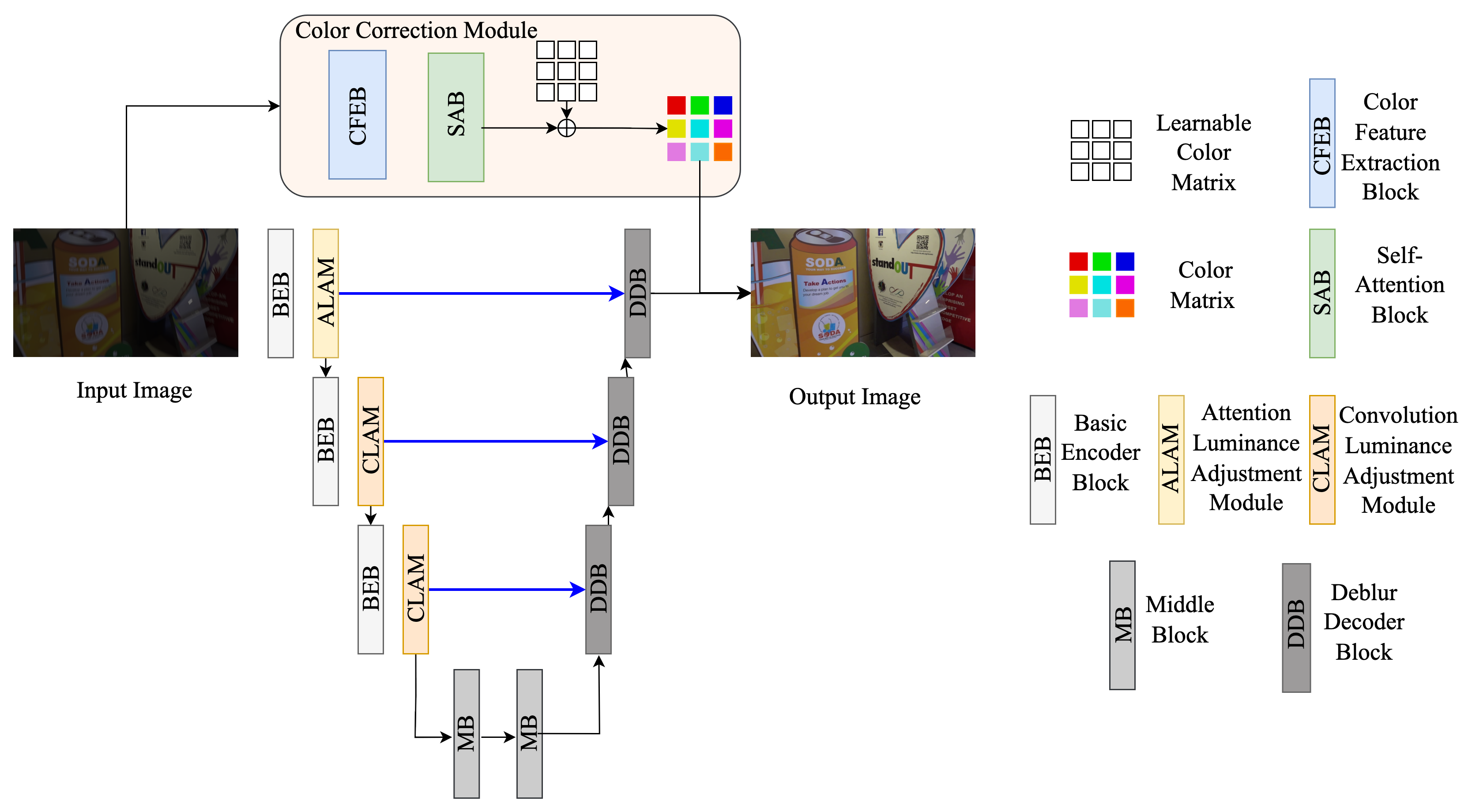
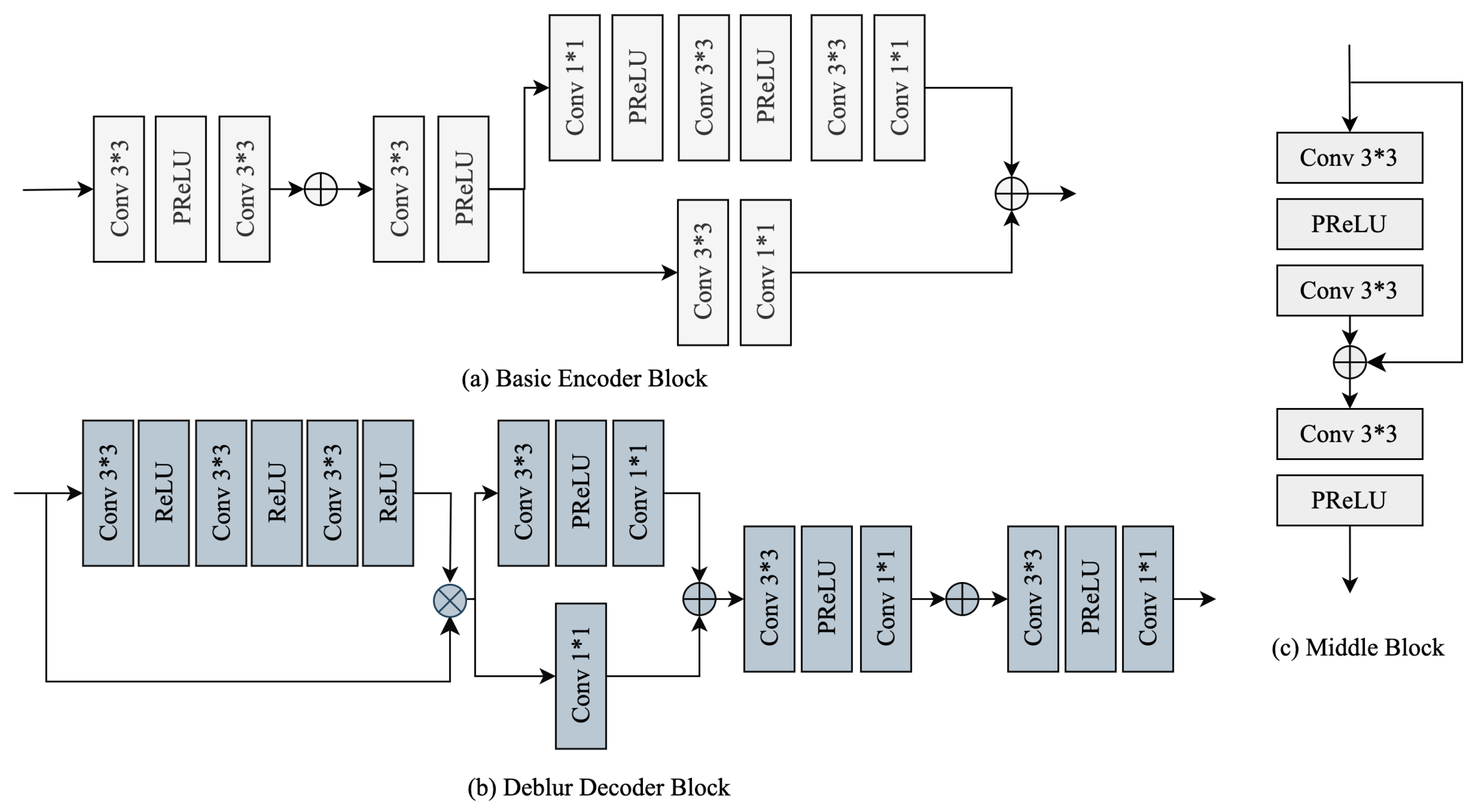
3.1. Framework
3.2. Luminance Adjustment Module
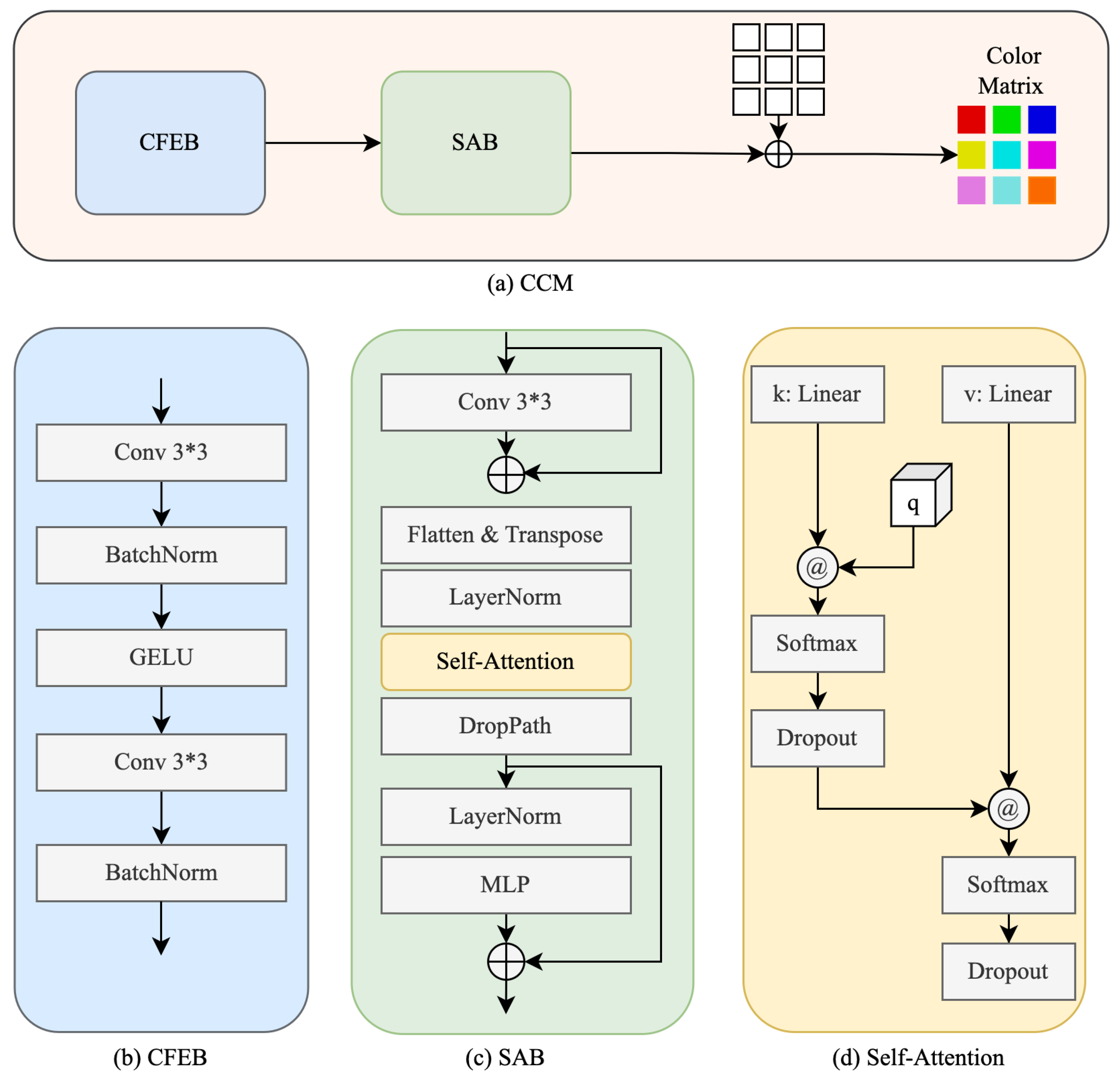
3.3. Color Correction Module
3.4. Loss Functions
4. Experiments
4.1. Datasets
4.2. Experiment Settings
4.3. Quantitative Evaluation
4.3.1. Peak Signal-to-Noise Ratio (PSNR)
4.3.2. Structural Similarity Index (SSIM)
4.3.3. Learned Perceptual Image Patch Similarity (LPIPS)
4.3.4. Natural Image Quality Evaluator (NIQE)
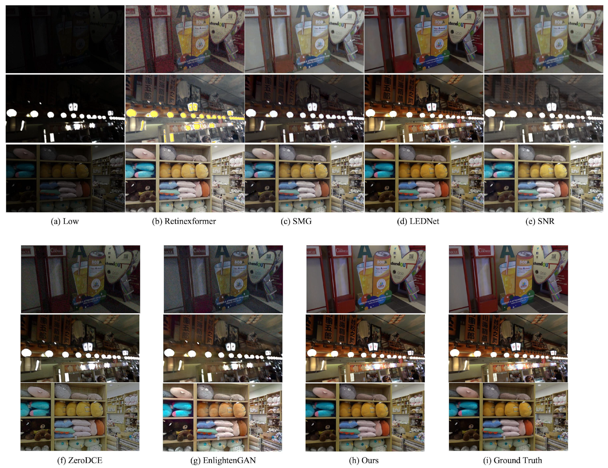
4.4. Comparison with State-of-the-Art Methods
4.5. Ablation Experiments
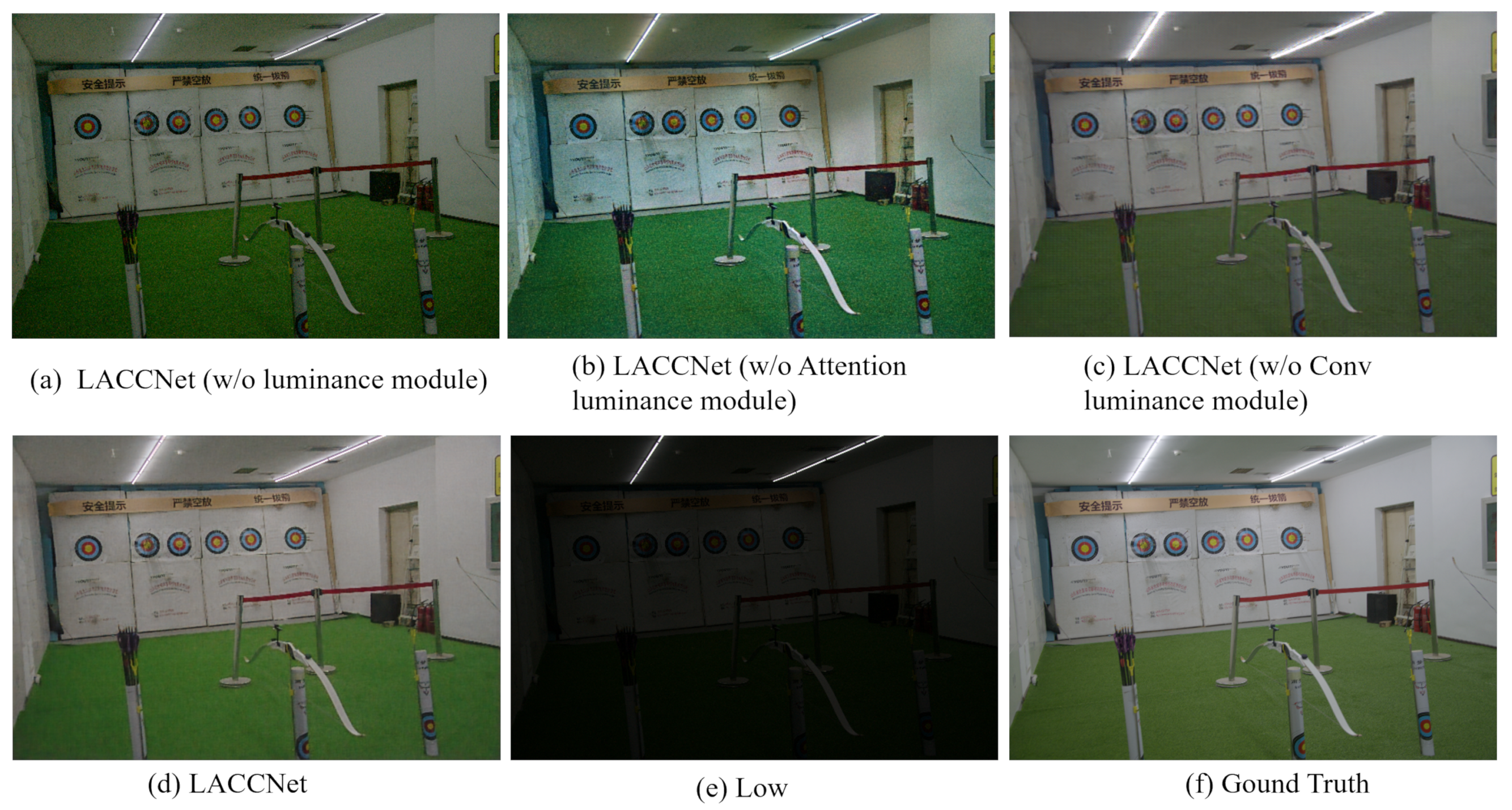
4.5.1. Effectiveness Analysis of Luminance Adjustment Module
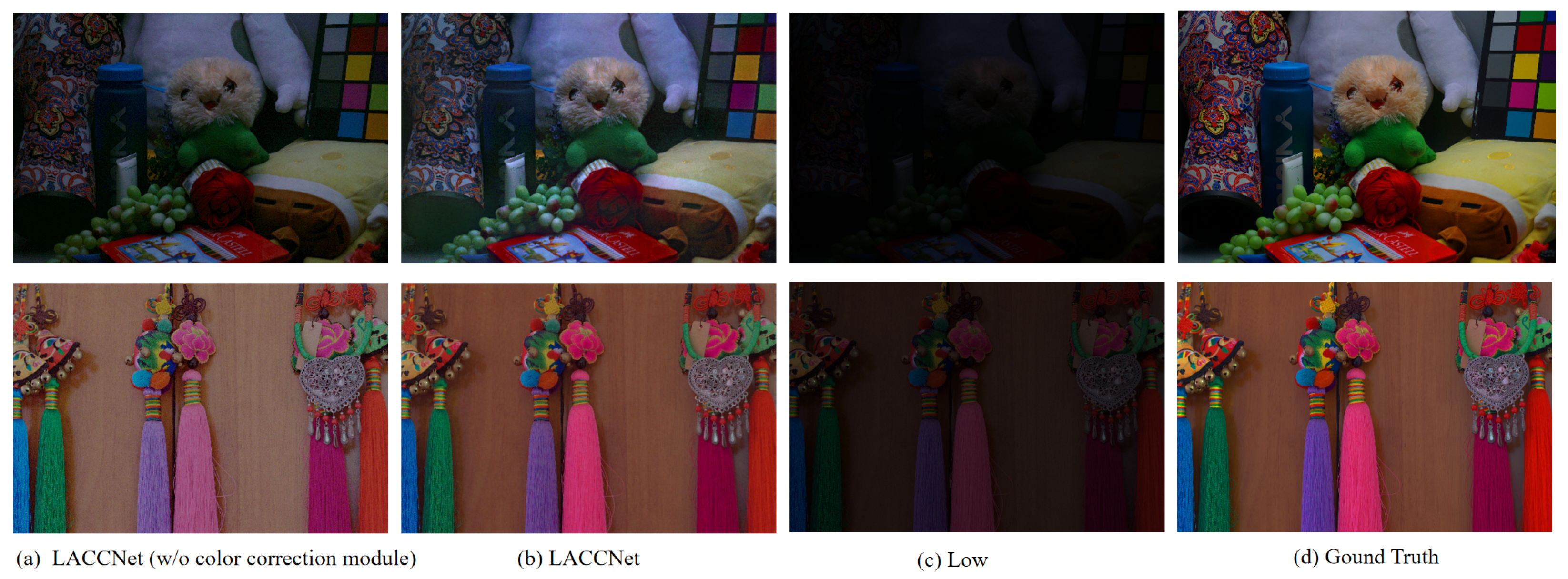
4.5.2. Effectiveness Analysis of Color Correction Module
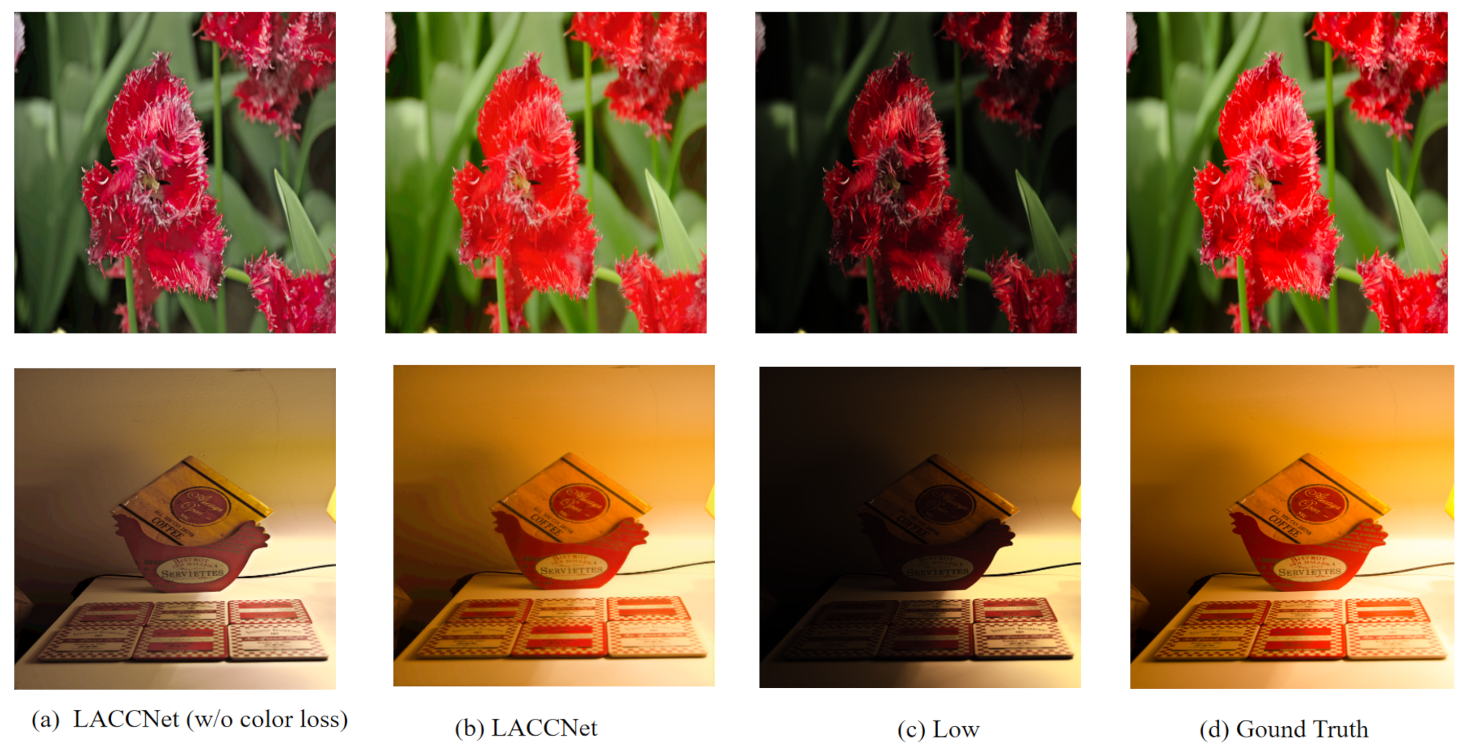
4.5.3. Effectiveness Analysis of Color Loss Function
5. Conclusions
Author Contributions
Funding
Institutional Review Board Statement
Informed Consent Statement
Data Availability Statement
Conflicts of Interest
References
- Wang, J.; Li, Y.; Cao, L.; Li, Y.; Li, N.; Gao, H. Range-restricted pixel difference global histogram equalization for infrared image contrast enhancement. Opt. Rev. 2021, 28, 145–158. [Google Scholar] [CrossRef]
- Abdullah-Al-Wadud, M.; Kabir, M.H.; Dewan, M.A.A.; Chae, O. A dynamic histogram equalization for image contrast enhancement. IEEE Trans. Consum. Electron. 2007, 53, 593–600. [Google Scholar] [CrossRef]
- Dong, X.; Pang, Y.; Wen, J. Fast efficient algorithm for enhancement of low lighting video. In Proceedings of the 2011 IEEE International Conference on Multimedia and Expo, Barcelona, Spain, 11–15 July 2011; pp. 1–6. [Google Scholar]
- Li, D.; Shi, H.; Wang, H.; Liu, W.; Wang, L. Image Enhancement Method Based on Dark Channel Prior. In Proceedings of the 2022 International Conference on Computer Engineering and Artificial Intelligence (ICCEAI), Shijiazhuang, China, 22–24 July 2022; pp. 200–204. [Google Scholar]
- Jobson, D.J.; Rahman, Z.u.; Woodell, G.A. Properties and performance of a center/surround retinex. IEEE Trans. Image Process. 1997, 6, 451–462. [Google Scholar] [CrossRef] [PubMed]
- Rahman, Z.u.; Jobson, D.J.; Woodell, G.A. Multi-scale retinex for color image enhancement. In Proceedings of the 3rd IEEE International Conference on Image Processing, Lausanne, Switzerland, 19 September 1996; Volume 3, pp. 1003–1006. [Google Scholar]
- Guo, X.; Li, Y.; Ling, H. LIME: Low-light image enhancement via illumination map estimation. IEEE Trans. Image Process. 2016, 26, 982–993. [Google Scholar] [CrossRef] [PubMed]
- Ren, X.; Yang, W.; Cheng, W.H.; Liu, J. LR3M: Robust low-light enhancement via low-rank regularized retinex model. IEEE Trans. Image Process. 2020, 29, 5862–5876. [Google Scholar] [CrossRef] [PubMed]
- Wei, C.; Wang, W.; Yang, W.; Liu, J. Deep retinex decomposition for low-light enhancement. arXiv 2018, arXiv:1808.04560. [Google Scholar]
- Wang, T.; Zhang, K.; Shao, Z.; Luo, W.; Stenger, B.; Kim, T.K.; Liu, W.; Li, H. LLDiffusion: Learning degradation representations in diffusion models for low-light image enhancement. arXiv 2023, arXiv:2307.14659. [Google Scholar]
- Zhou, D.; Yang, Z.; Yang, Y. Pyramid diffusion models for low-light image enhancement. arXiv 2023, arXiv:2305.10028. [Google Scholar]
- Ni, Z.; Yang, W.; Wang, H.; Wang, S.; Ma, L.; Kwong, S. Cycle-interactive generative adversarial network for robust unsupervised low-light enhancement. In Proceedings of the 30th ACM International Conference on Multimedia, Lisboa, Portugal, 10 October 2022; pp. 1484–1492. [Google Scholar]
- Guo, C.; Li, C.; Guo, J.; Loy, C.C.; Hou, J.; Kwong, S.; Cong, R. Zero-reference deep curve estimation for low-light image enhancement. In Proceedings of the IEEE/CVF Conference on Computer Vision and Pattern Recognition, Seattle, WA, USA, 13 June 2020; pp. 1780–1789. [Google Scholar]
- Li, C.; Guo, C.; Loy, C.C. Learning to enhance low-light image via zero-reference deep curve estimation. IEEE Trans. Pattern Anal. Mach. Intell. 2021, 44, 4225–4238. [Google Scholar] [CrossRef] [PubMed]
- Wu, W.; Weng, J.; Zhang, P.; Wang, X.; Yang, W.; Jiang, J. Uretinex-net: Retinex-based deep unfolding network for low-light image enhancement. In Proceedings of the IEEE/CVF Conference on Computer Vision and Pattern Recognition, New Orleans, LA, USA, 18 June 2022; pp. 5901–5910. [Google Scholar]
- Wang, Y.; Yu, Y.; Yang, W.; Guo, L.; Chau, L.P.; Kot, A.C.; Wen, B. Exposurediffusion: Learning to expose for low-light image enhancement. In Proceedings of the IEEE/CVF International Conference on Computer Vision, Paris, France, 2–6 October 2023; pp. 12438–12448. [Google Scholar]
- Wen, J.; Wu, C.; Zhang, T.; Yu, Y.; Swierczynski, P. Self-Reference Deep Adaptive Curve Estimation for Low-Light Image Enhancement. arXiv 2023, arXiv:2308.08197. [Google Scholar]
- Zhang, Y.; Zhang, J.; Guo, X. Kindling the darkness: A practical low-light image enhancer. In Proceedings of the 27th ACM International Conference on Multimedia, Nice, France, 21–25 October 2019; pp. 1632–1640. [Google Scholar]
- Zhang, Y.; Guo, X.; Ma, J.; Liu, W.; Zhang, J. Beyond brightening low-light images. Int. J. Comput. Vis. 2021, 129, 1013–1037. [Google Scholar] [CrossRef]
- Jobson, D.J.; Rahman, Z.u.; Woodell, G.A. A multiscale retinex for bridging the gap between color images and the human observation of scenes. IEEE Trans. Image Process. 1997, 6, 965–976. [Google Scholar] [CrossRef] [PubMed]
- Wang, H.; Xu, X.; Xu, K.; Lau, R.W. Lighting up nerf via unsupervised decomposition and enhancement. In Proceedings of the IEEE/CVF International Conference on Computer Vision, Paris, France, 2–6 October 2023; pp. 12632–12641. [Google Scholar]
- Yang, S.; Ding, M.; Wu, Y.; Li, Z.; Zhang, J. Implicit neural representation for cooperative low-light image enhancement. In Proceedings of the IEEE/CVF International Conference on Computer Vision, Paris, France, 2–6 October 2023; pp. 12918–12927. [Google Scholar]
- Jia, X.; De Brabandere, B.; Tuytelaars, T.; Gool, L.V. Dynamic filter networks. Adv. Neural Inf. Process. Syst. 2016, 29, 667–675. [Google Scholar]
- Liu, Z.; Lin, Y.; Cao, Y.; Hu, H.; Wei, Y.; Zhang, Z.; Lin, S.; Guo, B. Swin transformer: Hierarchical vision transformer using shifted windows. In Proceedings of the IEEE/CVF International Conference on Computer Vision, Montreal, QC, Canada, 10–17 October 2021; pp. 10012–10022. [Google Scholar]
- Zhou, S.; Li, C.; Change Loy, C. Lednet: Joint low-light enhancement and deblurring in the dark. In Proceedings of the European Conference on Computer Vision, Tel-Aviv, Israel, 23–27 October 2022; pp. 573–589. [Google Scholar]
- Yang, W.; Wang, W.; Huang, H.; Wang, S.; Liu, J. Sparse gradient regularized deep retinex network for robust low-light image enhancement. IEEE Trans. Image Process. 2021, 30, 2072–2086. [Google Scholar] [CrossRef] [PubMed]
- Hai, J.; Xuan, Z.; Yang, R.; Hao, Y.; Zou, F.; Lin, F.; Han, S. R2rnet: Low-light image enhancement via real-low to real-normal network. J. Vis. Commun. Image Represent. 2023, 90, 103712. [Google Scholar] [CrossRef]
- Cai, J.; Gu, S.; Zhang, L. Learning a deep single image contrast enhancer from multi-exposure images. IEEE Trans. Image Process. 2018, 27, 2049–2062. [Google Scholar] [CrossRef] [PubMed]
- Lee, C.; Lee, C.; Kim, C.S. Contrast enhancement based on layered difference representation of 2D histograms. IEEE Trans. Image Process. 2013, 22, 5372–5384. [Google Scholar] [CrossRef] [PubMed]
- Ma, K.; Zeng, K.; Wang, Z. Perceptual quality assessment for multi-exposure image fusion. IEEE Trans. Image Process. 2015, 24, 3345–3356. [Google Scholar] [CrossRef] [PubMed]
- Mittal, A.; Soundararajan, R.; Bovik, A.C. Making a ’Completely Blind’ Image Quality Analyzer. IEEE Signal Process. Lett. 2013, 20, 209–212. [Google Scholar] [CrossRef]
- Cai, Y.; Bian, H.; Lin, J.; Wang, H.; Timofte, R.; Zhang, Y. Retinexformer: One-stage retinex-based transformer for low-light image enhancement. In Proceedings of the IEEE/CVF International Conference on Computer Vision, Paris, France, 2–3 October 2023; pp. 12504–12513. [Google Scholar]
- Xu, X.; Wang, R.; Lu, J. Low-light image enhancement via structure modeling and guidance. In Proceedings of the IEEE/CVF Conference on Computer Vision and Pattern Recognition, Vancouver, Canada, 18–22 June 2023; pp. 9893–9903. [Google Scholar]
- Xu, X.; Wang, R.; Fu, C.W.; Jia, J. Snr-aware low-light image enhancement. In Proceedings of the IEEE/CVF Conference on Computer Vision and Pattern Recognition, New Orleans, LA, USA, 18–24 June 2022; pp. 17714–17724. [Google Scholar]
- Jiang, Y.; Gong, X.; Liu, D.; Cheng, Y.; Fang, C.; Shen, X.; Yang, J.; Zhou, P.; Wang, Z. Enlightengan: Deep light enhancement without paired supervision. IEEE Trans. Image Process. 2021, 30, 2340–2349. [Google Scholar] [CrossRef] [PubMed]


| Methods | LOL-Blur | LOL-V1 | ||||
|---|---|---|---|---|---|---|
| PSNR | SSIM | LPIPS | PSNR | SSIM | LPIPS | |
| Retinexformer | 17.525 | 0.686 | 0.455 | 25.160 | 0.845 | 0.252 |
| SMG | 19.669 | 0.746 | 0.429 | 24.306 | 0.893 | 0.308 |
| LEDNet | 25.740 | 0.850 | 0.224 | 14.857 | 0.746 | 0.374 |
| SNR | 16.191 | 0.687 | 0.431 | 24.610 | 0.842 | 0.257 |
| Zero-DCE | 18.448 | 0.643 | 0.481 | 14.861 | 0.681 | 0.372 |
| EnlightenGAN | 16.677 | 0.633 | 0.478 | 17.555 | 0.733 | 0.381 |
| LACCNet (Ours) | 26.728 | 0.841 | 0.199 | 24.388 | 0.870 | 0.227 |
| Methods | LOL-V2-real | LOL-V2-syn | LSRW | ||||||
|---|---|---|---|---|---|---|---|---|---|
| PSNR | SSIM | LPIPS | PSNR | SSIM | LPIPS | PSNR | SSIM | LPIPS | |
| Retinexformer | 22.800 | 0.840 | 0.288 | 25.670 | 0.930 | 0.105 | 17.779 | 0.537 | 0.407 |
| SMG | 24.620 | 0.867 | 0.293 | 25.620 | 0.905 | 0.156 | 18.081 | 0.636 | 0.384 |
| LEDNet | 18.752 | 0.783 | 0.392 | 18.612 | 0.811 | 0.258 | 16.508 | 0.521 | 0.424 |
| SNR | 21.480 | 0.849 | 0.261 | 24.140 | 0.928 | 0.087 | 17.653 | 0.579 | 0.496 |
| Zero-DCE | 18.058 | 0.705 | 0.352 | 17.756 | 0.845 | 0.178 | 15.857 | 0.472 | 0.417 |
| EnlightenGAN | 18.684 | 0.740 | 0.368 | 16.486 | 0.811 | 0.226 | 17.592 | 0.508 | 0.404 |
| LACCNet (Ours) | 24.711 | 0.869 | 0.259 | 24.921 | 0.869 | 0.198 | 20.087 | 0.672 | 0.359 |
| Methods | LOL-Blur | LOL-V1 | LOL-V2-real | LOL-V2-syn | LSRW | DICM |
|---|---|---|---|---|---|---|
| Retinexformer | 4.715 | 3.489 | 3.966 | 4.022 | 3.481 | 3.686 |
| SMG | 7.285 | 6.131 | 5.858 | 6.123 | 6.156 | 6.139 |
| LEDNet | 4.764 | 5.491 | 5.358 | 5.093 | 4.832 | 4.789 |
| SNR | 8.241 | 5.217 | 4.638 | 4.129 | 7.215 | 4.643 |
| Zero-DCE | 5.088 | 7.496 | 7.666 | 4.392 | 3.698 | 3.954 |
| EnlightenGAN | 4.779 | 4.778 | 5.156 | 4.073 | 3.320 | 3.570 |
| Ours | 4.685 | 4.897 | 3.912 | 3.986 | 3.294 | 3.589 |
| Modules | Networks | PSNR | SSIM | LPIPS | NIQE |
|---|---|---|---|---|---|
| LAM | LACCNet (w/o LAM) | 23.50 | 0.71 | 0.41 | 5.71 |
| LACCNet (w/o ALAM) | 25.96 | 0.81 | 0.36 | 5.09 | |
| LACCNet (w/o CLAM) | 24.75 | 0.79 | 0.39 | 5.38 | |
| CCM | LACCNet (w/o CCM) | 23.19 | 0.75 | 0.29 | 4.77 |
| Color Loss | LACCNet (w/o Color Loss) | 23.32 | 0.69 | 0.35 | 4.92 |
| LACCNet | 26.73 | 0.84 | 0.20 | 4.69 |
Disclaimer/Publisher’s Note: The statements, opinions and data contained in all publications are solely those of the individual author(s) and contributor(s) and not of MDPI and/or the editor(s). MDPI and/or the editor(s) disclaim responsibility for any injury to people or property resulting from any ideas, methods, instructions or products referred to in the content. |
© 2024 by the authors. Licensee MDPI, Basel, Switzerland. This article is an open access article distributed under the terms and conditions of the Creative Commons Attribution (CC BY) license (https://creativecommons.org/licenses/by/4.0/).
Share and Cite
Zhang, N.; Han, X.; Liu, C.; Gang, R.; Ma, S.; Cao, Y. Joint Luminance Adjustment and Color Correction for Low-Light Image Enhancement Network. Appl. Sci. 2024, 14, 6320. https://doi.org/10.3390/app14146320
Zhang N, Han X, Liu C, Gang R, Ma S, Cao Y. Joint Luminance Adjustment and Color Correction for Low-Light Image Enhancement Network. Applied Sciences. 2024; 14(14):6320. https://doi.org/10.3390/app14146320
Chicago/Turabian StyleZhang, Nenghuan, Xiao Han, Chenming Liu, Ruipeng Gang, Sai Ma, and Yizhen Cao. 2024. "Joint Luminance Adjustment and Color Correction for Low-Light Image Enhancement Network" Applied Sciences 14, no. 14: 6320. https://doi.org/10.3390/app14146320
APA StyleZhang, N., Han, X., Liu, C., Gang, R., Ma, S., & Cao, Y. (2024). Joint Luminance Adjustment and Color Correction for Low-Light Image Enhancement Network. Applied Sciences, 14(14), 6320. https://doi.org/10.3390/app14146320