


Site-Specific Deterministic Temperature and Dew Point Forecasts with Explainable and Reliable Machine Learning


Abstract
1. Introduction
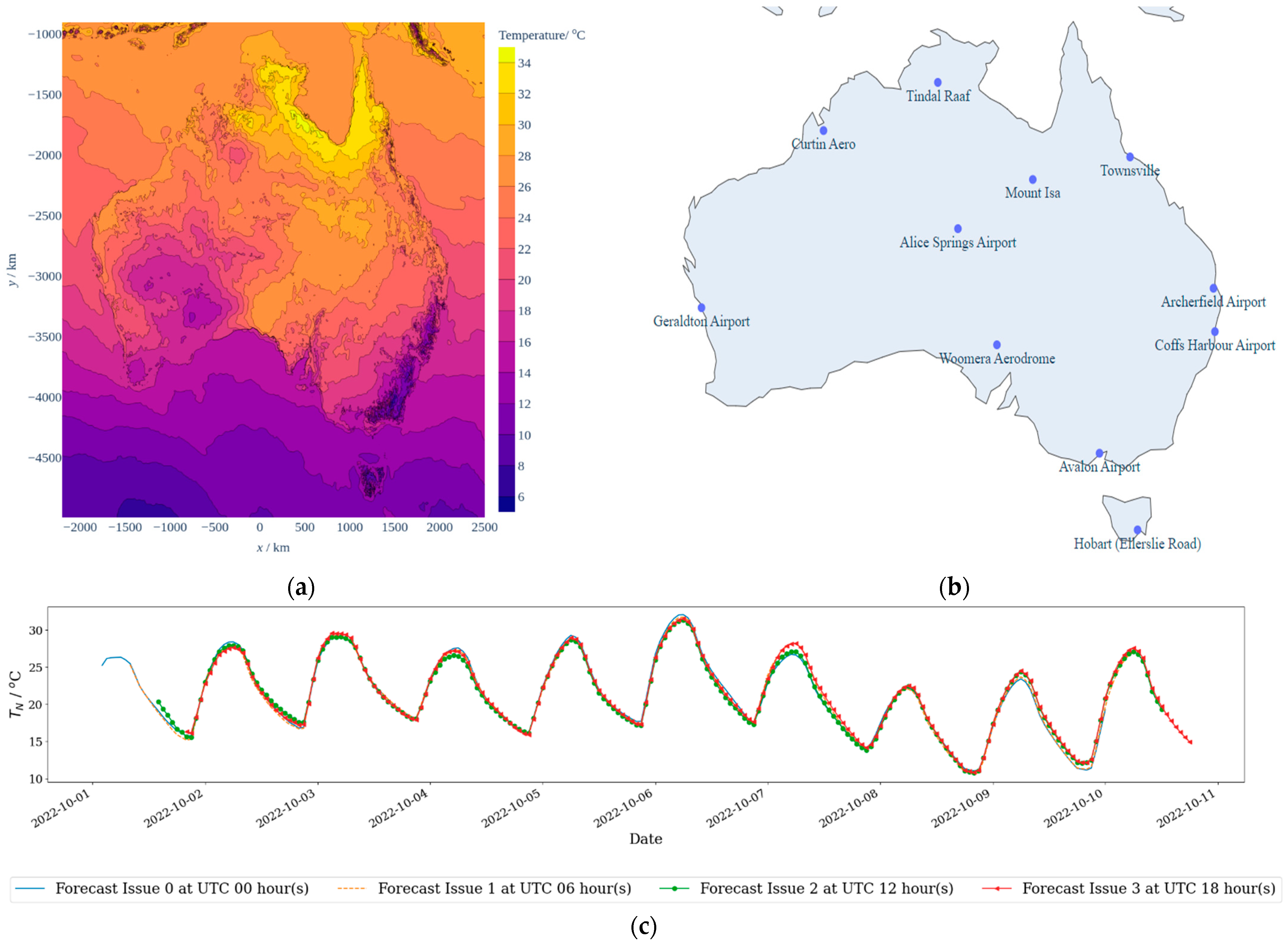
2. Data Overview
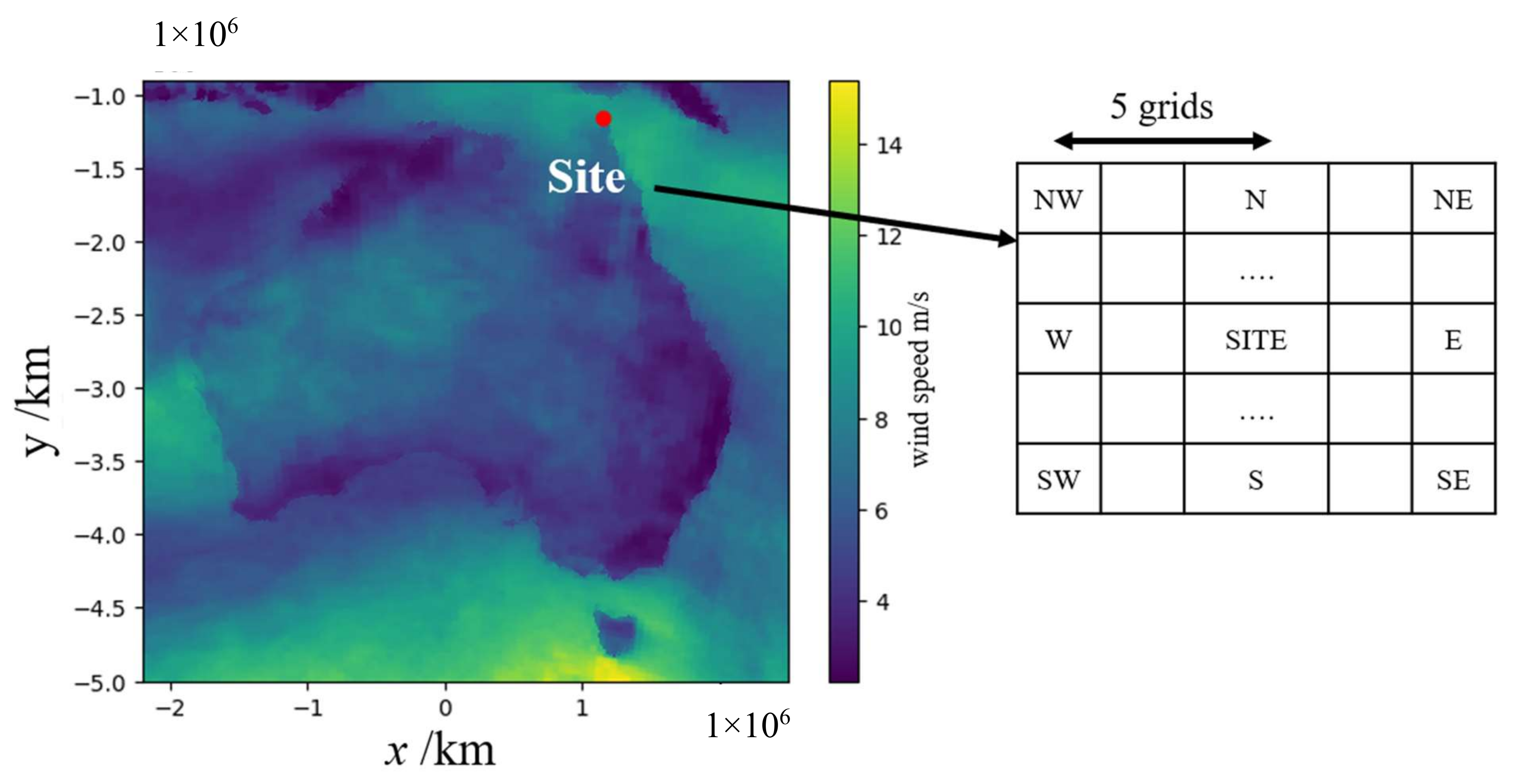
2.1. Gridded Numerical Data (IMPROVER)
2.2. Site Observations
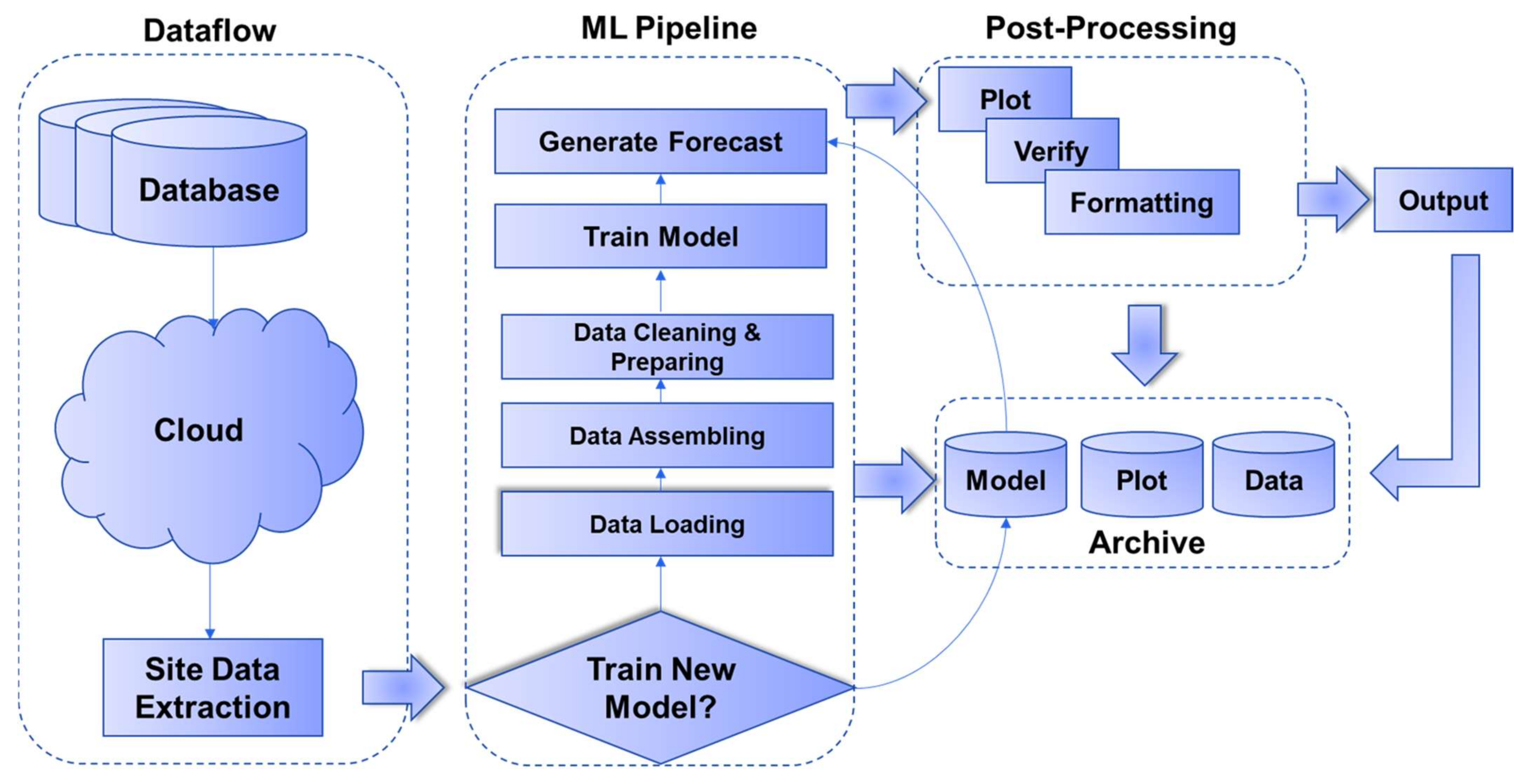
3. Model Training, Optimization and Explainability
3.1. Model Training and Optimization
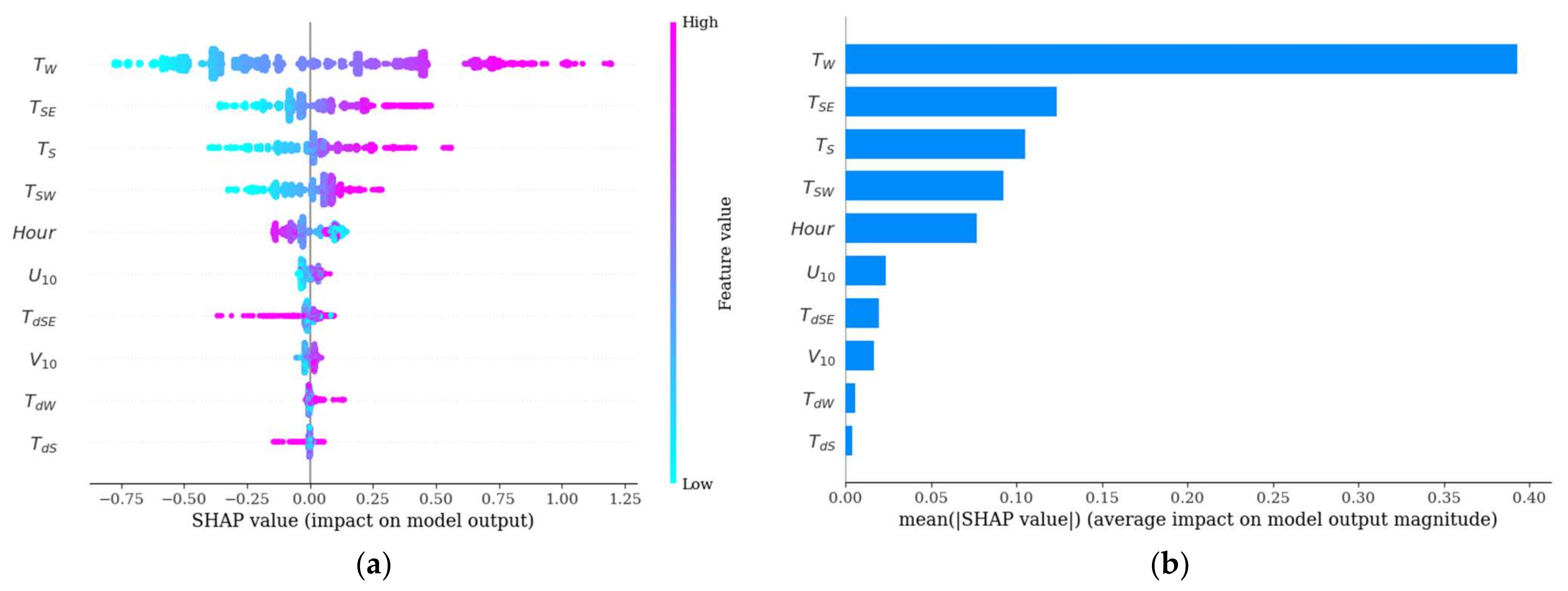
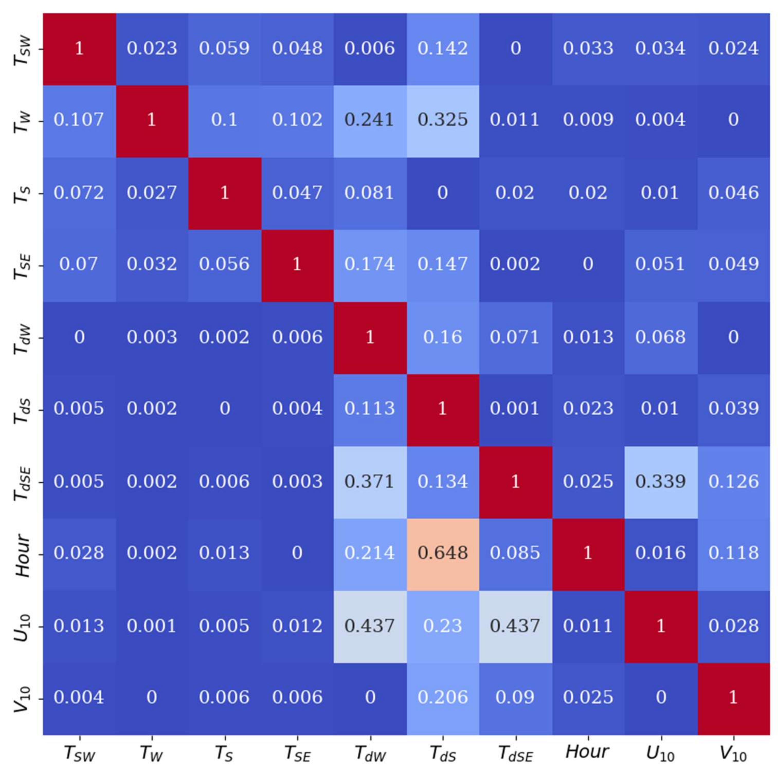
3.2. SHAP for ML Explainability
4. Experiments
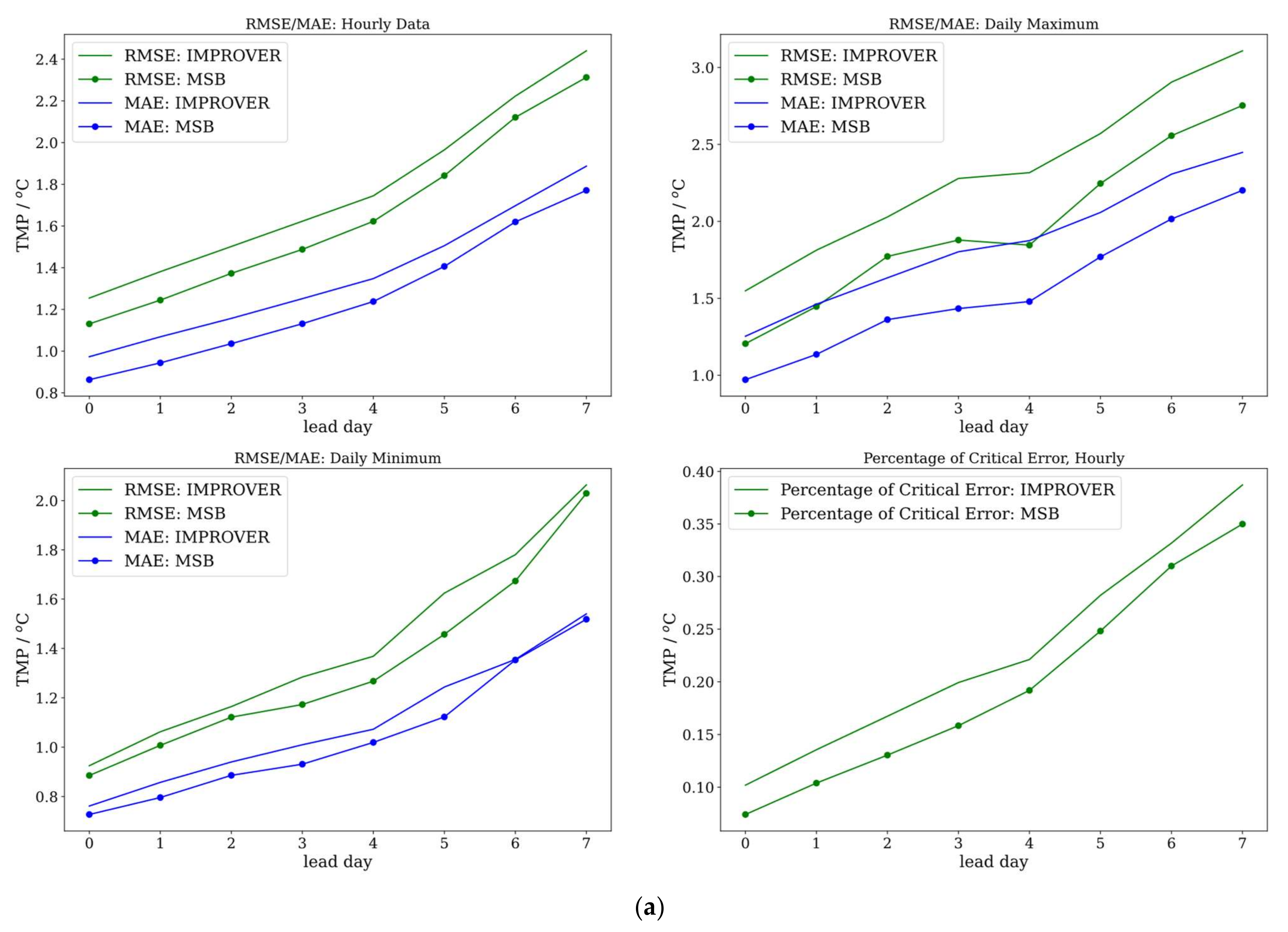
4.1. Evaluation Metrics
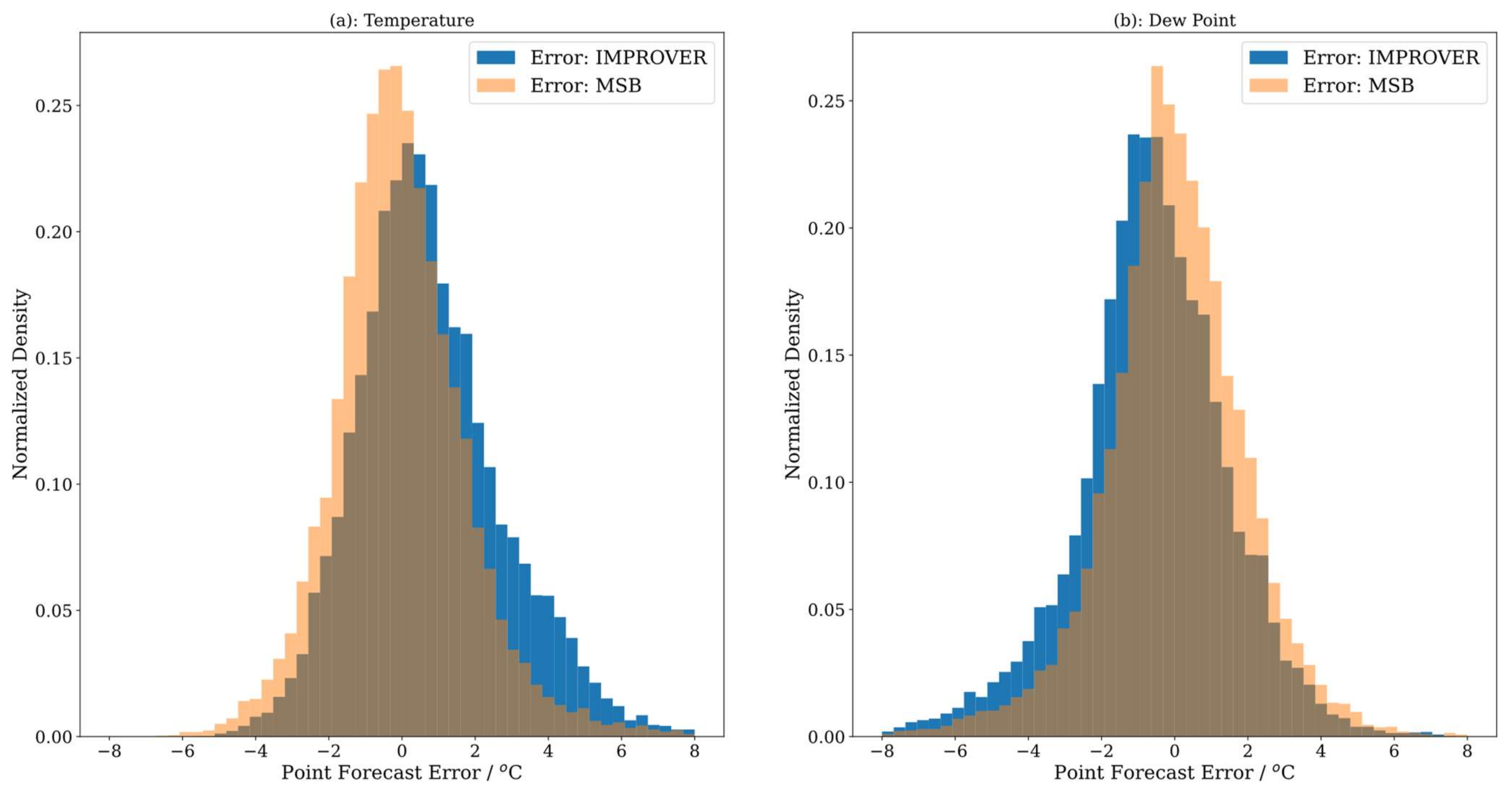
4.2. Results
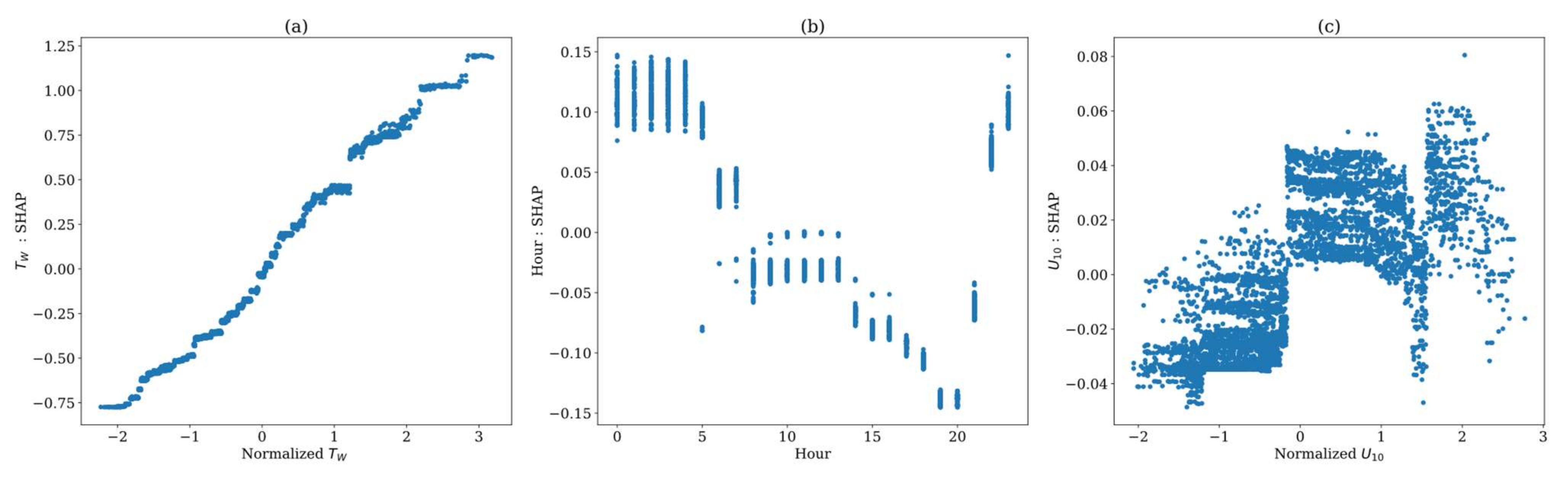
5. Explaining Model Outputs with SHAP
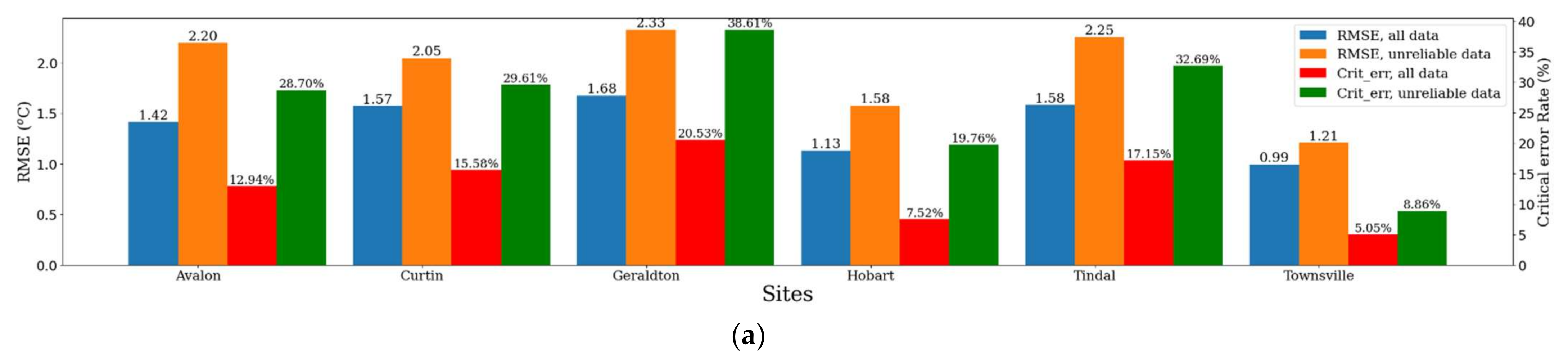
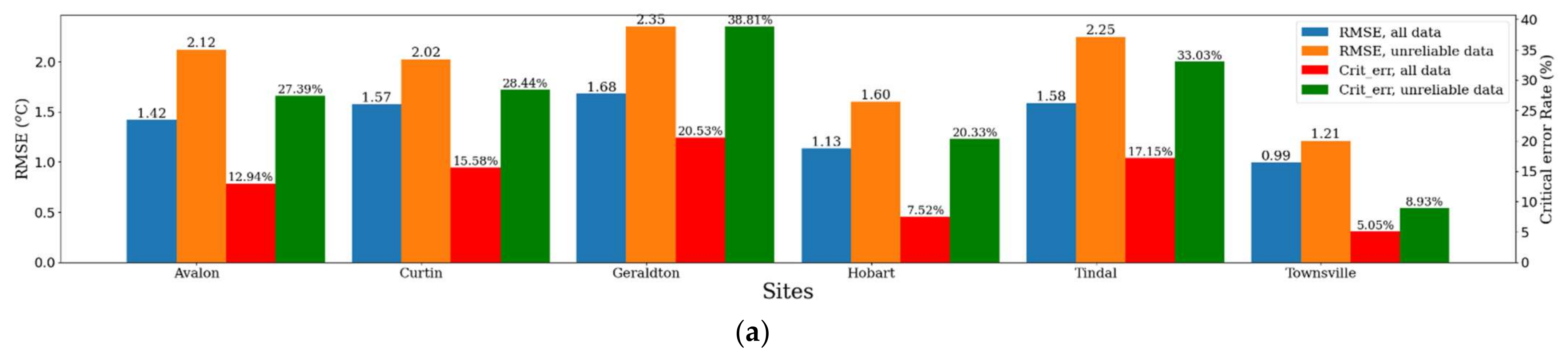
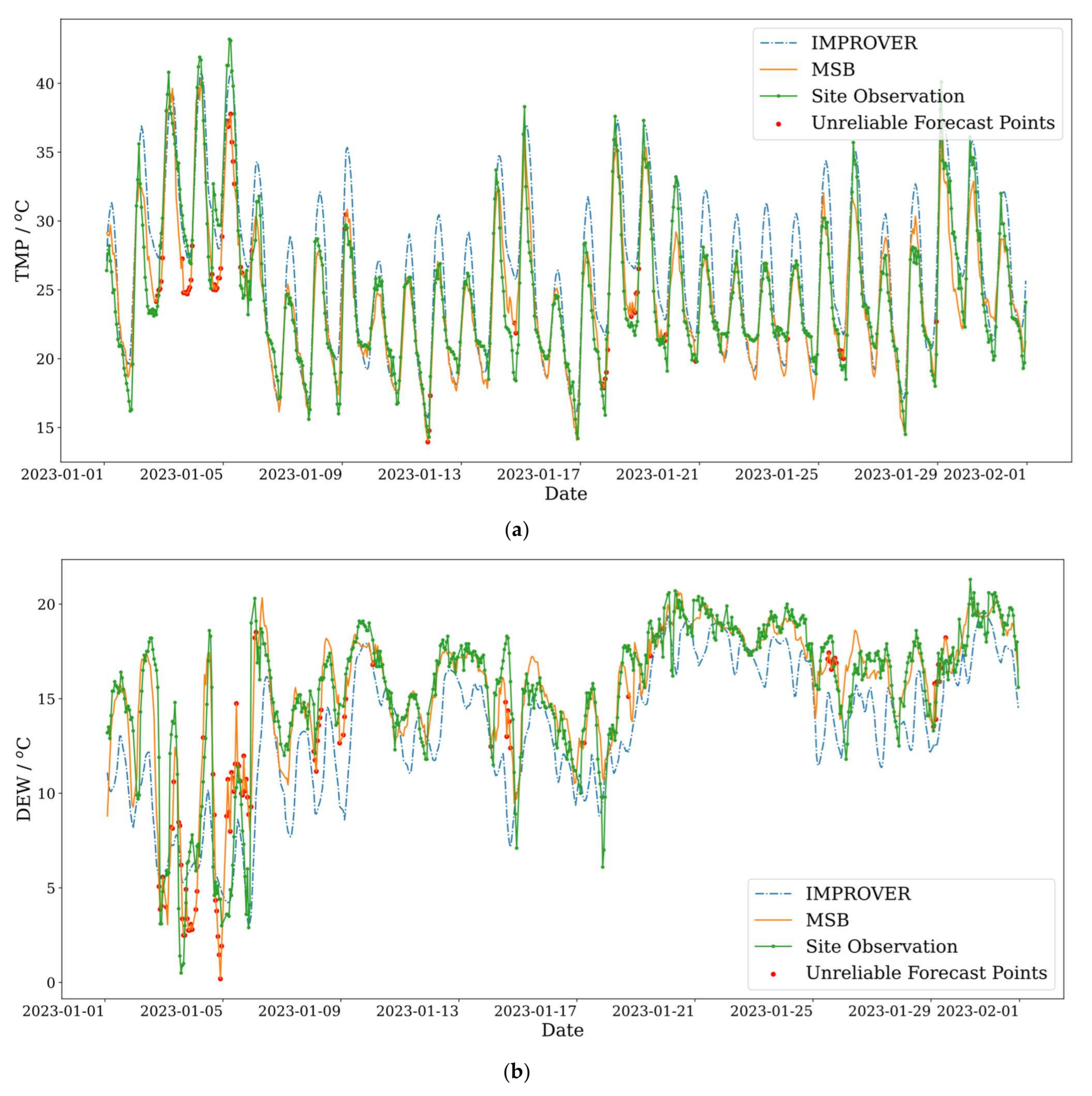
6. Error Analysis and Model Reliability
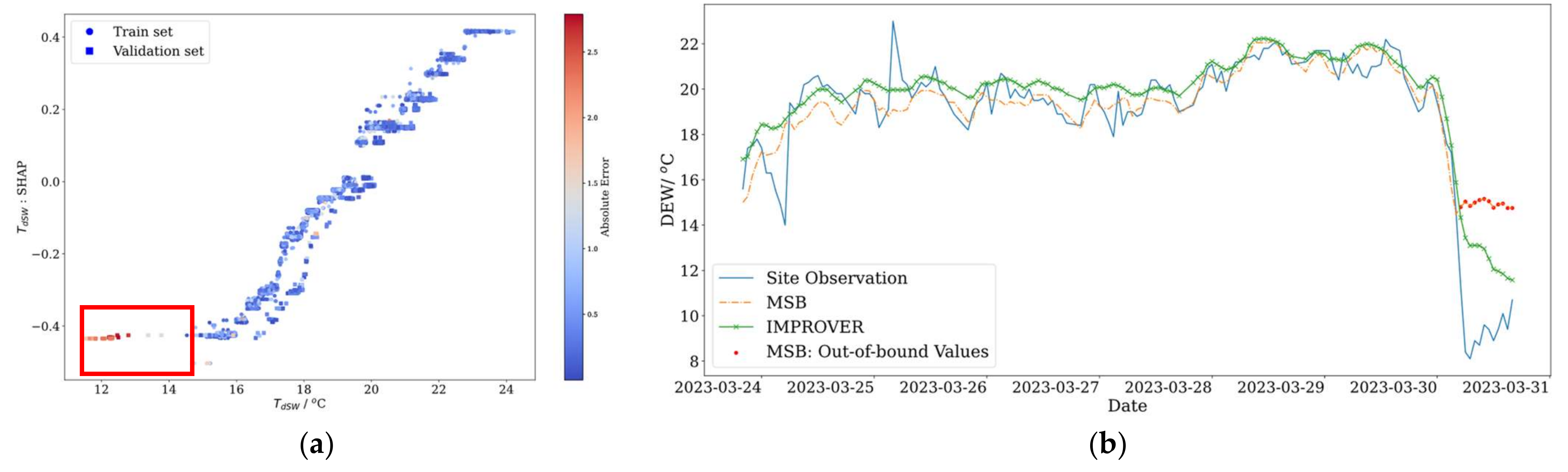
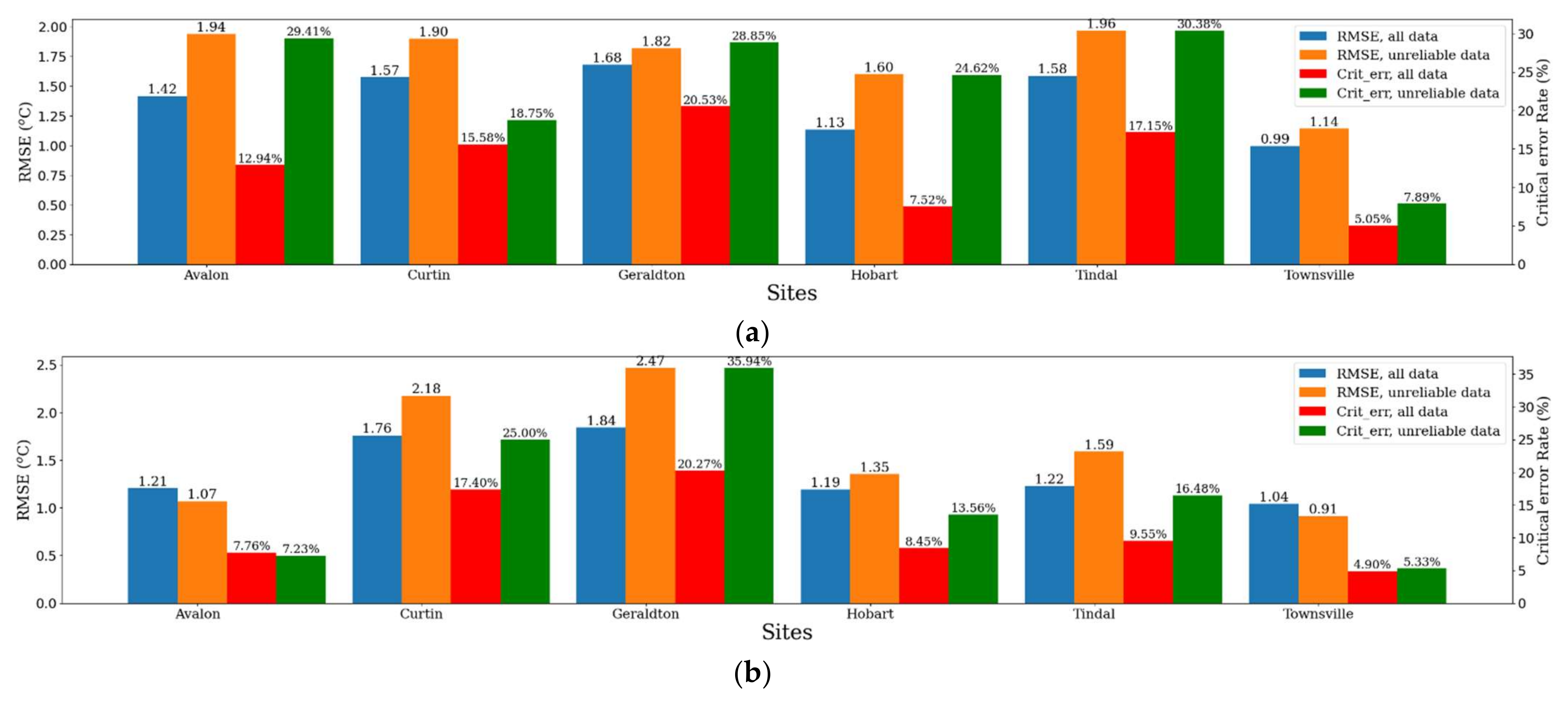
6.1. Unreliable Predictions from Out-of-Bound Feature Values
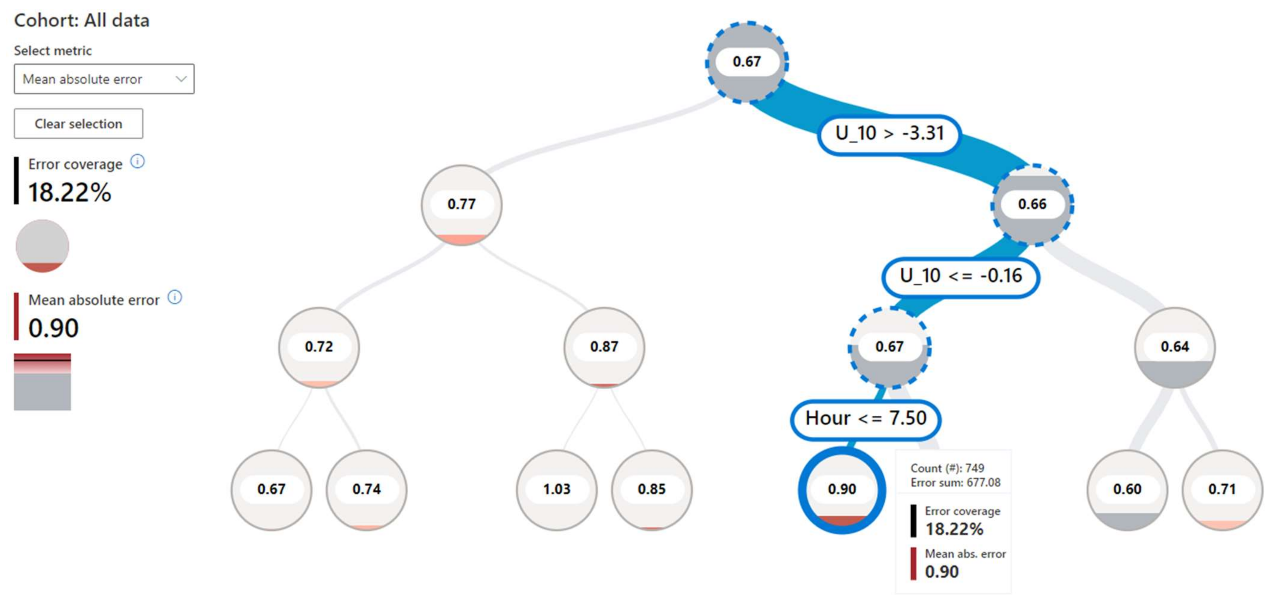
6.2. Unreliable Predictions in Poor-Performing Data Cohorts
6.3. Unreliable Predictions without Local Fit
6.4. Summary of Error Analysis and Model Reliability
7. Conclusions and Future Work
Author Contributions
Funding
Data Availability Statement
Conflicts of Interest
Appendix A

| Sites/Lead Time (Days) | 0 | 1 | 2 | 3 | 4 | 5 | 6 | 7 |
|---|---|---|---|---|---|---|---|---|
| Alice Springs Airport | −14.36 | −8.69 | 4.21 | 9.33 | 9.74 | 14.12 | 10.22 | 5.89 |
| Archerfield Airport | 33.62 | 33.97 | 33.27 | 29.04 | 29.46 | 29.15 | 32.26 | 35.17 |
| Avalon Airport | 10.93 | 15.30 | 3.91 | 6.71 | 8.90 | 10.39 | −0.41 | 5.42 |
| Coffs Harbour Airport | 22.37 | 27.60 | 29.31 | 26.34 | 27.11 | 24.10 | 21.25 | 22.37 |
| Curtin Aero | 17.42 | 12.30 | 12.19 | 13.58 | 21.83 | 20.00 | 22.42 | 18.33 |
| Geraldton Airport | 21.88 | 25.51 | 24.72 | 25.24 | 24.91 | 21.30 | 20.31 | 21.67 |
| Hobart (Ellerslie Road) | 22.17 | 20.20 | 12.63 | 17.57 | 20.33 | 12.64 | 11.98 | 11.43 |
| Mount Isa | 9.52 | 10.41 | 13.59 | 17.48 | 8.35 | 7.77 | 12.37 | 18.17 |
| Tindal RAAF | −0.99 | −1.40 | 5.52 | 13.70 | 19.09 | 18.51 | 8.23 | 9.39 |
| Townsville | 40.44 | 40.21 | 39.99 | 40.68 | 34.52 | 29.96 | 33.72 | 38.71 |
| Woomera Aerodrome | −14.59 | −13.44 | 0.64 | 6.44 | 6.66 | 11.21 | 5.13 | 7.93 |
| Site/Lead Time (Days) | 0 | 1 | 2 | 3 | 4 | 5 | 6 | 7 |
|---|---|---|---|---|---|---|---|---|
| Alice Springs Airport | 22.34 | 30.57 | 24.47 | 26.64 | 30.07 | 29.10 | 22.10 | 26.08 |
| Archerfield Airport | −22.87 | −24.99 | −21.63 | −13.30 | −16.71 | −6.05 | 3.43 | 4.45 |
| Avalon Airport | 10.76 | 17.61 | 19.01 | 16.96 | 21.53 | 19.75 | 17.86 | 21.69 |
| Coffs Harbour Airport | 11.97 | 11.58 | 10.07 | 14.37 | 12.35 | 14.26 | 18.65 | 17.65 |
| Curtin Aero | −4.10 | −0.74 | 5.55 | 11.45 | 12.07 | 11.54 | 14.79 | 13.29 |
| Geraldton Airport | 56.52 | 58.10 | 62.29 | 60.62 | 60.50 | 58.97 | 56.76 | 55.74 |
| Hobart (Ellerslie Road) | 8.77 | −5.70 | −2.54 | 0.98 | 2.58 | 1.53 | −8.63 | −6.81 |
| Mount Isa | −17.98 | −12.35 | −9.86 | −0.34 | 6.55 | 7.97 | 16.46 | 16.59 |
| Tindal RAAF | −8.02 | −14.47 | −9.09 | −6.19 | −2.40 | −4.88 | 5.70 | 4.93 |
| Townsville | 41.35 | 41.40 | 41.61 | 41.98 | 43.87 | 42.99 | 41.05 | 38.62 |
| Woomera Aerodrome | 2.22 | −0.21 | 1.63 | −0.62 | 2.67 | 9.03 | 5.14 | 7.87 |
| Site/Lead Time (Days) | 0 | 1 | 2 | 3 | 4 | 5 | 6 | 7 |
|---|---|---|---|---|---|---|---|---|
| Alice Springs Airport | 27.07 | 24.88 | 26.07 | 18.81 | 14.28 | 16.20 | 31.08 | 28.07 |
| Archerfield Airport | 28.32 | 22.11 | 23.56 | 22.77 | 24.67 | 23.85 | 24.89 | 21.16 |
| Avalon Airport | 16.67 | 12.56 | 13.00 | 17.94 | 14.91 | 17.68 | 19.25 | 13.74 |
| Coffs Harbour Airport | 33.92 | 32.81 | 36.97 | 32.35 | 34.03 | 33.46 | 34.86 | 37.92 |
| Curtin Aero | 9.45 | 10.37 | 14.83 | 11.45 | 12.66 | 14.54 | 19.71 | 23.85 |
| Geraldton Airport | 33.48 | 34.13 | 34.10 | 30.78 | 25.27 | 22.23 | 27.16 | 25.60 |
| Hobart (Ellerslie Road) | 4.28 | 5.19 | 3.68 | 8.67 | 7.37 | 10.29 | 6.01 | 1.66 |
| Mount Isa | 26.31 | 27.49 | 29.11 | 22.43 | 23.41 | 19.70 | 27.23 | 23.23 |
| Tindal RAAF | −0.58 | 2.67 | 8.03 | 11.79 | 5.07 | 5.06 | 24.70 | 21.63 |
| Townsville | 1.43 | 4.40 | 3.12 | 6.61 | 2.38 | 1.86 | 1.99 | 11.35 |
| Woomera Aerodrome | −10.90 | −6.77 | −4.91 | −10.26 | −11.21 | 2.01 | 3.22 | 0.93 |
| Site/Lead Time (Days) | 0 | 1 | 2 | 3 | 4 | 5 | 6 | 7 |
|---|---|---|---|---|---|---|---|---|
| Alice Springs Airport | −1.01 | −1.94 | 5.53 | 15.99 | 14.57 | 17.94 | 12.72 | 9.59 |
| Archerfield Airport | 47.64 | 42.17 | 39.90 | 41.47 | 38.15 | 34.59 | 35.87 | 35.91 |
| Avalon Airport | 3.84 | 9.68 | 9.57 | 12.27 | 14.82 | 13.42 | 5.51 | 6.76 |
| Coffs Harbour Airport | 13.62 | 12.14 | 18.29 | 19.17 | 15.54 | 19.32 | 17.73 | 19.63 |
| Curtin Aero | −3.98 | 1.22 | 4.51 | 7.58 | 8.47 | 8.37 | 6.47 | −0.52 |
| Geraldton Airport | 21.68 | 8.46 | 9.49 | 4.84 | 3.64 | 9.64 | 6.36 | 12.70 |
| Hobart (Ellerslie Road) | 20.57 | 21.22 | 21.69 | 19.79 | 22.14 | 23.02 | 16.99 | 16.53 |
| Mount Isa | 22.57 | 27.18 | 34.10 | 33.14 | 32.53 | 29.46 | 28.11 | 31.96 |
| Tindal RAAF | 24.14 | 21.34 | 20.64 | 30.12 | 20.13 | 19.69 | 16.34 | 14.90 |
| Townsville | −6.72 | −1.34 | −1.47 | 0.54 | 5.46 | 14.01 | 9.25 | −2.09 |
| Woomera Aerodrome | 34.81 | 30.51 | 33.03 | 34.27 | 33.56 | 30.85 | 30.09 | 28.04 |
| Site/Lead Time (Days) | 0 | 1 | 2 | 3 | 4 | 5 | 6 | 7 |
|---|---|---|---|---|---|---|---|---|
| Alice Springs Airport | 7.39 | 8.01 | 10.66 | 10.40 | 10.06 | 7.85 | 7.84 | 8.53 |
| Archerfield Airport | 3.91 | 4.50 | 6.15 | 6.01 | 6.90 | 7.87 | 8.94 | 8.42 |
| Avalon Airport | 1.32 | 1.25 | 1.46 | 1.27 | 2.73 | 2.06 | 2.25 | 2.11 |
| Coffs Harbour Airport | 5.37 | 6.18 | 6.86 | 6.60 | 6.63 | 5.64 | 5.03 | 5.16 |
| Curtin Aero | 0.82 | 0.89 | 1.07 | 2.57 | 2.59 | 3.32 | 4.31 | 6.08 |
| Geraldton Airport | 16.50 | 16.42 | 15.31 | 15.83 | 14.62 | 14.42 | 12.49 | 12.87 |
| Hobart (Ellerslie Road) | 2.78 | 3.16 | 3.69 | 4.09 | 2.93 | 3.39 | 2.18 | 3.72 |
| Mount Isa | 2.73 | 1.46 | 3.21 | 3.76 | 3.88 | 3.22 | 3.42 | 5.10 |
| Tindal RAAF | 3.81 | 4.62 | 4.68 | 5.92 | 5.93 | 4.97 | 6.49 | 6.96 |
| Townsville | 2.58 | 3.67 | 4.08 | 4.59 | 4.39 | 4.22 | 5.02 | 5.68 |
| Woomera Aerodrome | 1.41 | 3.07 | 4.09 | 5.23 | 5.92 | 5.96 | 4.40 | 7.13 |
| Site/Lead Time (Days) | 0 | 1 | 2 | 3 | 4 | 5 | 6 | 7 |
|---|---|---|---|---|---|---|---|---|
| Alice Springs Airport | 4.46 | 6.27 | 6.77 | 8.83 | 8.02 | 8.40 | 7.71 | 8.09 |
| Archerfield Airport | 8.29 | 8.03 | 7.04 | 8.29 | 8.10 | 8.75 | 8.52 | 6.70 |
| Avalon Airport | 1.20 | 1.55 | 0.72 | 1.25 | 2.30 | 2.29 | 2.03 | 2.54 |
| Coffs Harbour Airport | 0.95 | 0.54 | 0.90 | 0.81 | 0.85 | 2.07 | 4.42 | 5.02 |
| Curtin Aero | 0.42 | 1.16 | 1.47 | 0.98 | −0.06 | 1.51 | 1.14 | 2.23 |
| Geraldton Airport | 20.26 | 21.60 | 22.20 | 23.98 | 25.51 | 23.37 | 24.28 | 23.24 |
| Hobart (Ellerslie Road) | 1.44 | 2.25 | 2.73 | 2.44 | 4.34 | 4.52 | 4.73 | 4.70 |
| Mount Isa | 3.44 | 3.88 | 4.88 | 4.76 | 4.48 | 5.46 | 8.77 | 11.27 |
| Tindal RAAF | 0.64 | 2.10 | 3.08 | 2.93 | 2.95 | 2.73 | 1.06 | 0.74 |
| Townsville | 1.84 | 3.09 | 4.22 | 6.39 | 8.75 | 9.48 | 9.38 | 9.66 |
| Woomera Aerodrome | 9.02 | 10.50 | 9.72 | 8.48 | 5.76 | 4.53 | 4.60 | 3.66 |
References
- Vannitsem, S.; Bremnes, J.B.; Damaeyer, J.; Evans, G.R.; Flowerdew, J.; Hemri, S.; Lerch, S.; Roberts, N.; Theis, S.; Atencia, A.; et al. Statistical Postprocessing for Weather Forecasts: Review, Challenges, and Avenues in a Big Data World. Bull. Am. Meteorol. Soc. 2021, 102, E681–E699. [Google Scholar] [CrossRef]
- Richardson, D.S. Skill and relative economic value of the ECMWF ensemble prediction system. Q. J. R. Meteorol. Soc. 2000, 126, 649–667. [Google Scholar] [CrossRef]
- Bakker, K.; Whan, K.; Knap, W.; Schmeits, M. Comparison of statistical post-processing methods for probabilistic NWP forecasts of solar radiation. Sol. Energy 2019, 191, 138–150. [Google Scholar] [CrossRef]
- Yang, D. Post-processing of NWP forecasts using ground or satellite-derived data through kernel conditional density estimation. J. Renew. Sustain. Energy 2019, 11, 026101. [Google Scholar] [CrossRef]
- Alerskans, E.; Kaas, E. Local temperature forecasts based on statistical post-processing of numerical weather prediction data. Meteorol. Appl. 2021, 28, e2006. [Google Scholar] [CrossRef]
- Li, X.; Ma, L.; Chen, P.; Xu, H.; Xing, Q.; Yan, J.; Lu, S.; Fan, H.; Yang, L.; Cheng, Y. Probabilistic solar irradiance forecasting based on XGBoost. Energy Rep. 2022, 8, 1087–1095. [Google Scholar] [CrossRef]
- Karevan, Z.; Suykens, J.A. Transductive LSTM for time-series prediction: An application to weather forecasting. Neural Netw. 2020, 125, 1–9. [Google Scholar] [CrossRef]
- Kong, W.; Li, H.; Yu, C.; Xia, J.; Kang, Y.; Zhang, P. A deep spatio-temporal forecasting model for multi-site weather prediction post-processing. Commun. Comput. Phys. 2022, 31, 131–153. [Google Scholar] [CrossRef]
- Donadio, L.; Fang, J.; Porté-Agel, F. Numerical weather prediction and artificial neural network coupling for wind energy forecast. Energies 2021, 14, 338. [Google Scholar] [CrossRef]
- Hu, H.; van der Westhuysen, A.J.; Chu, P.; Fujisaki-Manome, A. Predicting Lake Erie wave heights and periods using XGBoost and LSTM. Ocean Model. 2021, 164, 101832. [Google Scholar] [CrossRef]
- Sushanth, K.; Mishra, A.; Mukhopadhyay, P.; Singh, R. Near-real-time forecasting of reservoir inflows using explainable machine learning and short-term weather forecasts. Stoch. Environ. Res. Risk Assess. 2023, 37, 3945–3965. [Google Scholar] [CrossRef]
- Chen, T.; He, T.; Benesty, M.; Khotilovich, V.; Tang, Y.; Cho, H.; Chen, K.; Mitchell, R.; Cano, I.; Zhou, T. Xgboost: Extreme Gradient Boosting. R package version 0.4-2 2015; Volume 1, pp. 1–4. Available online: https://pypi.org/project/xgboost/ (accessed on 16 July 2024).
- Grinsztajn, L.; Oyallon, E.; Varoquaux, G. Why do tree-based models still outperform deep learning on typical tabular data? Adv. Neural Inf. Process. Syst. 2022, 35, 507–520. [Google Scholar]
- Dong, J.; Zeng, W.; Wu, L.; Huang, J.; Gaiser, T.; Srivastava, A.K. Enhancing short-term forecasting of daily precipitation using numerical weather prediction bias correcting with XGBoost in different regions of China. Eng. Appl. Artif. Intell. 2023, 117, 105579. [Google Scholar] [CrossRef]
- Xiong, X.; Guo, X.; Zeng, P.; Zou, R.; Wang, X. A short-term wind power forecast method via XGBoost hyper-parameters optimization. Front. Energy Res. 2022, 10, 905155. [Google Scholar] [CrossRef]
- Zheng, H.; Wu, Y. A XGBoost model with weather similarity analysis and feature engineering for short-term wind power forecasting. Appl. Sci. 2019, 9, 3019. [Google Scholar] [CrossRef]
- Gunning, D.; Stefik, M.; Choi, J.; Miller, T.; Stumpf, S.; Yang, G.Z. XAI—Explainable artificial intelligence. Sci. Robot. 2019, 4, eaay7120. [Google Scholar] [CrossRef] [PubMed]
- Linardatos, P.; Papastefanopoulos, V.; Kotsiantis, S. Explainable AI: A review of machine learning interpretability methods. Entropy 2020, 23, 18. [Google Scholar] [CrossRef] [PubMed]
- Lundberg, S.M.; Lee, S.I. A unified approach to interpreting model predictions. In Proceedings of the 31st International Conference on Neural Information Processing Systems, Long Beach, CA, USA, 4–9 December 2017; Volume 30. [Google Scholar]
- Lundberg, S.M.; Erion, G.; Chen, H.; DeGrave, A.; Prutkin, J.M.; Nair, B.; Katz, R.; Himmelfarb, J.; Bansal, N.; Lee, S.-I. From local explanations to global understanding with explainable AI for trees. Nat. Mach. Intell. 2020, 2, 56–67. [Google Scholar] [CrossRef]
- Duckworth, C.; Chmiel, F.P.; Burns, D.K.; Zlatev, Z.D.; White, N.M.; Daniels, T.W.V.; Kiuber, M. Using explainable machine learning to characterise data drift and detect emergent health risks for emergency department admissions during COVID-19. Sci. Rep. 2021, 11, 23017. [Google Scholar] [CrossRef]
- Dikshit, A.; Pradhan, B. Explainable AI in drought forecasting. Mach. Learn. Appl. 2021, 6, 100192. [Google Scholar] [CrossRef]
- Dikshit, A.; Pradhan, B. Interpretable and explainable AI (XAI) model for spatial drought prediction. Sci. Total Environ. 2021, 801, 149797. [Google Scholar] [CrossRef] [PubMed]
- Zhang, X.; Chan, F.T.; Yan, C.; Bose, I. Towards risk-aware artificial intelligence and machine learning systems: An overview. Decis. Support Syst. 2022, 159, 113800. [Google Scholar] [CrossRef]
- Saria, S.; Subbaswamy, A. Tutorial: Safe and Reliable Machine Learning. arXiv 2019, arXiv:1904.07204. [Google Scholar] [CrossRef]
- Schulam, P.; Saria, S. Can you trust this prediction? Auditing pointwise reliability after learning. In Proceedings of the 22nd International Conference on Artificial Intelligence and Statistics, Naha, Japan, 16–18 April 2019; pp. 1022–1031. [Google Scholar]
- d’Eon, G.; d’Eon, J.; Wright, J.R.; Leyton-Brown, K. The spotlight: A general method for discovering systematic errors in deep learning models. In Proceedings of the 2022 ACM Conference on Fairness, Accountability, and Transparency, Seoul, Republic of Korea, 21–24 June 2022; pp. 1962–1981. [Google Scholar]
- Eyuboglu, S.; Varma, M.; Saab, K.; Delbrouck, J.; Lee-Messer, C.; Dunnmon, J.; Zou, J.; Re, C. Domino: Discovering Systematic Errors with Cross-Modal Embeddings. In Proceedings of the 2022 International Conference on Learning Representations, Online, 25–29 April 2022. [Google Scholar]
- Hellman, M.E. The nearest neighbor classification rule with a reject option. IEEE Trans. Syst. Sci. Cybern. 1970, 6, 179–185. [Google Scholar] [CrossRef]
- Roberts, N.; Ayliffe, B.; Evans, G.; Moseley, S.; Rust, F.; Sandford, C.; Trzeciak, T.; Abernethy, P.; Beard, L.; Crosswaite, N.; et al. IMPROVER: The New Probabilistic Postprocessing System at the Met Office. Bull. Am. Meteorol. Soc. 2023, 104, E680–E697. [Google Scholar] [CrossRef]
- Malistov, A.; Trushin, A. Gradient boosted trees with extrapolation. In Proceedings of the 2019 18th IEEE International Conference on Machine Learning and Applications (ICMLA), Boca Raton, FL, USA, 16–19 December 2019; IEEE: Piscataway, NJ, USA, 2019; pp. 783–789. [Google Scholar]
- Lundberg, S.M.; Erion, G.G.; Lee, S.I. Consistent individualized feature attribution for tree ensembles. arXiv 2018, arXiv:1802.03888. [Google Scholar]
- Delle Monache, L.; Nipen, T.; Liu, Y.; Roux, G.; Stull, R. Kalman filter and analog schemes to postprocess numerical weather predictions. Mon. Weather Rev. 2011, 139, 3554–3570. [Google Scholar] [CrossRef]
- Sheridan, P.; Vosper, S.; Smith, S. A physically based algorithm for downscaling temperature in complex terrain. J. Appl. Meteorol. Climatol. 2018, 57, 1907–1929. [Google Scholar] [CrossRef]
- Nori, H.; Jenkins, S.; Koch, P.; Caruana, R. InterpretML: A unified framework for machine learning interpretability. arXiv 2019, arXiv:1909.09223. [Google Scholar]


| Sites/Preprocessing Methods | Change of RMSE, If Feature Selection Is Not Performed | Change of RMSE, If Surrounding Points Are Excluded | Change of RMSE, If Scaling Is Not Performed |
|---|---|---|---|
| Alice Springs Airport | −0.01 | −0.09 | 0.50 |
| Archerfield Airport | 0.01 | 0.02 | 0.20 |
| Avalon Airport | 0.01 | −0.03 | 0.13 |
| Coffs Harbour Airport | 0.03 | 0.12 | 0.19 |
| Curtin Aero | 0.00 | 0.12 | 0.24 |
| Geraldton Airport | 0.01 | 0.19 | 0.09 |
| Hobart (Ellerslie Road) | −0.01 | 0.03 | 0.25 |
| Mount Isa | 0.01 | 0.04 | 0.68 |
| Tindal RAAF | −0.01 | −0.10 | 0.00 |
| Townsville | 0.02 | 0.09 | 0.28 |
| Woomera Aerodrome | −0.02 | −0.01 | 0.30 |
| SUM | 0.05 | 0.37 | 2.87 |
| AVERAGE | 0.005 | 0.034 | 0.261 |
| Site/Metrics | Hourly RMSE, MSB (Change from IMPROVER)/°C | Daily Maximum RMSE, MSB (Change from IMPROVER)/°C | Daily Minimum RMSE, MSB (Change from IMPROVER)/°C | Percentage of Critical Error, MSB (Change from IMPROVER)/% |
|---|---|---|---|---|
| Alice Springs Airport | 2.36 (−0.38) | 2.14 (−0.13) | 2.11 (−0.64) | 32.94% (−8.98%) |
| Archerfield Airport | 1.37 (−0.23) | 1.51 (−0.71) | 1.39 (−0.43) | 12.39% (−6.59%) |
| Avalon Airport | 1.92 (−0.07) | 2.11 (−0.14) | 1.77 (−0.34) | 23.50% (−1.31%) |
| Coffs Harbour Airport | 1.51 (−0.26) | 1.35 (−0.46) | 1.55 (−0.78) | 16.64% (−5.46%) |
| Curtin Aero | 1.79 (−0.13) | 1.67 (−0.33) | 1.33 (−0.24) | 20.60% (−2.73%) |
| Geraldton Airport | 2.09 (−0.60) | 2.22 (−0.68) | 2.09 (−0.87) | 29.67% (−13.45%) |
| Hobart (Ellerslie Road) | 1.64 (−0.12) | 1.95 (−0.37) | 1.34 (−0.06) | 19.53% (−3.30%) |
| Mount Isa | 2.19 (−0.21) | 1.96 (−0.25) | 2.00 (−0.56) | 31.95% (−2.63%) |
| Tindal RAAF | 1.82 (−0.16) | 1.57 (−0.14) | 1.38 (−0.15) | 22.70% (−5.34%) |
| Townsville | 1.13 (−0.20) | 0.99 (−0.60) | 1.15 (−0.04) | 7.44% (−4.39%) |
| Woomera Aerodrome | 1.93 (−0.11) | 1.83 (−0.04) | 1.75 (+0.07) | 21.44% (−4.28%) |
| Site/Metrics | Hourly RMSE, MSB (Change from IMPROVER)/°C | Daily Maximum RMSE, MSB (Change from IMPROVER)/°C | Daily Minimum RMSE, MSB (Change from IMPROVER)/°C | Percentage of Critical Error, MSB (Change from IMPROVER)/% |
|---|---|---|---|---|
| Alice Springs Airport | 2.67 (−0.46) | 2.40 (−0.88) | 2.66 (−0.30) | 38.55% (−7.40%) |
| Archerfield Airport | 1.73 (−0.41) | 1.46 (+0.13) | 2.02 (−1.29) | 17.25% (−7.96%) |
| Avalon Airport | 1.64 (−0.01) | 1.51 (−0.35) | 1.75 (−0.18) | 19.00% (−1.65%) |
| Coffs Harbour Airport | 1.43 (−0.16) | 1.36 (−0.19) | 1.82 (−0.34) | 11.99% (−2.11%) |
| Curtin Aero | 1.99 (−0.02) | 1.69 (−0.10) | 2.14 (−0.12) | 23.63% (−0.85%) |
| Geraldton Airport | 2.39 (−1.05) | 1.63 (−2.26) | 2.47 (−0.27) | 31.16% (−22.45%) |
| Hobart (Ellerslie Road) | 1.80 (−0.09) | 1.79 (+0.05) | 2.01 (−0.49) | 21.38% (−3.47%) |
| Mount Isa | 2.68 (−0.53) | 2.38 (−0.12) | 2.75 (−1.16) | 38.16% (−5.78%) |
| Tindal RAAF | 1.55 (−0.12) | 1.27 (0.06) | 1.83 (−0.49) | 14.73% (−2.17%) |
| Townsville | 1.34 (−0.29) | 1.10 (−0.80) | 2.01 (−0.11) | 9.24% (−6.57%) |
| Woomera Aerodrome | 2.49 (−0.35) | 2.17 (−0.11) | 2.30 (−1.07) | 34.54% (−7.15%) |
| Site/Lead Time (Days) | 0 | 1 | 2 | 3 | 4 | 5 | 6 | 7 |
|---|---|---|---|---|---|---|---|---|
| Alice Springs Airport | 15.27 | 13.66 | 14.38 | 14.67 | 13.93 | 13.94 | 13.29 | 12.07 |
| Archerfield Airport | 16.10 | 14.87 | 15.45 | 13.19 | 13.71 | 13.72 | 13.58 | 14.21 |
| Avalon Airport | 3.75 | 3.32 | 1.75 | 2.81 | 6.91 | 5.60 | 4.63 | 5.67 |
| Coffs Harbour Airport | 16.22 | 16.30 | 16.45 | 15.10 | 13.70 | 14.71 | 14.44 | 14.91 |
| Curtin Aero | 1.46 | 1.79 | 3.54 | 5.36 | 6.55 | 8.82 | 10.19 | 13.06 |
| Geraldton Airport | 27.58 | 27.36 | 26.12 | 24.16 | 22.44 | 21.98 | 21.40 | 21.23 |
| Hobart (Ellerslie Road) | 9.86 | 9.88 | 8.59 | 8.32 | 7.01 | 6.29 | 4.59 | 5.22 |
| Mount Isa | 8.78 | 7.69 | 8.68 | 8.76 | 9.28 | 10.22 | 13.64 | 14.14 |
| Tindal RAAF | 7.18 | 6.25 | 6.13 | 8.78 | 9.36 | 7.09 | 8.19 | 8.50 |
| Townsville | 15.54 | 17.45 | 17.29 | 16.64 | 12.91 | 12.52 | 12.37 | 15.18 |
| Woomera Aerodrome | 4.34 | 4.71 | 6.64 | 7.76 | 6.73 | 9.33 | 5.80 | 5.86 |
| Site/Lead Time (Days) | 0 | 1 | 2 | 3 | 4 | 5 | 6 | 7 |
|---|---|---|---|---|---|---|---|---|
| Alice Springs Airport | 10.70 | 11.74 | 15.30 | 17.89 | 18.30 | 14.66 | 12.89 | 13.30 |
| Archerfield Airport | 24.52 | 19.43 | 19.53 | 20.38 | 18.04 | 17.83 | 19.41 | 17.06 |
| Avalon Airport | 0.54 | 2.62 | 3.34 | 3.76 | 2.65 | 0.23 | −1.66 | −1.82 |
| Coffs Harbour Airport | 8.36 | 8.05 | 10.83 | 9.78 | 8.26 | 9.42 | 11.00 | 8.87 |
| Curtin Aero | −6.46 | −1.26 | 2.78 | 4.47 | 4.49 | 4.96 | 3.47 | 2.67 |
| Geraldton Airport | 37.13 | 33.37 | 31.56 | 30.58 | 30.59 | 30.50 | 29.48 | 28.14 |
| Hobart (Ellerslie Road) | 6.04 | 7.02 | 7.41 | 4.28 | 8.43 | 7.05 | 1.91 | −0.90 |
| Mount Isa | 4.62 | 8.64 | 14.55 | 18.51 | 18.44 | 16.60 | 19.67 | 21.49 |
| Tindal RAAF | 3.75 | 6.14 | 8.16 | 8.47 | 7.93 | 9.46 | 6.42 | 7.24 |
| Townsville | 10.61 | 11.57 | 14.16 | 15.77 | 22.43 | 24.06 | 19.77 | 14.35 |
| Woomera Aerodrome | 16.97 | 15.90 | 14.78 | 13.49 | 14.15 | 11.24 | 10.57 | 7.88 |
Disclaimer/Publisher’s Note: The statements, opinions and data contained in all publications are solely those of the individual author(s) and contributor(s) and not of MDPI and/or the editor(s). MDPI and/or the editor(s) disclaim responsibility for any injury to people or property resulting from any ideas, methods, instructions or products referred to in the content. |
© 2024 by the authors. Licensee MDPI, Basel, Switzerland. This article is an open access article distributed under the terms and conditions of the Creative Commons Attribution (CC BY) license (https://creativecommons.org/licenses/by/4.0/).
Share and Cite
Han, M.; Leeuwenburg, T.; Murphy, B. Site-Specific Deterministic Temperature and Dew Point Forecasts with Explainable and Reliable Machine Learning. Appl. Sci. 2024, 14, 6314. https://doi.org/10.3390/app14146314
Han M, Leeuwenburg T, Murphy B. Site-Specific Deterministic Temperature and Dew Point Forecasts with Explainable and Reliable Machine Learning. Applied Sciences. 2024; 14(14):6314. https://doi.org/10.3390/app14146314
Chicago/Turabian StyleHan, Mengmeng, Tennessee Leeuwenburg, and Brad Murphy. 2024. "Site-Specific Deterministic Temperature and Dew Point Forecasts with Explainable and Reliable Machine Learning" Applied Sciences 14, no. 14: 6314. https://doi.org/10.3390/app14146314
APA StyleHan, M., Leeuwenburg, T., & Murphy, B. (2024). Site-Specific Deterministic Temperature and Dew Point Forecasts with Explainable and Reliable Machine Learning. Applied Sciences, 14(14), 6314. https://doi.org/10.3390/app14146314