Adaptive Mask-Based Interpretable Convolutional Neural Network (AMI-CNN) for Modulation Format Identification

Abstract

Recently, various deep learning methods have been applied to Modulation Format Identification (MFI). The interpretability of deep learning models is important. However, this interpretability is challenged due to the black-box nature of deep learning. To deal with this difficulty, we propose an Adaptive Mask-Based Interpretable Convolutional Neural Network (AMI-CNN) that utilizes a mask structure for feature selection during neural network training and feeds the selected features into the classifier for decision making. During training, the masks are updated dynamically with parameters to optimize feature selection. The extracted mask serves as interpretable weights, with each weight corresponding to a feature, reflecting the contribution of each feature to the model’s decision. We validate the model on two datasets—Power Spectral Density (PSD) and constellation phase histogram—and compare it with three classical interpretable methods: Gradient-Weighted Class Activation Mapping (Grad-CAM), Local Interpretable Model-Agnostic Explanations (LIME), and Shapley Additive exPlanations (SHAP). The MSE values are as follows: AMI-CNN achieves the lowest MSE of 0.0246, followed by SHAP with 0.0547, LIME with 0.0775, and Grad-CAM with 0.1995. Additionally, AMI-CNN achieves the highest PG-Acc of 1, whether on PSD or on constellation phase histogram. Experimental results demonstrate that the AMI-CNN model outperforms compared methods in both qualitative and quantitative analyses.

1. Introduction

With the explosive growth of human demand for communication, optical network architectures are becoming dynamic, complex, and transparent [1]. In this context, elastic optical networks (EONs) must dynamically adjust the modulation format used for encoding optical signals based on varying channel characteristics and diverse data services. This requirement poses new challenges for digital coherent receivers [2]. Therefore, embedding an MFI module in digital coherent receivers is of significant importance, as it enables real-time identification of the modulation format of incoming signals [3].

In recent years, various machine learning methods have been applied to MFI. However, due to their limitations in feature processing, deep learning has emerged as the mainstream approach with advancing technology. The existing literature [4,5,6,7,8,9,10,11,12] focuses on improving various performance metrics of deep learning models, such as accuracy, robustness, speed, and efficiency. Although these metrics have seen certain improvements, relatively few studies have focused on the interpretability of deep learning models.

Due to the black-box nature of deep learning, the identification results are difficult to explain. The goal of Explainable Artificial Intelligence (XAI) is to design and implement AI systems that can produce accurate predictions or decisions and provide interpretable explanations for their outputs [13]. By showing the underlying reasoning and decision-making processes of models, XAI enables users to validate, control, improve, and gain insights into the model’s behavior [14]. In the complex and extensive EONs, practitioners may be familiar with optical networks but may not fully comprehend the internal algorithms of learning models. By combining optical theory with learning algorithms, practitioners can gain a better understanding of the learning model, facilitating subsequent maintenance and optimization.

To enhance the interpretability of models in MFI, Ref. [15] introduces a method utilizing multi-head attention mechanisms. This method enhances model interpretability by adjusting the internal structure of the model and visualizing the weights of each attention head, clearly presenting the decision-making process and key focus areas through heatmaps. However, due to the complex structure of multi-head attention mechanisms, this approach inevitably increases computational resource consumption and extends both training time and runtime.

In addition, Yin et al. [16] abandon high-complexity attention mechanisms in favor of the model-agnostic Grad-CAM method. They utilize Grad-CAM to generate heatmaps by computing gradient information from the final convolutional layer of a convolutional neural network. The gradient illustrates the focus areas of the model for each modulation format. This method intuitively shows the most critical regions in the input image, aiding in the understanding of the model’s decision rationale. However, the Grad-CAM method, while not adding to the complexity of the model itself, requires complex gradient computations after the model training to generate heatmaps.

Additionally, these studies primarily involve qualitative analysis, lacking quantitative measurement support. For instance, the color intensity of the heatmap only provides relative information about the model’s focus areas and cannot precisely quantify the effectiveness of each interpretability method.

To address these challenges, we introduce an Adaptive Mask-Based Interpretable Convolutional Neural Network (AMI-CNN). Our model improves discriminative capability and interpretability by using adaptive masks to highlight relevant features and suppress irrelevant ones. During training, the masks are updated dynamically with parameter adjustments to optimize feature selection. Despite enhancing interpretability through internal adjustments, AMI-CNN remains simple, with significantly fewer parameters than attention mechanisms. Unlike Grad-CAM, AMI-CNN shows interpretability directly through the weights of the masks, without the need for additional gradient computations. In addition to qualitative analysis, we employed Mean Squared Error (MSE) and the localization-based metric pointing game accuracy (PG-Acc) for quantitative analysis. Qualitative analysis of two datasets shows that AMI-CNN has superior interpretability.

The main contributions of this paper are two-fold, which are as follows:

(1)

This paper proposes an Adaptive Mask-Based Interpretable Convolutional Neural Network (AMI-CNN) for MFI. The model improves discriminative capability and interpretability by using adaptive masks to highlight relevant features and suppress irrelevant ones. Furthermore, adaptive masks automatically adjust during model training, and can directly interpret features after training without additional interpretative techniques.

(2)

We propose two metrics to evaluate the performance of the model interpretability. To our knowledge, in modulation format recognition, existing interpretability evaluations primarily rely on qualitative analysis alone. Our study employs quantitative metrics to provide a more accurate assessment of model interpretability.

2. Background and Literature Review

2.1. MFI

In recent years, various machine learning methods have been applied to the field of Modulation Format Identification, including Random Forests [17], Support Vector Machines [18,19], and several Artificial Neural Networks (ANNs) [20,21,22,23]. However, these machine learning algorithms exhibit limitations in feature processing capabilities and often underperform when handling complex tasks. With the increasing demand for high-speed transmission in communication systems, traditional MFI techniques have become inadequate to meet current requirements [24].

Consequently, deep learning (DL) methods have emerged as powerful alternatives. These methods have significantly improved the performance metrics of MFI in practical applications. In the literature [4,5,6,7,8], researchers have employed features such as one-dimensional amplitude histograms, constellations, eye diagrams, asynchronous amplitude histograms, and amplitude histograms in combination with deep learning networks to achieve high accuracy in commonly used modulation formats like MPSK and MQAM. The study in [9] proposed an Elastic Convolutional Neural Network (ElsNet), which enhances model robustness by optimizing internal parameters and dynamically adjusting the connections between network neurons. In Ref. [10], the authors introduced a few-shot learning algorithm by incorporating auxiliary tasks into Model-Agnostic Meta-Learning (MAML), allowing the gradient of meta-tasks to descend more quickly in the optimal target direction, thereby accelerating the model. Furthermore, Refs. [11,12] proposed multi-task models that can simultaneously handle tasks such as MFI and OSNR, improving efficiency while using additional tasks to constrain the accuracy of MFI, thus enhancing the efficiency and effectiveness of MFI systems.

Despite significant improvements in accuracy, robustness, speed, and efficiency, research on interpretability remains relatively limited.

2.2. Explainable Artificial Intelligence

The primary objective of Explainable Artificial Intelligence (XAI) is to provide descriptive insights into machine learning models, enabling justification, control, improvement, and discovery [14]. Due to the increasing complexity and widespread adoption of deep learning models, the demand for interpretability has received significant attention [25]. It is crucial to unlock the black box of AI and demonstrate its reliability, robustness, and interpretability [26]. XAI [27,28] has become an important area of AI research and development.

In Ref. [27], interpretable techniques are categorized into two main types: model-based explanation and post hoc explanation. Model-based explanations focus on the creation of interpretable models, while post hoc explanations aim to describe black-box models [13]. Interpretable models refer to linear regression [29] or decision tree [30], while typical black-box models are deep learning [31].

For black-box models, we primarily rely on other interpretable techniques for post hoc explanations. Common methods such as LIME [32] and SHAP [33] are applicable across various machine learning models. LIME utilizes linear approximation to construct interpretable surrogate models for explaining individual predictions, although these surrogate models may not always be accurate. On the other hand, SHAP, grounded in Shapley value theory, offers robust measures of feature contributions suitable for local and global explanations, albeit with high computational complexity. With the advancement of deep learning, researchers have proposed additional interpretable techniques tailored to deep learning models. Common interpretable methods are mainly applied to the image domain, such as occlusion maps, salience maps, class activation maps, and attention maps [34,35,36]. Based on these techniques, a variety of interpretable model variants have been developed, such as Grad-CAM [37]. This method generates highlighted regions in images that correspond to specific categories by using gradient information from convolutional neural networks. It can also be extended to one-dimensional models. However, it often emphasizes large areas and may overlook local details, which can affect the precision and sensitivity of localizing small targets.

Table 1. Comparison of common interpretability techniques.

Technique	Explanation Scope	Computational Complexity	Theoretical Basis	Limitation
LIME	Local	Moderate	Linear approximation	Depends on the surrogate model
SHAP	Global and local	High	Shapley values (cooperative game theory)	Requires complex calculations
Grad-CAM	Local	Moderate	Gradient computation	Can be less precise for small object localization

provides a comparative analysis of three classical models based on explanation scope, computational complexity, theoretical basis, and limitations.

In summary, we require an interpretable method that is free from surrogate model construction, has low computational complexity, and effectively handles detail features. This paper proposes a method to achieve these goals by introducing adaptive masks. Adaptive masks directly operate on earlier convolutional layers with more features to ensure the processing of detail features. Importantly, the feature weights represented by adaptive masks are obtained automatically as the model trains, eliminating the need for surrogate model construction and complex subsequent computations.

3. Materials and Methods

3.1. Experimental System

We set up the experimental system based on VPI Transmission Maker 9.0 to generate three widely used optical signals (QPSK, 8PSK, 16QAM) modulated at 10G baud in Figure 1. At the transmitter terminal, a pseudo-random binary sequence (PRBS) is mapped into MQAM and MPSK signals. The system utilizes a continuous wave (CW) laser with a center frequency of 193.1 THz, a linewidth of 0.1 MHz, and a power of 10 dBm to generate the optical carrier signal. It is used to drive a dual Mach–Zehnder modulator (dual MZM). The modulated signal is transmitted through a standard single-mode fiber (SSMF) extending by 1 km, characterized by an attenuation of 0.2 dB/km. At the optical receiving terminal, the optical signal was subsequently converted into an electrical signal. The local oscillator (LO) operates at a wavelength of 1550 nm with a linewidth of 0.1 kHz. It is mixed with the transmitted optical signal, and a demodulated signal is generated using a 90-degree Optical Hybrid. Subsequently, a photodetector is employed to convert the optical signal into an electrical signal. Following synchronized sampling by two analog-to-digital converters (ADC), two digital signals encapsulating in-phase (I) and quadrature (Q) information are acquired. These signals are processed using an offline DSP module to extract the two required datasets: PSD and constellation phase histogram.

3.2. Dataset Collection and Preprocessing

3.2.1. PSD Dataset

PSD offers insights into the frequency components of a signal and their power distribution across various frequencies. Due to the varying power distribution characteristics among different modulation formats, and its ease of acquisition, we can utilize PSD as a feature for identifying modulation formats. In this study, we subject the extracted I/Q signal $x\left[n\right]=I\left[n\right]+jQ\left[n\right]$ to the Fourier transform, compute the power spectrum at each frequency point, and ultimately normalize it to obtain PSD. The formula is as follows:

$$PSD\left[n\right]={\displaystyle \frac{1}{N}}{\left|DFT\left(x\left[n\right]\right)\right|}^2, n=0, 1, 2\cdots N-1$$

(1)

In our system, we select OSNR ranging from 15 to 26 dB in 1 dB increments and chromatic dispersion (CD) values ranging from −100 to 100 ps/nm in 10 ps/nm increments for each modulation format. This yields a total of 252 (12 × 21) combinations of OSNR and dispersion values. To ensure diversity within the dataset, we generate data using 10 distinct random seeds for each combination, resulting in 2520 samples per modulation format. Overall, we collect 7560 data samples across the three modulation formats. From this dataset, we allocate 180 samples to the test set, while dividing the remaining samples into a validation set (30%) and a training set (70%). The PSD dataset is considered a one-dimensional input for the deep learning network. Figure 2 presents the results from visualizing a subset of the data.

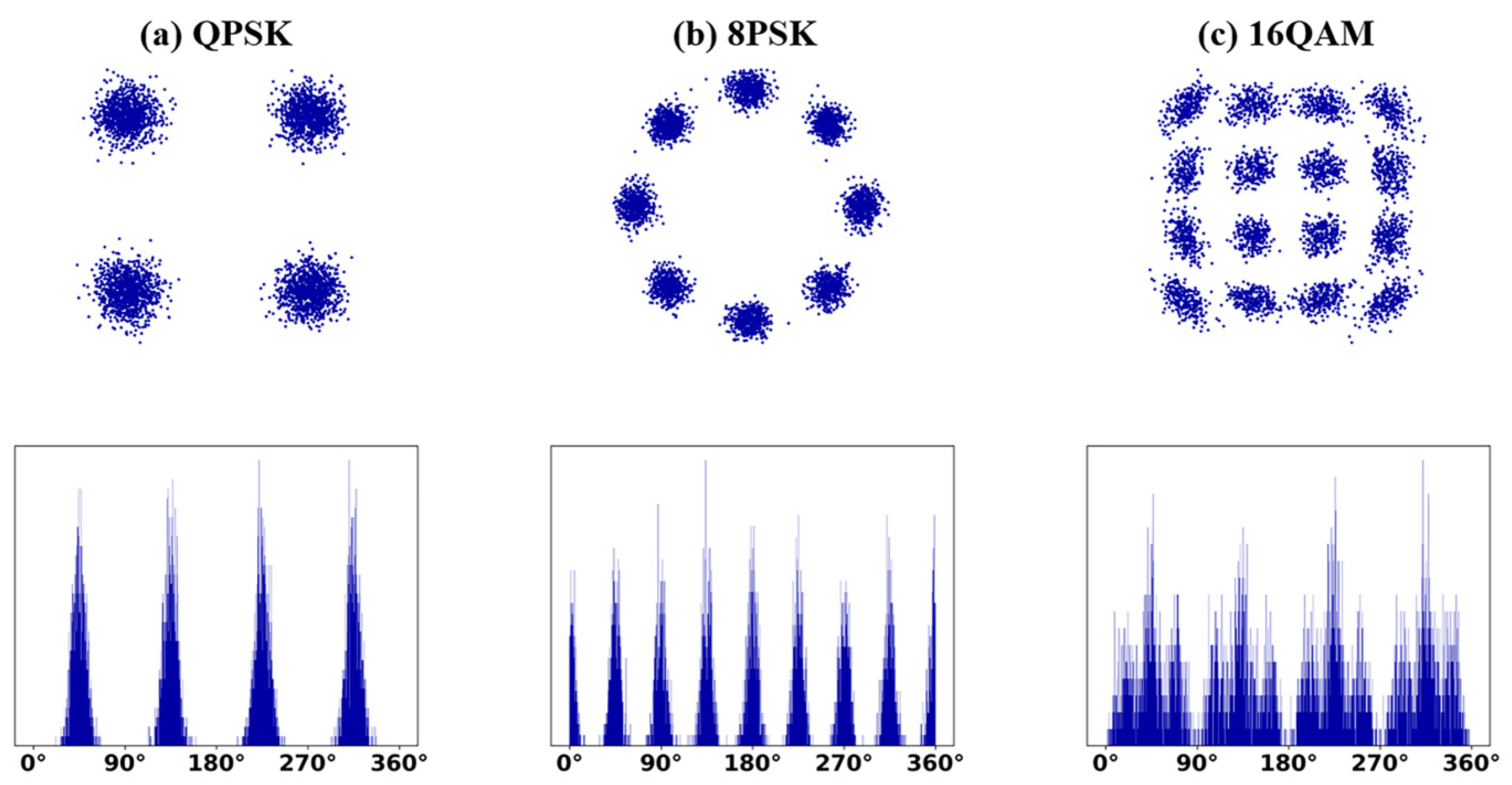
3.2.2. Constellation Phase Histogram Dataset

The literature [16] indicates that distinct modulation formats result in the constellation diagram displaying varying shape characteristics. Therefore, the distribution characteristics of clustered points in constellation diagrams serve as features for modulation format recognition, a widely utilized approach documented in numerous studies [5,16]. After receiving the I/Q signal, the constellation diagram is created by plotting the real $I$ as the horizontal coordinate and the imaginary $Q$ as the vertical coordinate of each sampling point. However, in this paper, we have introduced an offline processing module to reprocess the constellation diagram and extract its phase histogram as the dataset.

In the offline processing module, we use the I/Q signal to obtain the phase histogram as follows. For each data point $(I_i,Q_i)$, the phase is calculated as

$$\mathrm{\varnothing }=\arctan \left({\displaystyle \frac{Q_i}{I_i}}\right)$$

(2)

where $I_i$ is the real part of the data point and $Q_i$ is the imaginary part of the data point. Subsequently, the phase is divided into 1024 intervals, each with a width of $∆\mathrm{\varnothing }=2\pi /1024$. Thus, the phase range of the $k$-th interval is

$$\left[{\mathrm{\varnothing }}_{\mathit{k}},{\mathrm{\varnothing }}_{\mathit{k}}+∆\mathrm{\varnothing }\right]$$

(3)

where $k=\mathrm{0,1},2,\cdots ,1023$. For each data point $(I_i,Q_i)$, if its phase ${\mathrm{\varnothing }}_i$ falls within the k-th interval, the frequency $f_k$ of the phase interval is incremented by 1. Thus, the frequency $f_k$ of k within the interval is calculated as

$$f_k=f_k+1$$

(4)

Eventually, by traversing all the data points and accumulating the frequencies, the frequency information within each interval can be obtained, thereby forming a phase histogram. Figure 3 depicts the constellation diagrams and the corresponding phase histograms for each modulation format.

This paper investigates the phase histograms of three primary modulation formats (QPSK/8PSK/16QAM). These modulation formats span OSNR values ranging from 19 to 30 dB, with increments of 1 dB, and CD values ranging from −100 to 100 ps/nm, with increments of 10 ps/nm. Each combination is replicated with 10 different random seed counts, resulting in a total dataset of 7560 samples (3 × 12 × 21 × 10). Subsequently, 180 samples are designated as the test set, while the remaining data are randomly partitioned into training and validation sets in a 7:3 ratio.

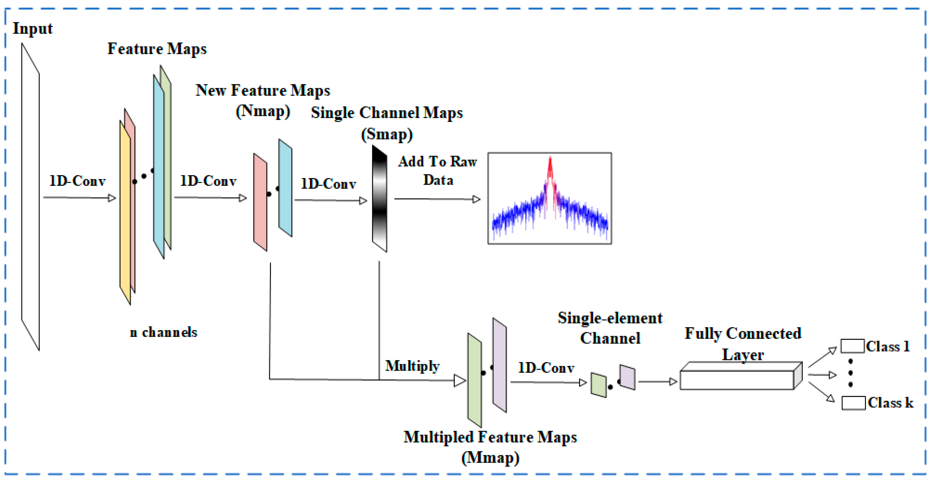
3.3. AMI-CNN Model Structure

The AMI-CNN model comprises three components: feature extraction, adaptive mask, and classifier. Figure 4 depicts the schematic architecture of the AMI-CNN model. Additionally, this section introduces the methodology for interpretability analysis using the mask, thereby facilitating a deeper understanding of the AMI-CNN model’s decision-making process.

3.3.1. Feature Extraction

The primary function of the feature extraction module is to expand the number of channels of the input features through convolution operations. Thereafter, these features are reorganized to obtain superior features. The specific operations are as follows.

In the AMI-CNN model, the network performs convolution operations on the input data using 5-sized convolutional kernels to extract rich multi-channel feature information, known as Feature Maps. This process results in the compression of spatial dimensions and an increase in the number of channels. Subsequently, the Feature Maps undergo downsampling through pooling layers to merge semantically similar features and reduce the dimensionality of the Feature Maps while retaining their essential semantic information. During this process, activation functions are introduced to introduce non-linear factors and enhance the model’s expressive power. The specific formula is as follows:

$$ReLU\left(x\right)=\left\{\begin{array}{c}x,if x\ge 0\\ 0,else\end{array}\right.$$

(5)

Subsequently, the model begins to reorganize the channel features while compressing the spatial dimensions. The model employs one-dimensional convolution with a kernel size of 5 and a stride of 1 to perform multiple operations on the Feature Maps to obtain $N_{map}$. This operation not only helps compress the length of the Feature Maps but also reduces the number of channels, further refining and extracting crucial features. Through this process of channel feature reorganization, the model can better capture key information in the data and provide more representative feature representations for subsequent tasks.

3.3.2. Adaptive Mask

The adaptive mask component aims to construct a one-dimensional mask that can dynamically update with the input data, thereby highlighting the feature weights of different data samples to facilitate feature selection. To achieve this, we employ pointwise convolution on the feature $N_{map}$ by the feature extraction part, resulting in an adaptive mask $S_{map}$ that can be updated during training. This mask is then multiplied with $N_{map}$ to obtain the selected features $M_{map}$, which are subsequently passed to the classifier. Details will be discussed in the following sections.

We assume the multi-channel feature $N_{map}$ to be $X=[x_1,x_2,\cdots ,x_C]$, where each channel feature $x_i$ is a vector of length $L$. Thus, we can represent the multi-channel feature $N_{map}$ as a $C\times L$ matrix, as follows:

$$X=\left[\begin{array}{c}{x}_1^T\\ \begin{array}{c}{x}_2^T\\ ⋮\end{array}\\ x_C^T\end{array}\right]$$

(6)

Next, we apply a pointwise convolution with a 1 × 1 kernel to the multi-channel feature $N_{map}$, transforming it into a single-channel feature, $S_{map}$. Let the weights of the convolution kernel be denoted as $\omega$; then $S_{map}$ can be expressed as

$$M=\sigma \left(\sum _{i=1}^C{x}_i·{\omega }_i+b\right)$$

(7)

where $\sigma$ represents the activation function and $b$ denotes the bias term. Finally, we perform element-wise multiplication between the single-channel feature $M$ and each channel of the multi-channel feature $X$, obtaining the selected multi-channel feature $M_{map}$. This operation can be represented as

$$Z_i=X_i\odot M$$

(8)

where $i\in \left\{1,\cdots ,\right.\left.C\right\}$, $Z_i$ is the $i$-th channel of the output features, $X_i$ is the $i$-th channel of the input features, and $⨀$ denotes element-wise multiplication.

During the training process, the model parameters and hyperparameters are dynamically updated through forward and backward propagation. Each training iteration not only optimizes these parameters but also adaptively updates the mask $S_{map}$. This adaptive updating mechanism enables the mask to continuously adjust during the training process, gradually enhancing its ability to capture key features and select and emphasize the most relevant features, thereby improving the accuracy and interpretability of the model.

3.3.3. Classifier

Since the preceding modules have already selected the features, ensuring a certain level of accuracy, our aim in the classifier is to reduce parameters to achieve faster classification. We use depthwise convolution before the fully connected layer to compress each channel into a single value, and then feed these into the fully connected layer for classification output. This operation significantly reduces the number of parameters, leading to faster speed and lower power consumption in practical applications. The depthwise convolution is performed as follows.

Let $X$ denote the input features with $C$ channels, each channel having a length of $L$. Depthwise convolution utilizes $C$ convolution kernels $K_c$ of length $K$ to perform convolution operations on each channel separately, resulting in the output feature map $Y$ with the same number of channels as the input, and each channel having a length of $L^{\prime }$. For the output $Y_c\left(i\right)$ at channel $c$ and position $i$, the calculation formula for one-dimensional depthwise convolution is

$$Y_c\left(i\right)=\sum _{m=0}^{K-1}{X}_C\left(i+m\right)·K_C\left(m\right),$$

(9)

where $Y_c\left(i\right)$ denotes the value of the $c$-th channel of the output feature map at position $i$. $X_c\left(i+m\right)$ represents the value of the $c$-th channel of the input feature map at position $i+m$. $K_c\left(m\right)$ signifies the weight of the $c$-th convolution kernel at position $m$, and $K$ is the size of the convolution kernel.

This design not only reduces the number of parameters and speeds up the runtime but also effectively integrates spatial information into global features, contributing to the improvement of accuracy in subsequent classification tasks. Subsequently, the features are passed to a fully connected layer, where the output comprises three output nodes, each corresponding to one of the three different modulation formats.

3.3.4. Interpretability Reflected by Masking Techniques

After the model training is done, we obtain the mask $S_{map}$. We overlay the one-dimensional mask onto the original data for interpretive analysis, utilizing color mapping to represent the weight magnitudes. Regions closer to red indicate higher weights, while those closer to blue signify lower weights. The weight of features reflects their contribution to the model’s decisions. Specifically, areas with higher weights play a more crucial role in the model’s judgments, indicating that the model pays more attention to these feature areas, whereas those with lower weights have a minimal impact.

Figure 4 illustrates the PSD plot, an interpretable result generated by the AMI model. In the figure, the red areas denote features labeled by the model as having high weights, indicating that the model relies predominantly on these features to distinguish between the three modulation formats during training. In PSD theory, the primary difference in PSD among different modulation formats lies in the position of the main lobe, a theory consistent with the model’s feature focus depicted in the figure. This not only validates the effectiveness and rationality of the model but also enhances its transparency and interpretability, allowing us to gain clearer insights into the model’s decision-making process in classification tasks.

4. Results

4.1. Baseline Model Selection

For the study of interpretability, mainstream methods typically combine trained models with a series of interpretability methods (e.g., Grad-CAM, LIME, SHAP). Therefore, for each dataset, we need to select the appropriate models for combination.

To compare the fundamental performances of the models, we conducted measurements on accuracy and model parameter count for both the PSD and constellation phase histogram datasets, as shown in

Table 2. Number of parameters and accuracy on the PSD dataset for LeNet, ResNet18, and VGG19.

Model Type	LeNet	ResNet18	VGG19
Accuracy	100%	100%	100%
Total Parameters	7.19 × 105	8.7 × 106	1.19 × 107

and

Table 3. Number of parameters and accuracy on the constellation phase histogram dataset for LeNet, ResNet18, and VGG19.

Model Type	LeNet	ResNet18	VGG19
Accuracy	100%	100%	100%
Total Parameters	7.19 × 105	8.73 × 106	1.19 × 107

, respectively. For the comparative experiments, we selected three excellent deep learning models: LeNet, ResNet18, and VGG19.

From Table 2, it is evident that all three models achieved 100% classification accuracy on the PSD dataset. However, in terms of model parameter count, LeNet had significantly fewer parameters than the other three models.

For the constellation phase histogram dataset, Table 3 displays the accuracy and parameter count of different models. The results indicate that the accuracy of LeNet is comparable with those of other models, while also exhibiting significant advantages in terms of parameter count.

Additionally, we examined the time required for the models to achieve 100% accuracy. Considering the GPU startup time and other potential interferences, we ran each model ten times and observed that the time performance was unstable for the first three runs. However, from the fourth run onward, the time stabilized. Therefore, we averaged the last seven runs out of ten to obtain the average runtime for each model, and the results are recorded in Figure 5. We noted that LeNet required the least time on both datasets. The runtime of the VGG19 model was significantly longer than those of the other three models, likely due to its high complexity and large number of parameters. On the PSD dataset, LeNet required 0.074 s and 14.137 s less time to achieve 100% accuracy compared with ResNet18 and VGG19, respectively. On the constellation phase histogram dataset, LeNet required 0.495 s and 6.193 s less time than ResNet18 and VGG19, respectively, to achieve 100% accuracy.

Therefore, for the PSD dataset, we chose the LeNet model, which has the fewest parameters and the fastest convergence among the three comparison models. For the constellation phase histogram dataset, due to the sparsity of the data, meaning a large number of zero values are present in the data, we abandoned the LeNet model, which is prone to getting stuck in local optima and difficult to converge. Instead, we chose the ResNet18 model, which has a similar computation time to the LeNet model but incorporates a residual structure. The residual structure in ResNet18 effectively prevents gradient vanishing and exploding problems.

4.2. Qualitative Analysis of Model Interpretability

4.2.1. Interpretability of Models on the PSD Dataset

In the power spectral density theory, different modulation formats significantly influence the PSD of signals due to their distinct frequency domain distribution characteristics. Typically, the PSD is concentrated at the baseband with a main lobe and multiple side lobes. As energy becomes more concentrated, the main lobe width narrows, and the main lobe widths of different modulation formats, from largest to smallest, are QPSK, 8PSK, and 16QAM. Therefore, the main feature of the power spectral density is the location of its main lobe, situated in the center of the spectrum. In the model, positions with higher weights indicate a greater contribution of that feature in the model’s decision-making process. When high-weight features in the model align with theoretical expectations (i.e., the main features are in the main lobe region), it indicates that the model has good interpretability.

In Figure 6, we intuitively observed the interpretability results of three modulation formats under different techniques. For QPSK, both the AMI-CNN model and Grad-CAM highlight features concentrated around the main lobe position, consistent with the power spectral density theory. However, Grad-CAM also marks some low-weight features on the sides, which is less understandable to humans. The goal of interpretability is for the model to highlight features that are consistent with the power spectral density theory; thus, the AMI-CNN model has an advantage here by only marking the most prominent features. In contrast, the features highlighted by LIME and SHAP tend to be more scattered, without emphasizing the most important feature. LIME focuses on the importance of local features, leading to a more dispersed focus, while SHAP, considering the contributions of all feature combinations, is influenced by the approximation algorithm in more complex data, resulting in scattered marked regions. The interpretability results for 8PSK are essentially consistent with those for QPSK. In the interpretable results for 16QAM, only the AMI-CNN model focuses on the main lobe features, whereas the attention features of Grad-CAM, LIME, and SHAP are scattered on both sides without clear and understandable characteristics.

In summary, it can be concluded that the attention features of the AMI-CNN model are consistent with the theoretical basis and most align with human understanding, providing optimal interpretability.

4.2.2. Interpretability of Models on the Constellation Phase Histogram Dataset

Similarly, we evaluated the interpretability of the AMI-CNN model on the constellation phase histogram dataset, comparing it with current mainstream interpretability methods, including Grad-CAM, LIME, and SHAP.

In the constellation diagram, the features of different modulation formats are the distinct clustering positions of data points. In our experiment, we used the phase histogram as the raw data input. The interpretable methods generated a 1024-length one-dimensional sequence representing the weight of each phase interval. The higher that weights mean the greater the contribution of that phase feature to the model’s decision-making process. In Figure 7, we restored the weights on the phases and encircled the original constellation diagram to represent the weight of each phase feature. The model exhibits better interpretability when the high-weight phase features marked by the model coincide with the theoretical phase features at the clustering points, i.e., when the phases marked with colors closer to white overlap more with the clustering positions. Figure 7 presents the interpretability results of the four methods across three modulation formats.

For QPSK, the theoretical clustering points of QPSK phases concentrate at 45°, 135°, 225°, and 315°. It can be observed that both AMI-CNN and Grad-CAM highlight regions that are prominent and align with the theoretical clustering points, demonstrating good interpretability. While the highlighted phases by SHAP are not as conspicuous as those by the former two methods, they still correspond to the phase positions of the clustering points. However, the annotations by LIME appear more scattered, with the main highlighted features deviating from the theoretical clustering points.

For 8PSK, the theoretical clustering points of 8PSK phases concentrate at 0°, 45°, 90°, 135°, 180°, 225°, 270°, and 315°. The AMI-CNN model presents a clear interpretability result, with each annotated phase overlapping the clustering phases. Furthermore, the detailed trend of variation for each annotated block is evident. Taking the annotated phases at 0° as an example, with 0° as the center, the colors are closest to white, indicating high weights, and as the phase deviates further from 0°, the color gradually approaches black, indicating low weights. This color variation cleverly reflects the trend where there are more data points near the center of each clustering point in the constellation diagram and fewer data points toward the periphery. LIME still exhibits scattered annotations. In contrast, Grad-CAM and SHAP annotations also almost perfectly overlap with the phase positions of the clustering points, but they demonstrate distinct characteristics in the attention areas. Specifically, Grad-CAM’s attention areas tend to be more blocky and lack detail. Conversely, SHAP focuses more on local details, but it also does not highlight detailed features as accurately as AMI-CNN.

For 16QAM, the theoretical clustering points of 16QAM phases concentrate at 22.5°, 45°, 67.5°, 112.5°, 135°, 157.5°, 202.5°, 225°, 247.5°, 292.5°, 315°, and 337.5°. Due to the complex modulation scheme, the phase clustering points are noticeably denser compared with the other two modulation formats. Therefore, Grad-CAM, which tends to annotate in large blocks, obviously struggles to clearly mark the phases. In comparison, the performance of LIME and SHAP is satisfactory, with some overlap between the annotated phase features and the phase clustering points. However, LIME still provides some annotations that do not overlap, while SHAP, conversely, fails to capture certain phase clustering points. In AMI-CNN, the model’s annotated weights almost perfectly align with the phases of each clustering point. Even at positions with varying numbers of clustering points, there are differences in weights. For instance, at positions like 45° with two clustering points, the color is closer to white, while at slightly sparser phases like 22.5°, the color is closer to black, indicating lower weights in that region.

In conclusion, compared with the other three interpretable methods, AMI-CNN demonstrates the best interpretability across the three modulation formats.

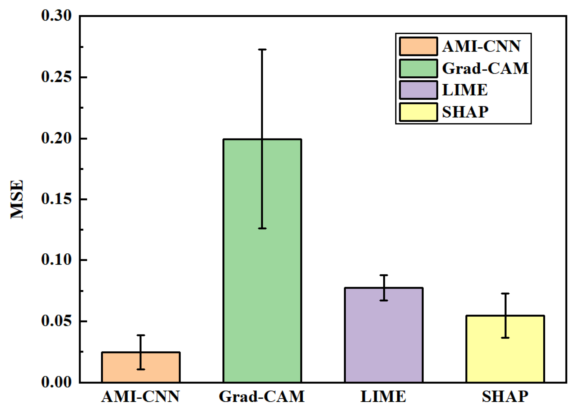
4.3. Quantitative Analysis of Model Interpretability

In the study, we utilize two evaluation metrics, namely, Mean Squared Error (MSE) and the localization-based metric pointing game accuracy (PG-Acc), to quantitatively analyze the constellation phase diagrams.

4.3.1. MSE

Mean Squared Error (MSE) is a commonly used goodness-of-fit metric for evaluating differences between two distributions, defined as

$$MSE={\displaystyle \frac{1}{n}}\sum _{i=1}^n{\left(y_i-\widehat{y_i}\right)}^2$$

(10)

The interpretability of a model can be demonstrated by whether its focus areas align with theoretical expectations. In constellation phase histograms, points with higher frequencies indicate regions where more data points are clustered, suggesting that the model should assign higher weights to these areas. Conversely, points with lower frequencies indicate sparse data regions where the model should assign lower weights. Therefore, MSE can be used to quantify the discrepancy between the model’s focus areas (weight distribution) and the theoretically expected areas (constellation phase histogram frequencies), thereby assessing interpretability. A smaller MSE indicates a better fit of the model.

However, the PSD dataset is not suitable for evaluation using this metric. In PSD theory, the main lobe position is crucial, representing the primary identification features of different modulation formats. Hence, the interpretability of the model largely depends on whether it focuses on the main lobe position. Assigning higher weights to the main lobe position aligns the model with theoretical expectations, demonstrating good interpretability. Conversely, despite potentially larger data values in non-main lobe regions, these areas do not contain key features, and thus, the model should assign lower weights or ignore them. MSE measures the overall difference between two distributions and cannot accurately assess differences between specific regions. Therefore, MSE is not suitable for evaluating the interpretability of the PSD dataset. Ultimately, we only use MSE for evaluation on the constellation phase frequency dataset.

We calculated the MSE for each data sample in the test set and took the mean to represent the MSE between the original data and the weights, aiming to reduce errors. The results are displayed in Figure 8. Overall, the MSE for each modulation format is not high, all below 0.2, within an acceptable range. Specifically, the MSE for AMI-CNN is 0.0246, Grad-CAM is 0.1995, LIME is 0.0775, and SHAP is 0.0547. The lowest MSE is achieved by AMI-CNN, at only 0.0246, indicating superior interpretability compared with other methods.

Figure 9 is a separate plot for each modulation format. Among the three modulation formats, the complexity of the modulation formats follows this sequence: QPSK, 8PSK, and 16QAM, and this trend is also evident in the MSE values, which generally increase accordingly. AMI-CNN achieves the lowest MSE among all modulation formats, with values of 0.1102, 0.2177, and 0.2707 for QPSK, 8PSK, and 16QAM, respectively. LIME and SHAP perform similarly, with LIME slightly outperforming SHAP. Moreover, LIME focuses on local features, making it sensitive to small features. Surprisingly, on the complex modulation format 16QAM, the MSE of LIME decreases by 0.0037 compared with QPSK. In contrast, Grad-CAM exhibits poor performance in MSE, with a significant increase observed, especially on 16QAM. Combining these observations with the images in Figure 7, we notice that Grad-CAM is often insensitive to small features and tends to highlight large block features, leading to poor performance on modulation formats with more detailed features, such as 16QAM.

In summary, AMI-CNN consistently demonstrates the lowest MSE values, both overall and across each modulation format. This indicates that the attention features of AMI-CNN are essentially consistent with the original data, showcasing its optimal interpretability.

4.3.2. PG-Acc

The localization-based metric Point Game [38] is commonly used to measure the precision of interpretable regions, which we refer to as PG-Acc. We call this the Pointing Game, as it asks the CNN model to point at an object of a designated category in the image. Thus, we perform this “pointing” action by extracting the maximum value from the weights and checking if it aligns with the theoretical expectations, to assess whether the model’s interpretable results accurately pinpoint the target regions. The Pointing Game does not require highlighting the entire extent of objects and does not consider the CNN model’s classification accuracy, making it a fair assessment for different types of interpretable techniques. The final accuracy is defined by considering all the data and all the categories within it, as shown in the following formula:

$$PG-Acc\left(all classes\right)={\displaystyle \frac{Hits}{Hits+Misses}}$$

(11)

Figure 10 presents the results for all modulation formats on the constellation phase histogram dataset. Overall, except for the poor performance of LIME, the other three methods achieved relatively high accuracy levels, with PG-Acc for AMI-CNN, Grad-CAM, LIME, and SHAP being 1, 0.9945, 0.4833, and 0.9944, respectively. For the QPSK modulation format, all methods except LIME reached a PG-Acc of 1, whereas LIME’s PG-Acc was only 0.05. As shown in Figure 7, LIME emphasizes phase features primarily distributed in the background region, opposite to the phase clustering points, resulting in a lower PG-Acc. For the 8PSK modulation format, all four methods achieved a PG-Acc of 1. In the most complex 16QAM modulation format, Grad-CAM and SHAP had a PG-Acc of 0.9833, slightly lower than that of AMI-CNN, while LIME’s performance remained poor, with a PG-Acc of only 0.4.

Figure 11 presents the results of the PSD dataset across all modulation formats based on PG-Acc. It can be observed that the AMI-CNN model achieves a PG-Acc of 100% consistently across all modulation formats, demonstrating the best and most stable performance among all models. Grad-CAM performs well with PG-Acc scores of 100% in QPSK and 8PSK but experiences a significant drop to 0% in 16QAM. As shown in Figure 6, Grad-CAM indeed annotates features correctly within the main lobe regions for QPSK and 8PSK but exhibits a substantial change in 16QAM, where annotated areas appear on both sides. This result correlates with the PG-Acc findings, suggesting Grad-CAM’s less precise recognition of smaller targets. In contrast, both LIME and SHAP, two interpretable techniques, appear to perform poorly in this task. Specifically, LIME achieves PG-Acc scores of 0.1333 in QPSK, 0.1 in 8PSK, and 0.2 in 16QAM, while SHAP scores 0.05 in QPSK, 0.2667 in 8PSK, and 0.2 in 16QAM. According to Figure 6, these interpretable techniques also seem not to focus on the main lobe positions in the PSD dataset.

In summary, across both the PSD dataset and the constellation phase histogram dataset, AMI-CNN exhibits the best PG-Acc performance. In terms of this metric, the interpretability demonstrated by AMI-CNN is superior.

5. Conclusions

We propose an Adaptive Mask-Based Interpretable Convolutional Neural Network (AMI-CNN) that enhances model interpretability by selectively emphasizing important features and suppressing less relevant ones through the application of a masking mechanism on multi-channel spatial features during the training process. Additionally, a depthwise convolution is introduced before the fully connected layers to transform local spatial features into global ones, thereby optimizing the decision-making capability of the classifier.

AMI-CNN is compared with other commonly used models on two datasets: PSD and constellation phase histogram. The experimental results demonstrate that AMI-CNN exhibits superior interpretability by effectively explaining its decision-making process through analysis of the model’s attention features.

In the PSD dataset, AMI-CNN primarily focuses on features within the main lobe region, consistent with the theoretical basis of power spectral LIME. In contrast, attention features of LIME and SHAP are more dispersed. Grad-CAM performs well on low-order modulation formats such as QPSK and 8PSK but lacks robustness in identifying key features in more complex 16QAM modulation formats. Due to the unique characteristics of the PSD dataset, we cannot use MSE as an evaluation metric to assess the interpretability of the results. Therefore, we only discuss the performance based on the PG-Acc metric. AMI-CNN achieves 100% PG-Acc across all modulation formats, while Grad-CAM, LIME, and SHAP achieve 66.67%, 14.44%, and 17.22%, respectively. These results further confirm the significant interpretability advantage of the AMI-CNN model.

In the constellation phase histogram dataset, AMI-CNN demonstrates superior interpretability from both qualitative and quantitative perspectives. In qualitative analysis, AMI-CNN accurately identifies features consistent with theoretical expectations and reflects small-scale data variation trends precisely. In quantitative analysis, evaluated using Mean Squared Error (MSE) and the localization-based metric pointing game accuracy (PG-Acc), AMI-CNN achieved the lowest MSE values (0.0114, 0.0197, and 0.0274 for QPSK, 8PSK, and 16QAM, respectively) among all methods. Moreover, AMI-CNN achieved 100% PG-Acc across all modulation formats in the constellation phase dataset, compared with 99%, 98%, and 97% for Grad-CAM, LIME, and SHAP, respectively. In the PSD dataset, AMI-CNN also reached 100% PG-Acc, significantly outperforming other interpretability techniques. These results further highlight the superior interpretability of AMI-CNN.

In conclusion, AMI-CNN demonstrates significant advantages in model interpretability. The alignment of its focused feature regions with optical theory enhances the trustworthiness of its model decisions, which is particularly valuable for non-experts or individuals lacking experience in this field.

6. Discussion

Despite the significant results achieved by the proposed Adaptive Mask-Based Interpretable Convolutional Neural Network (AMI-CNN) in MFI, there are still some limitations that necessitate further research. This paper evaluates the model’s interpretability from two aspects: fitting degree and localization accuracy. However, it neglects stability. Future work could involve using Generative Adversarial Networks (GANs) to synthesize signals and test the algorithm’s robustness against adversarial attacks. This approach may help establish a workflow and metrics for assessing the stability of the methods proposed in this study.

From a practical application perspective, AMI-CNN provides clearer and more precise explanations, aiding engineers in understanding which features critically influence model decisions. This enhanced interpretability can build trust in the model and improve system maintenance and troubleshooting capabilities, which is crucial for modern wireless communication, satellite communication, and other high-reliability and high-performance communication systems.

Theoretically, this study contributes by proposing the AMI-CNN model. By introducing adaptive masks, the model can automatically adjust feature weights during training to better capture and interpret the fine details of signals. This innovation allows for a more nuanced understanding of the “black box” nature of neural networks, potentially leading to improved model performance and interpretability.

References

1. Cheng, Y.; Fu, S.; Tang, M.; Liu, D. Multi-Task Deep Neural Network (MT-DNN) Enabled Optical Performance Monitoring from Directly Detected PDM-QAM Signals. Opt. Express 2019, 27, 19062. [Google Scholar] [CrossRef] [PubMed]
2. Hao, M.; He, W.; Jiang, X.; Liang, S.; Jin, W.; Chen, L.; Tang, J. Modulation Format Identification Based on Multi-Dimensional Amplitude Features for Elastic Optical Networks. Photonics 2024, 11, 390. [Google Scholar] [CrossRef]
3. Jiang, X.; Hao, M.; Yan, L.; Jiang, L.; Xiong, X. Blind and Low-Complexity Modulation Format Identification Based on Signal Envelope Flatness for Autonomous Digital Coherent Receivers. Appl. Opt. 2022, 61, 5991. [Google Scholar] [CrossRef] [PubMed]
4. Wan, Z.; Yu, Z.; Shu, L.; Zhao, Y.; Zhang, H.; Xu, K. Intelligent Optical Performance Monitor Using Multi-Task Learning Based Artificial Neural Network. Opt. Express 2019, 27, 11281. [Google Scholar] [CrossRef] [PubMed]
5. Mohamed, S.E.-D.N.; Al-Makhlasawy, R.M.; Khalaf, A.A.M.; Dessouky, M.I.; Abd El-Samie, F.E. Modulation Format Recognition Based on Constellation Diagrams and the Hough Transform. Appl. Opt. 2021, 60, 9380. [Google Scholar] [CrossRef] [PubMed]
6. Wang, D.; Zhang, M.; Li, Z.; Li, J.; Fu, M.; Cui, Y.; Chen, X. Modulation Format Recognition and OSNR Estimation Using CNN-Based Deep Learning. IEEE Photon. Technol. Lett. 2017, 29, 1667–1670. [Google Scholar] [CrossRef]
7. Xu, J.; Zhao, J.; Li, S.; Xu, T. Optical Performance Monitoring in Transparent Fiber-Optic Networks Using Neural Networks and Asynchronous Amplitude Histograms. Opt. Commun. 2022, 517, 128305. [Google Scholar] [CrossRef]
8. Lv, H.; Zhou, X.; Huo, J.; Yuan, J. Joint OSNR Monitoring and Modulation Format Identification on Signal Amplitude Histograms Using Convolutional Neural Network. Opt. Fiber Technol. 2021, 61, 102455. [Google Scholar] [CrossRef]
9. Wang, F.; Zhou, Y.; Yan, H.; Luo, R. Enhancing the Generalization Ability of Deep Learning Model for Radio Signal Modulation Recognition. Appl. Intell. 2023, 53, 18758–18774. [Google Scholar] [CrossRef]
10. Zhang, Y.; Zhou, P.; Liu, Y.; Wang, J.; Li, C.; Lu, Y. Fast Adaptation of Multi-Task Meta-Learning for Optical Performance Monitoring. Opt. Express 2023, 31, 23183. [Google Scholar] [CrossRef]
11. Fan, X.; Wang, L.; Ren, F.; Xie, Y.; Lu, X.; Zhang, Y.; Zhangsun, T.; Chen, W.; Wang, J. Feature Fusion-Based Multi-Task ConvNet for Simultaneous Optical Performance Monitoring and Bit-Rate/Modulation Format Identification. IEEE Access 2019, 7, 126709–126719. [Google Scholar] [CrossRef]
12. Li, J.; Ma, J.; Liu, J.; Lu, J.; Zeng, X.; Luo, M. Modulation Format Identification and OSNR Monitoring Based on Multi-Feature Fusion Network. Photonics 2023, 10, 373. [Google Scholar] [CrossRef]
13. Hayashi, T.; Cimr, D.; Fujita, H.; Cimler, R. Interpretable Synthetic Signals for Explainable One-Class Time-Series Classification. Eng. Appl. Artif. Intell. 2024, 131, 107716. [Google Scholar] [CrossRef]
14. Adadi, A.; Berrada, M. Peeking Inside the Black-Box: A Survey on Explainable Artificial Intelligence (XAI). IEEE Access 2018, 6, 52138–52160. [Google Scholar] [CrossRef]
15. Zang, Y.; Yu, Z.; Xu, K.; Chen, M.; Yang, S.; Chen, H. Data-Driven Fiber Model Based on the Deep Neural Network with Multi-Head Attention Mechanism. Opt. Express 2022, 30, 46626. [Google Scholar] [CrossRef] [PubMed]
16. Yin, Z.; Chen, B.; Zhen, W.; Wang, C.; Zhang, T. The Performance Analysis of Signal Recognition Using Attention Based CNN Method. IEEE Access 2020, 8, 214915–214922. [Google Scholar] [CrossRef]
17. Zhao, Y.; Shi, C.; Wang, D.; Chen, X.; Wang, L.; Yang, T.; Du, J. Low-Complexity and Nonlinearity-Tolerant Modulation Format Identification Using Random Forest. IEEE Photon. Technol. Lett. 2019, 31, 853–856. [Google Scholar] [CrossRef]
18. Thrane, J.; Wass, J.; Piels, M.; Diniz, J.C.M.; Jones, R.; Zibar, D. Machine Learning Techniques for Optical Performance Monitoring From Directly Detected PDM-QAM Signals. J. Light. Technol. 2017, 35, 868–875. [Google Scholar] [CrossRef]
19. Zhou, H.; Tang, M.; Chen, X.; Feng, Z.; Wu, Q.; Fu, S.; Liu, D. Fractal Dimension Aided Modulation Formats Identification Based on Support Vector Machines. In Proceedings of the 43RD European Conference on Optical Communication (ECOC 2017), Gothenburg, Sweden, 17–21 September 2017; IEEE: New York, NY, USA, 2017. [Google Scholar]
20. Khan, F.N.; Zhou, Y.; Lau, A.P.T.; Lu, C. Modulation Format Identification in Heterogeneous Fiber-Optic Networks Using Artificial Neural Networks. Opt. Express 2012, 20, 12422. [Google Scholar] [CrossRef]
21. Khan, F.N.; Shen, T.S.R.; Zhou, Y.; Lau, A.P.T.; Lu, C. Optical Performance Monitoring Using Artificial Neural Networks Trained With Empirical Moments of Asynchronously Sampled Signal Amplitudes. IEEE Photonics Technol. Lett. 2012, 24, 982–984. [Google Scholar] [CrossRef]
22. Li, S.; Zhou, J.; Huang, Z.; Sun, X. Modulation Format Identification Based on an Improved RBF Neural Network Trained With Asynchronous Amplitude Histogram. IEEE Access 2020, 8, 59524–59532. [Google Scholar] [CrossRef]
23. Jalil, M.A.; Ayad, J.; Abdulkareem, H.J. Modulation Scheme Identification Based on Artificial Neural Network Algorithms for Optical Communication System. J. ICT Res. Appl. 2020, 14, 69–77. [Google Scholar] [CrossRef]
24. Khan, F.N.; Fan, Q.; Lu, C.; Lau, A.P.T. An Optical Communication’s Perspective on Machine Learning and Its Applications. J. Light. Technol. 2019, 37, 493–516. [Google Scholar] [CrossRef]
25. Veerappa, M.; Anneken, M.; Burkart, N.; Huber, M.F. Validation of XAI Explanations for Multivariate Time Series Classification in the Maritime Domain. J. Comput. Sci. 2022, 58, 101539. [Google Scholar] [CrossRef]
26. Liu, H.; Wang, Y.; Fan, W.; Liu, X.; Li, Y.; Jain, S.; Liu, Y.; Jain, A.; Tang, J. Trustworthy AI: A Computational Perspective. ACM Trans. Intell. Syst. Technol. 2023, 14, 1–59. [Google Scholar] [CrossRef]
27. Van Der Velden, B.H.M.; Kuijf, H.J.; Gilhuijs, K.G.A.; Viergever, M.A. Explainable Artificial Intelligence (XAI) in Deep Learning-Based Medical Image Analysis. Med. Image Anal. 2022, 79, 102470. [Google Scholar] [CrossRef] [PubMed]
28. Murdoch, W.J.; Singh, C.; Kumbier, K.; Abbasi-Asl, R.; Yu, B. Definitions, Methods, and Applications in Interpretable Machine Learning. Proc. Natl. Acad. Sci. USA 2019, 116, 22071–22080. [Google Scholar] [CrossRef] [PubMed]
29. Igor, I.; Berk, G.; Mucahit, C.; Gökçe, B.M. Explainable Boosted Linear Regression for Time Series Forecasting. Pattern Recognit. 2021, 120, 108144. [Google Scholar]
30. Sagi, O.; Rokach, L. Explainable Decision Forest: Transforming a Decision Forest into an Interpretable Tree. Inf. Fusion 2020, 61, 124–138. [Google Scholar] [CrossRef]
31. Civit-Masot, J.; Bañuls-Beaterio, A.; Domínguez-Morales, M.; Rivas-Pérez, M.; Muñoz-Saavedra, L.; Corral, J.M.R. Non-Small Cell Lung Cancer Diagnosis Aid with Histopathological Images Using Explainable Deep Learning Techniques. Comput. Methods Programs Biomed. 2022, 226, 107108. [Google Scholar] [CrossRef]
32. Ribeiro, M.T.; Singh, S.; Guestrin, C. “Why Should I Trust You?”: Explaining the Predictions of Any Classifier. In Proceedings of the 22nd ACM SIGKDD International Conference on Knowledge Discovery and Data Mining, San Francisco, CA, USA, 13–17 August 2016. [Google Scholar]
33. Lundberg, S.M.; Lee, S.-I. A Unified Approach to Interpreting Model Predictions. In Proceedings of the Advances in Neural Information Processing Systems 30 (NIPS 2017), Long Beach, CA, USA, 4–9 December 2017; Guyon, I., Luxburg, U.V., Bengio, S., Wallach, H., Fergus, R., Vishwanathan, S., Garnett, R., Eds.; Neural Information Processing Systems (NIPS): La Jolla, CA, USA, 2017; Volume 30. [Google Scholar]
34. Simonyan, K.; Vedaldi, A.; Zisserman, A. Deep Inside Convolutional Networks: Visualising Image Classification Models and Saliency Maps. arXiv 2013, arXiv:1312.6034. [Google Scholar]
35. Zeiler, M.D.; Fergus, R. Visualizing and Understanding Convolutional Networks. In Proceedings of the 13th European Conference, Zurich, Switzerland, 6–12 September 2014; Available online: https://link.springer.com/chapter/10.1007/978-3-319-10590-1_53 (accessed on 15 September 2014).
36. Zhang, Z.; Xie, Y.; Xing, F.; McGough, M.; Yang, L. MDNet: A Semantically and Visually Interpretable Medical Image Diagnosis Network. In Proceedings of the 30th IEEE Conference on Computer Vision and Pattern Recognition (CVPR 2017), Honolulu, HI, USA, 21–26 July 2017; IEEE: New York, NY, USA, 2017; pp. 3549–3557. [Google Scholar]
37. Selvaraju, R.R.; Cogswell, M.; Das, A.; Vedantam, R.; Parikh, D.; Batra, D. Grad-CAM: Visual Explanations from Deep Networks via Gradient-Based Localization. In Proceedings of the 2017 IEEE International Conference on Computer Vision (ICCV), Venice, Italy, 22–29 October 2017; IEEE: Venice, Italy, 2017; pp. 618–626. [Google Scholar]
38. Zhang, J.; Lin, Z.; Brandt, J.; Shen, X.; Sclaroff, S. Top-Down Neural Attention by Excitation Backprop. In Proceedings of the Computer Vision—ECCV 2016, PT IV, Amsterdam, The Netherlands, 11–14 October 2016; Leibe, B., Matas, J., Sebe, N., Welling, M., Eds.; Springer International Publishing Ag: Cham, Switzerland, 2016; Volume 9908, pp. 543–559. [Google Scholar]
Figure 1. Simulation system setup for data acquisition. CW: continuous wave; LO: local oscillation; AD: analog-to-digital converter.
Applsci 14 06302 g001
Figure 2. PSD for three different modulation formats: (a) QPSK, (b) 8PSK, and (c) 16QAM.
Applsci 14 06302 g002
Figure 3. Constellation diagram (top row) and constellation phase histogram (bottom row) corresponding to (a) QPSK, (b) 8PSK, and (c) 16QAM.
Applsci 14 06302 g003
Figure 4. Schematic diagram of the structure for the AMI-CNN model.
Applsci 14 06302 g004
Figure 5. Computation time of AMI-CNN, LeNet, ResNet18, and VGG19 on the PSD dataset and the constellation phase histogram dataset.
Applsci 14 06302 g005
Figure 6. Interpretability results of QPSK on the PSD dataset (the closer the region is to the red color, the greater the weight, representing the more attention the model pays to the feature).
Applsci 14 06302 g006
Figure 7. Interpretability results of QPSK on the constellation phase histogram dataset (the closer the region is to the white color, the greater the weight, representing the more attention the model pays to the feature).
Applsci 14 06302 g007
Figure 8. MSE of interpretability methods on the constellation phase histogram dataset: AMI-CNN, Grad-CAM, LIME, and SHAP.
Applsci 14 06302 g008
Figure 9. MSE of different interpretability methods for three modulation formats on the constellation phase histogram dataset: QPSK, 8PSK, and 16QAM.
Applsci 14 06302 g009
Figure 10. Comparison of PG-Acc for different modulation formats on the constellation phase histogram dataset.
Applsci 14 06302 g010
Figure 11. Comparison of PG-Acc for different modulation formats on the PSD dataset.
Applsci 14 06302 g011