Optimizing Automated Detection of Cross-Recessed Screws in Laptops Using a Neural Network

Abstract

This paper investigates varying the operating conditions of a neural network in a robotic system using a low-cost webcam to achieve optimal settings in order to detect crossed-recess screws on laptops, a necessary step in the realization of automated disassembly systems. A study was performed that varied the lighting conditions, velocity, and number of passes the robot made over the laptop, as well as the network size of a YOLO-v5 neural network. The analysis reveals that specific combinations of operating parameters and neural network configurations can significantly improve detection accuracy. Specifically, the best results for the majority of laptops were obtained when the system ran at medium velocity (10 and 15 mm/s), with a light, and the neural network was run with an extra large network. Additionally, the results show that screw characteristics like the screw hole depth, the presence of a taper in the screw hole, screw hole location, and the color difference between the laptop cover and the screw color impact the system’s overall detection rate, with the most important factor being the depth of the screw.

1. Introduction

As consumer demand for electronic products continues to grow, and the lifespan of these items shortens, the issue of how to handle discarded electronic waste (e-waste) remains a pressing global concern [1]. In 2019, it was estimated that 53.6 million metric tons (Mt) of e-waste was generated globally; however, only 17.4% (9.3 Mt) was actually recycled through official channels. By 2030, it is predicted that the amount of e-waste generated will be close to 74 Mt [2]. The European Commission has classified e-waste into six distinct categories: temperature and exchange equipment, screens and monitors, lamps, large equipment, small equipment, and small information technology (IT) and telecommunication equipment [3], which are shown in

Table 1. E-waste categories, as defined by the European Commission, examples, and e-waste generated (overall and percentage increase) [2].

E-Waste Category	Product Examples	Total E-Waste Generated in 2019 (Mt)	Percentage of Total E-Waste (%)	Percentage Increase from 2014 to 2019 (%)
Temperature and exchange equipment	Refrigerators, freezers, air conditioners, and heat pumps	10.8	20.1	+7
Screens and monitors	Televisions, monitors, laptops, and tablets	6.7	12.5	−1
Lamps	Fluorescent lamps, high intensity discharge lamps, and LED lamps	0.9	1.7	+4
Large equipment	Washing machines, dryers, electric stoves, and copying equipment	13.1	24.4	+5
Small equipment	Vacuums, microwaves, toasters, calculators, electronic toys, and electronic tools	17.4	32.5	+4
Small IT and telecommunications equipment	Mobile phones, GPS devices, routers, personal computers, printers, and telephones	4.7	8.8	+2

.

E-waste has historically been exported from developed countries to less regulated regions in the developing world, where environmental and disposal regulations are less strict [4]. Despite legislation aimed at addressing this issue, such as the Basel Convention [5], the amendment to the European Union Waste Shipment Regulations [6], and a number of regulations from China, such as the Prohibition of Foreign Garbage Imports and others [7], the unlawful practice of shipping e-waste to less regulated areas persists [8]. The majority of e-waste is then subjected to disposal methods that are hazardous for both the individuals responsible for recycling and the environment. Various studies have examined the impact e-waste recycling has on both workers and the environment in these areas [9,10,11]. These disposal practices include incineration, burial, or the dumping of e-waste into bodies of water [12]. E-waste comprises valuable materials and components, which makes the disassembly and recovery of specific costly components economically attractive [13].

1.1. Related Work in Robotic Disassembly

In response to the above issues, robotic disassembly offers a promising solution to the challenges posed by e-waste recycling. Disassembly robots would be able to handle hazardous conditions and toxic substances found in e-waste without endangering human health. By recovering valuable resources like rare metals efficiently and reducing the environmental impact, robotic disassembly could also make e-waste recycling more economically viable by reducing labor costs [14].

Currently, few commercial systems exist that can disassemble complete electronic products. Fuji Film Co., Ltd. (Tokyo Japan) created a system that could completely sort and disassemble single-use cameras without any manual intervention [15]. In 2016, Apple announced the Liam system, a series of robotic arms and work cells that could disassemble iPhone 6 models. This was improved in 2018 with the Daisy system, which could differentiate and disassemble nine different iPhone models [16].

Vonbunyong et al. [17,18,19] presented a system that could disassemble liquid crystal display (LCD) TVs. This system used a cognitive agent to decide on the next step in the disassembly process. The system was expanded by Foo et al. [20,21], who designed a learning framework that used a database of previous disassembly experiences to create rules and relationships between different components to aid disassembly runs. DiFilippo and Jouaneh [22] designed a robotic disassembly system that utilized multiple cameras and a sensor-equipped screwdriver tool to find and remove screws from the back of laptops and then integrated the cognitive architecture SOAR [23] to remember the location of screws on various laptop models to improve disassembly times.

Previous research on automated disassembly has primarily concentrated on developing tools and strategies for unscrewing operations. Li et al. [24] created an unfastening tool that used torque and position sensing to monitor when the screw was removed, and a spiral control strategy to help the tool mate with the screw and overcome positioning errors. Chen et al. [25] proposed a method in which images of a screw were used to facilitate the orientation of the screw–tool engagement and torque monitoring was used during screw removal process. Klas et al. [26] designed the KIT gripper, which is a multi-functional, five-degree-of-freedom robot arm and gripper that can rotate and close. Moreover, there are several companies that manufacture automated screwdriver end effectors for assembly, which could be used for screw removal tasks. These end effectors include the OnRobot Screwdriver by On Robot [27], capable of handling screws with sizes ranging from M1.6 to M6 and lengths of up to 50 mm. Additionally, the MicroTorque QMC series screwdrivers from Atlas Copco [28] are designed for low-torque applications and are known for their lightweight construction.

Other tools that have been designed include prying tools to separate housing components for LCD displays [29] and part of cellphone [30], and a tool that could depress and remove snap-fits by Schumacher and Jouaneh [31,32].

1.2. Related Work in Vision Detection

In disassembly processes, it is crucial to identify fasteners, which are connectors used to join and hold various parts together. For direct recycling methods, it is critical to identify the locations of these fasteners so the parts they are holding together can be released and reused. In the robotic system designed by DiFilippo and Jouaneh [22], two webcams were used; one mounted above the workspace to locate screws using a Hough circle transform and the other mounted on the robot to verify screws by varying computer vision parameters. Gil et al. [33] used an adaptive thresholding technique to expose contour information. An approach by Büker et al. [34] described a technique that combined contour identification and principal component analysis (PCA) with eigentemplates to identify car wheels and their bolts. Bdiwi et al. [35] proposed a method that also used a PCA approach with a Harris detector to detect the edges and corners of the screw.

Object detection, the act of finding specific objects in images, is playing an ever-increasing role in various industries and applications [36]. Ever since Krizhevsky et al. [37] introduced AlexNet in 2012, convolutional neural networks (CNNs) have become the predominant method to perform object detection, and they have spawned advanced architectures such as Faster Regions with CNN (R-CNN) [38], You Only Look Once (YOLO) [39], and the Single Shot MultiBox Detector (SSD) [40], amongst others [41].

Recently, deep learning methods in object recognition have started to be employed to locate and identify fasteners. Yildiz and Wörgötter [42,43] presented an approach using Hough transforms and two deep CNNs for the detection of screws of variable shapes and sizes on computer hard drives. They designed and deployed an integrated model using InceptionV3 and Xception that generated an average precision of 80.23%. Brogan et al. [44] explored screw detection on general electronics using the tiny-YOLOv2 model, specifically how to optimize the hyperparameters of mini-batch size and resolution for best results. They determined that, for the GPU they were using, a mini-batch size of 16 and input resolution of 1664 × 1664 px produced a mean average precision (mAP) greater than 90% with all their test sets.

Foo et al. [45] investigated using pre-processing adjustments (brightness and contrast) on screws for use with a model pre-trained with the Common Objects in Context (COCO) dataset using Faster R-CNN with the Inception v2 framework. The results were then compared against common screw locations on products to find any undetected screws. Li et al. [46] used a Faster R-CNN network to find screws from complex mobile phone boards. They also used a rotation edge similarity algorithm to improve the location accuracy of the results and reported a classification percentage of 99.64% and a localization deviation of 0.094 mm. Mangold et al. [47] used 550 training images to train two different YOLOv5 networks to classify six different classes of screw heads and achieved a similar mAP of 0.5:0.95 over 0.82 for both network models. They concluded that a YOLOv5-S network worked better than a YOLOv5-m model because it had significant runtime advantages while maintaining similar accuracy. Zhang et al. [48] used a YOLOv4 network to detect screws and an EfficientNetv2 to help eliminate detection errors in order to detect three types of screws. Peralta et al. [49] presented an approach to detect a hex-head fastener and its rotational orientation using a segmentation neural network. A two-stage detection framework was proposed by Liu et al. [50] to detect screws under non-uniform lighting conditions. In their framework, the first stage is used to extract used and structurally damaged screws, and the second stage is used to filter out false areas based on reflections. Li et al. [51] proposed a method called “Active Screw Detection” in which a camera attached to a robotic arm is moved around to align with the normal vector of the screw pointing out of a plane to determine the best image of a screw. The images are fed to a YOLOX-s network, and this method was able to obtain a mAP of 95.92%.

The objective of this study was to experiment with various operational parameters within a robotic system specifically designed for screw removal. The goal was to identify the optimal settings for screw detection. The parameters under investigation encompass mechanical collection aspects, such as the system’s velocity and the number of passes it makes over the laptop, as well as the system’s lighting conditions. Additionally, variations in the network size parameters of the YOLO-v5 neural network were explored. While there have been several works on screw detection [42,43,44,45,46,47,48,49], we found no reported work that analyzes how different screw characteristics impact the detection of these screws. Thus, a unique contribution of this work, and a motivation for this study, is the analysis of how different screw characteristics, such as their location, their color contrast with the laptop, their depth, or the presence of a taper in the screw hole, impact the overall detection rate of the system.

The remainder of this paper is organized as follows. The next section discusses the robotic setup, the software methods used to train the neural networks, and the experimental approaches used to perform the trials. This is followed by Section 3, which presents the results obtained, and Section 4, which is a discussion of the results. Finally, Section 5 provides concluding remarks.

2. Materials and Methods

2.1. Software Methodology

A dataset of 900 cross-recessed screws (CRSs) on electronic equipment was obtained from Brogan et al. [44]. https://github.com/Dan-Brogan/Cross-Recessed-Screw_Deep-Learning-Datasets (accessed on 11 May 2023). These images had a size of 4048 × 3036 pixels (px) and were imported into Roboflow for annotation by drawing bounding boxes around the CRS in each image. The dataset was divided into three sets for training, validation, and testing. The training set consisted of 630 images, the validation set included 180 images, and the testing set contained 90 images. The dataset images were preprocessed to a resolution of 640 × 480 px, which was compatible with the camera mounted on the robot. Two YOLOv5 models were trained using an NVIDIA GeForce RTX GPU 3070Ti (Windows 10, 32 GB RAM). These models included the YOLOv5-Small (YOLOv5-S) and YOLOv5-Extra large (YOLOv5-XL) variants, each with square image sizes of 640 px. Neural networks can be described with parameters, as described by [52], and full details of the YOLOv5 networks can be found in [53]. The models were trained for a maximum of 1000 epochs with early stopping enabled, allowing training to stop if no improvement was observed in the last 100 epochs. Additionally, the models were trained with the maximum batch size that the GPU could accommodate. For the YOLOv5-S models, the batch size was set to 16, and for the YOLOv5-XL model, the batch size was set to 8. Additionally, to verify that the models were adequately trained, the mAP of the test set was calculated for each of the models, and it was 0.976 for YOLOv5-S and 0.985 for YOLOv5-XL.

2.2. Experimental Methodology

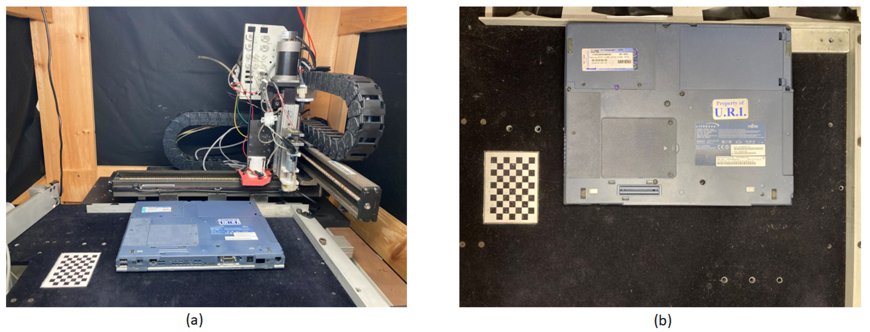
The robotic platform used was a customized ENCore 2s System (MRSI, North Billerica, MA, USA) controlled with a Galil DMC-2413 controller. This controller was integrated with Python version 3.7.9 and gclib version 1.37.6. The system was connected to a computer (Windows 10, 16 GB RAM, NVIDIA GeForce RTX 3070). The robotic platform was enclosed within a wooden frame equipped with detachable black sheets designed to exclude external light sources. Within this frame, a platform covered in black felt serves as the designated placement area for the laptops. A low-cost webcam (Microsoft Lifecam 3000-HD) was positioned on the head of the Cartesian robot, which is capable of lateral and vertical movement across the laptop cover to capture images for experimental trials. The camera is surrounded by a skirt that houses 4 LEDs that can illuminate the surface underneath the camera. The robot’s origin and the laptop’s origin were offset with an 85 mm spacer in the X direction to ensure complete coverage via the webcam. Inside the wooden frame, two under-cabinet light strips were positioned above the platform, providing internal illumination. The operational area, where the laptop was positioned for trial testing, is depicted in Figure 1.

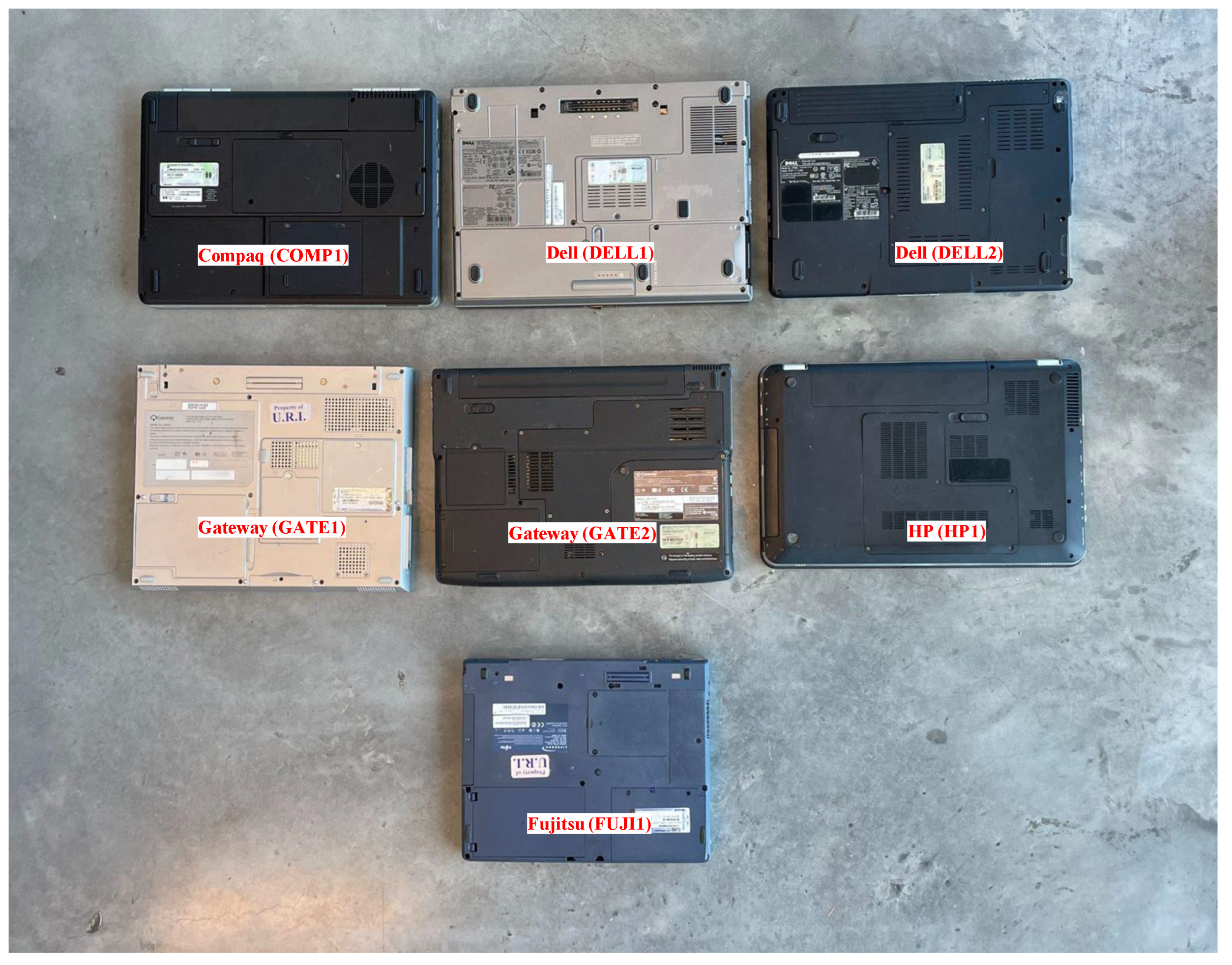
Testing involved seven different used laptops, which were labeled according to their respective manufacturers and displayed in Figure 2. A test consisted of the robotic system making a certain number of passes at a set velocity over the laptop while the webcam continuously captured images. In addition to recording the image, the X and Y positions of the robot were logged at every recorded frame. For these trials, a laptop was always positioned so that its hinge was facing away from the robot. 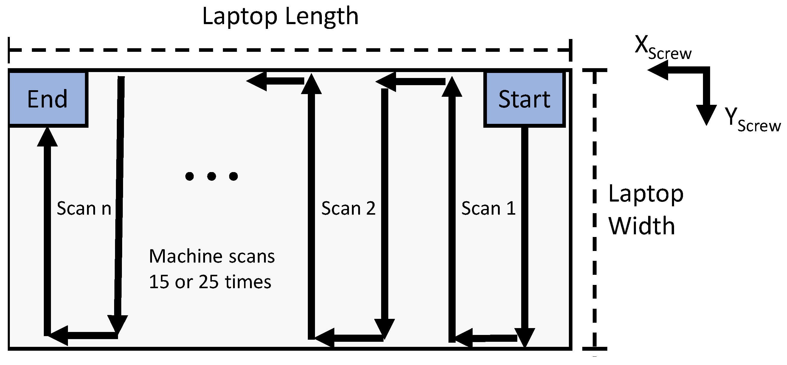Figure 3 shows the movement pattern during the test. The camera started from the top right (the laptop’s origin) and moved in the positive Y direction toward the hinge of the laptop. One scanning pass was defined as the robot moving toward the hinge, traveling a predefined distance parallel to the hinge in the positive X direction, and then moving away from the hinge. This pattern was repeated over the length of the entire laptop. The location and characteristics of the screws in each of the seven laptops were measured with a caliper that had a ${12}^{″}$ range, a ${0.001}^{″}$ graduation, and a ${0.1}^{″}$ displacement per revolution (MSC Industrial Supply).

2.3. Screw Detection Accuracy Methodology

The testing matrix is presented in

Table 2. Testing parameters and their corresponding testing abbreviations used throughout the study.

Parameters	Categories	Abbreviations
Velocity	4 choices ( 5, 10, 15, 20 mm/s)	V5, V10, V15, V20
Number of ccans	2 choices (15, 25 scans)	S15, S25
Lighting	2 choices (with light, no light)	wl, nl
Neural network size	2 choices (YOLOv5-small, YOLOv5-Extra large)	S, XL

. All the laptops were run at four different velocities (5, 10, 15, or 20 mm/s), with 15 and 25 passes over the laptop, and with and without an LED light. With these parameters, each laptop was run through the machine 16 times (112 total trials), and each of these 112 trials was processed through the two YOLO neural networks of different sizes (S or XL) using a confidence threshold of 0.5 for positive detections resulting in a total of 224 tests (32 per laptop). Due to the number of trials, a naming system was devised, which will be referred to in the results. An example of the conceived naming system is V10_S15_XL_wl, in which each operating condition is labeled and separated with an underscore (velocity—10 mm/s, scans—15, neural network size—xl, and lighting condition—with light).

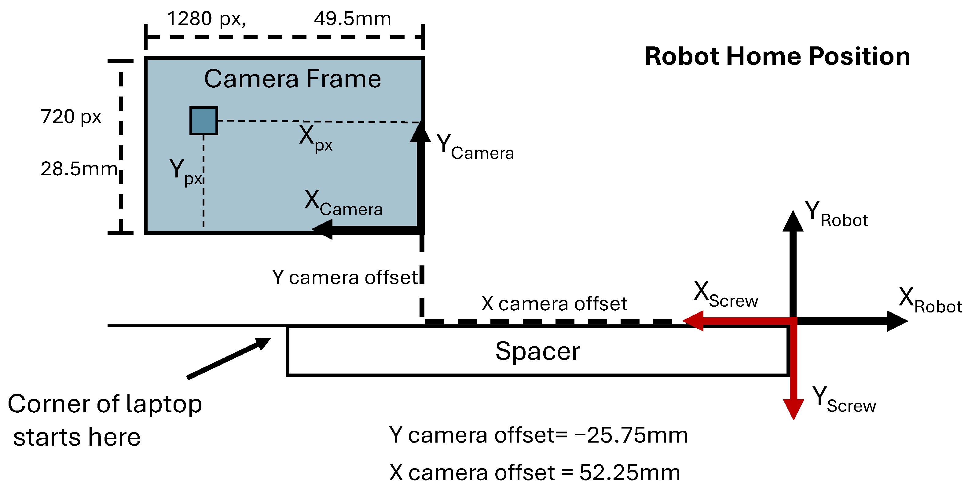
To address the possibility of detecting the same screw multiple times in consecutive frames as the robot moves over the laptop and continuously captures images, the software employs a method to determine the screw’s position relative to a screw coordinate frame established when the robot is initially homed. This coordinate system’s configuration at the home position is illustrated in Figure 4. The location of a screw within the screw coordinate frame can be calculated using Equations (1) and (2). Here, $x_{px}$ and $y_{px}$ represent the pixel coordinates of the screw’s location, while $X_{robot}$ and $Y_{robot}$ denote the robot’s current position. It is worth noting that the camera utilized in this setup has a resolution of 1280 × 720 px, which corresponds to an image with a field of view measuring 49.5 mm × 28.5 mm. Additionally, the camera’s origin was offset from the screw’s origin by 52.25 mm in the X_Screw direction and −25.75 mm in the Y_Screw direction.

$$X_{screw}={\displaystyle \frac{x_{px}}{1280}}\times 49.5+(-X_{robot}+52.25)$$

(1)

$$Y_{screw}=-{\displaystyle \frac{y_{px}}{720}}\times 28.5+(-Y_{robot}-25.75)$$

(2)

2.4. Screw Characteristic Analysis Methodology

To gain deeper insights into the data regarding the detection and misidentification of individual screws, it is essential to identify potential trends among screws with varying detection rates. In pursuit of this goal, a comprehensive analysis was conducted using all 115 screws sourced from the seven different laptops. Each screw was examined to gather data on specific attributes. These attributes were categorized into four primary categories:

• Depth: Screws were classified as either deep or surface screws.
• Location: The location of each screw was categorized as either belonging to the corner, exterior, or interior of the laptops.
• Color difference: The extent of color contrast between the laptop case and the screw head was assessed and grouped into categories of large, medium, or small color differences.
• Taper presence: An evaluation was made to determine whether each screw hole exhibited a taper or not.

In the depth category, screws were categorized based on whether they were recessed more than 0.10 inches (2.5 mm) from the laptop cover’s surface. Additionally, screws were designated as “exterior screws” if they were positioned within 0.785 in (approx 20 mm) from the laptop’s side. Within the exterior screws category, a specific subset was identified as “corner screws”, referring to screws situated between two sides of the laptop near the edges. The presence of a taper on a screw was noted when the laptop’s surface exhibited an uneven depth around it. The screws were also subject to an evaluation of their color, which included the options of silver, black, or light black. Additionally, the laptops themselves were examined for their color, which could fall into categories blue, black, or silver. These combinations were then organized into three distinct color difference categories:

• Large color difference: This category included instances in which black screws were paired with a silver laptop or silver screws were matched with a black laptop.
• Medium color difference: This category encompassed situations where light black screws were paired with a black laptop or light black screws were matched with a blue laptop.
• No color difference: This category involved cases in which black screws were matched with a black laptop or silver screws were paired with a silver laptop.

3. Results

3.1. System Detection Accuracy

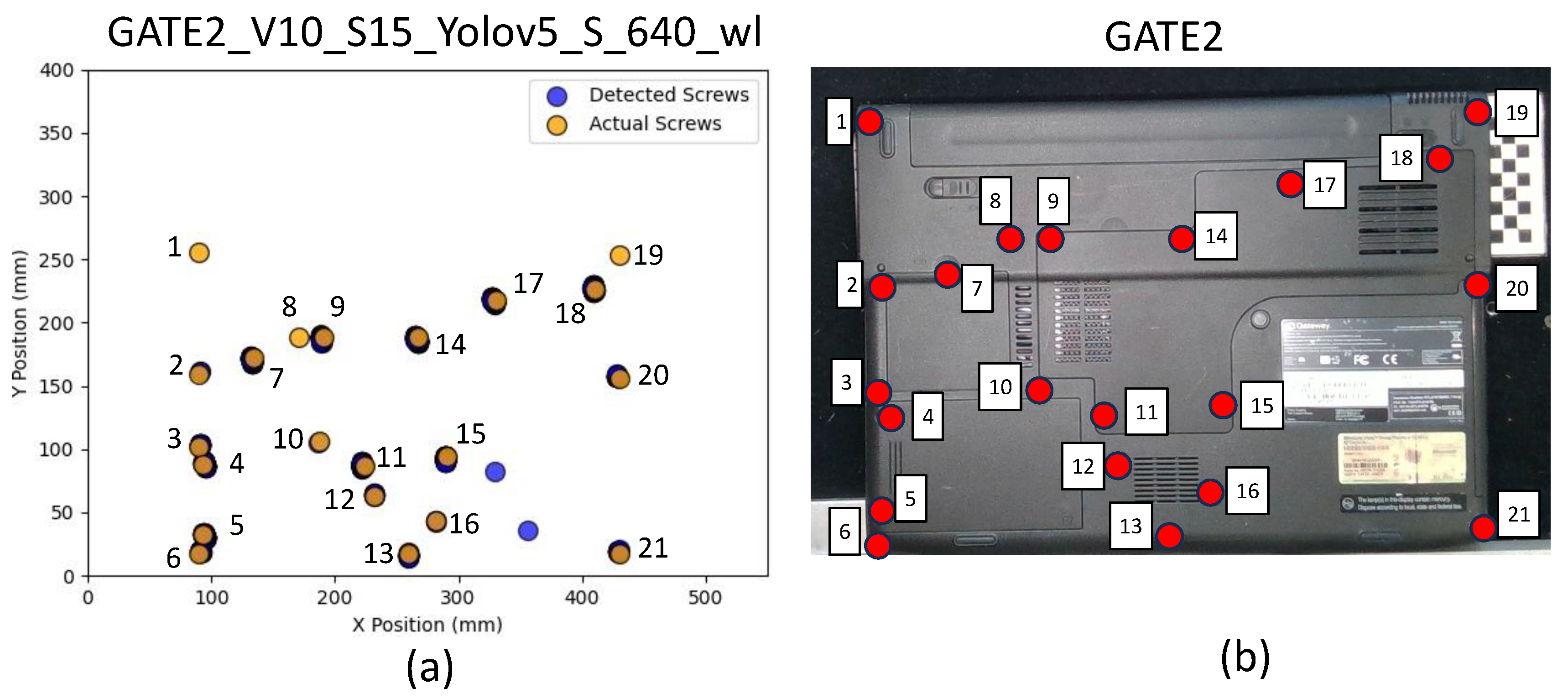
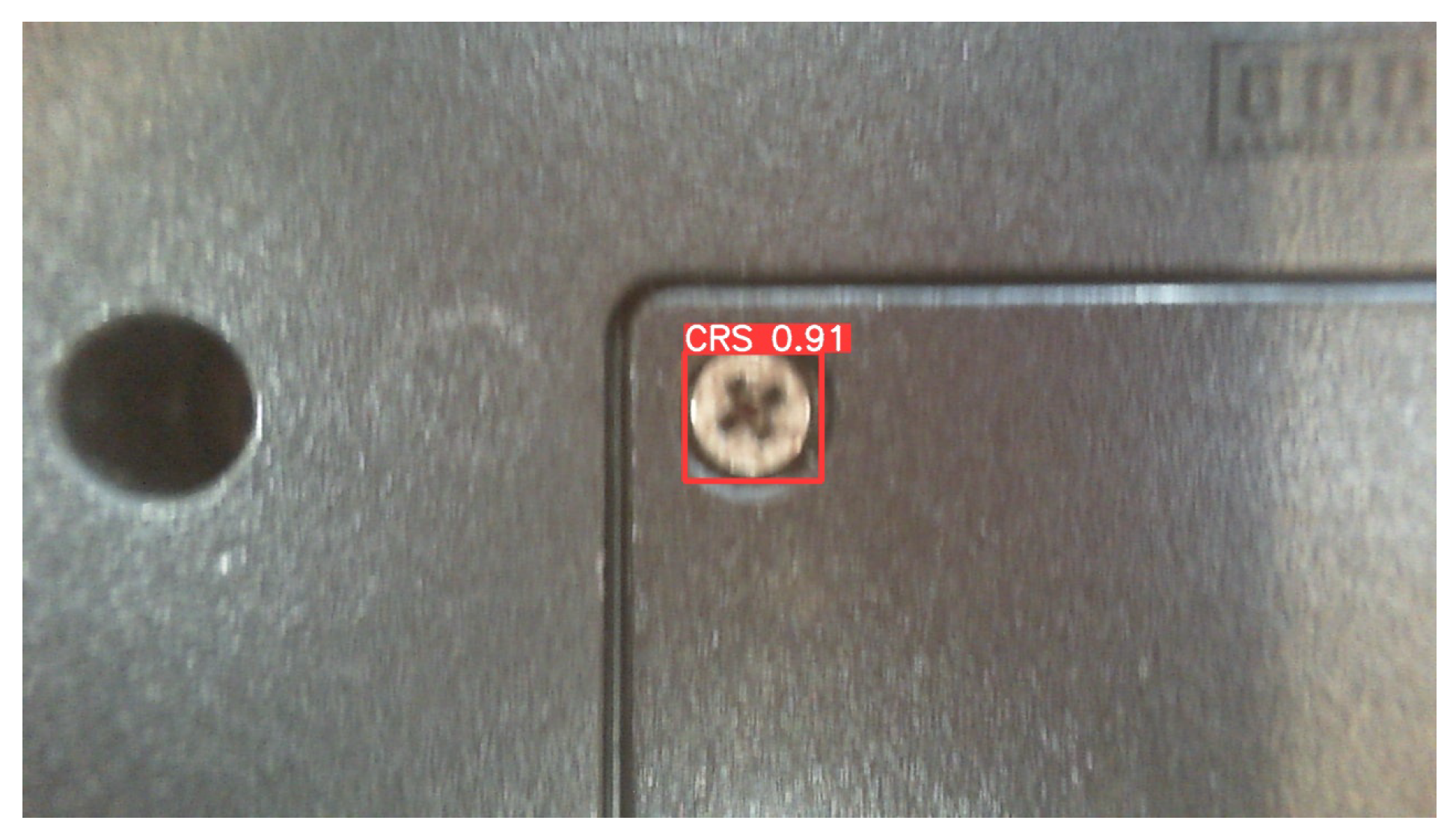
This section presents the findings of the study focused on determining the optimal operating conditions for a robotic system and neural network. To illustrate the results, we present a coordinate map, as shown in Figure 5, which depicts the locations of actual screws on a laptop alongside the locations detected via the neural network, using GATE2 as an example (all laptops and their screw numbers can be found in S1-Coordinate Maps.pdf in the Github repository). In this analysis, a successful detection will typically occur when a blue circle (detected screw) intersects with an orange circle (actual screw), indicating that the neural network correctly identified the screw’s location. The output images of the neural net, shown in Figure 6, can be checked to ensure that false detections are not located near a detected screw. Due to the movement of the robotic system between images, the positions of the screws may exhibit slight variations, leading to asymmetrical appearances in the blue circle areas at times. For the GATE2 laptop data, there were a total of 21 screws on the laptop, and in the example trial shown, the neural network successfully identified 18 of them. However, three detections were missing (Screw 1, Screw 8, and Screw 19), and there were two false detections in which features other than screws (in this case specifically, stickers) were mistakenly identified and marked in the graph with isolated blue circles. A further discussion of false detections is provided in Section 3.1, Screw Characteristic Analysis.

The information from the coordinate maps could be used to create

Table 3. True and false detection for GATE2 laptop. True detections are when the system correctly determines a screw, and false detections are when the system incorrectly classifies a feature as a screw.

	Number of True Detections				Number of False Detections				Vision Accuracy Percentage
Trial Name	V5	V10	V15	V20	V5	V10	V15	V20	V5	V10	V15	V20
S15_S_nl	19	18	15	9	3	1	2	0	76.2	81.0	61.9	42.9
S15_S_wl	21	18	17	8	8	2	0	1	61.9	76.2	81.0	33.3
S15_XL_nl	19	18	15	10	0	0	0	0	90.5	85.7	71.4	47.6
S15_XL_wl	21	19	17	12	2	0	0	0	90.5	90.5	81.0	57.1
S25_S_nl	19	20	14	12	4	0	0	1	71.4	95.2	66.7	52.4
S25_S_wl	20	20	18	12	6	1	2	2	66.7	90.5	76.2	47.6
S25_XL_nl	18	18	15	10	0	0	0	1	85.7	85.7	71.4	42.9
S25_XL_wl	20	18	16	12	3	0	0	0	81.0	85.7	76.2	57.1

, which provides a comprehensive view of true detections, false detections, and the vision accuracy parameter, focusing on the GATE2 laptop and broken down according to trial velocity (tables for all laptops can be found in S2-Vision Accuracy.xlsx in the Github repository). For the GATE2 laptop, the “Number of True Detections” column shows the number of correctly identified screws out of a total of 21 on the laptop. Meanwhile, the “Number of False Detections” column indicates how many times the system incorrectly identified screws (or clusters of false detections) in non-screw locations. The values in the “Vision Accuracy Percentage” column were determined using the formula shown in Equation (3). This formula combines two critical aspects of a successful laptop analysis: achieving a high percentage of true detections and minimizing false detections. The resulting percentage serves as a corrected accuracy measure, accounting for the presence of false detections. It should be noted that this formula can allow the percentage to be negative, which means the trial had more false detections than true detections.

$$\mathrm{Vision} \mathrm{Accuracy} = {\displaystyle \frac{\mathrm{Number} \mathrm{of} \mathrm{True} \mathrm{Detections} - \mathrm{Number} \mathrm{of} \mathrm{False} \mathrm{Detections}}{\mathrm{Number} \mathrm{of} \mathrm{Total} \mathrm{Screws} \mathrm{on} \mathrm{Laptop}}}\times 100$$

(3)

Table 4. Average vision accuracy for all laptops broken down by velocity.

	Vision Accuracy by Velocity
Trial Name	V5	V10	V15	V20	Average of All Trial Velocities
S15_S_nl	48.7	58.1	41.2	29.7	44.4
S15_S_wl	37.8	62.7	54.3	38.6	48.3
S15_XL_nl	64.7	69.9	61.9	42.1	59.7
S15_XL_wl	65.1	72.7	68.7	58.4	66.2
S25_S_nl	45.8	58.1	40.0	28.1	43.0
S25_S_wl	24.9	52.0	50.9	43.9	42.9
S25_XL_nl	60.8	68.8	61.7	47.6	59.7
S25_XL_wl	55.4	66.1	73.4	54.6	62.7

presents the vision accuracy average for all the laptop models, broken down according to the velocity of the robot. The “Average of all the Trial Velocities” column represents the mean vision accuracy across the “V5”, “V10”, “V15”, and “V20” columns, and it reveals several key insights. Firstly, it highlights that the YOLOv5-XL model outperformed the YOLOv5-S model. Furthermore, the data suggest that, on average, the results were more favorable when the LED light was employed as opposed to when it was turned off. They also show that the number of passes the robot made over the laptop tended not to cause any change in vision accuracy. When examining columns V5 through V20, a notable trend emerges: medium velocities, specifically velocities of 10 and 15 mm/s, tended to deliver better performance on average within a trial group compared to slower or faster velocities, i.e., velocities of 5 and 20 mm/s.

According to these observations, the four best trial groups based on their vision accuracy percentages among various combinations were as follows:

• V15_S25_XL_wl—73.4%
• V10_S15_XL_wl—72.7%
• V10_S15_XL_nl—69.9%
• V10_S25_XL_nl—68.8%

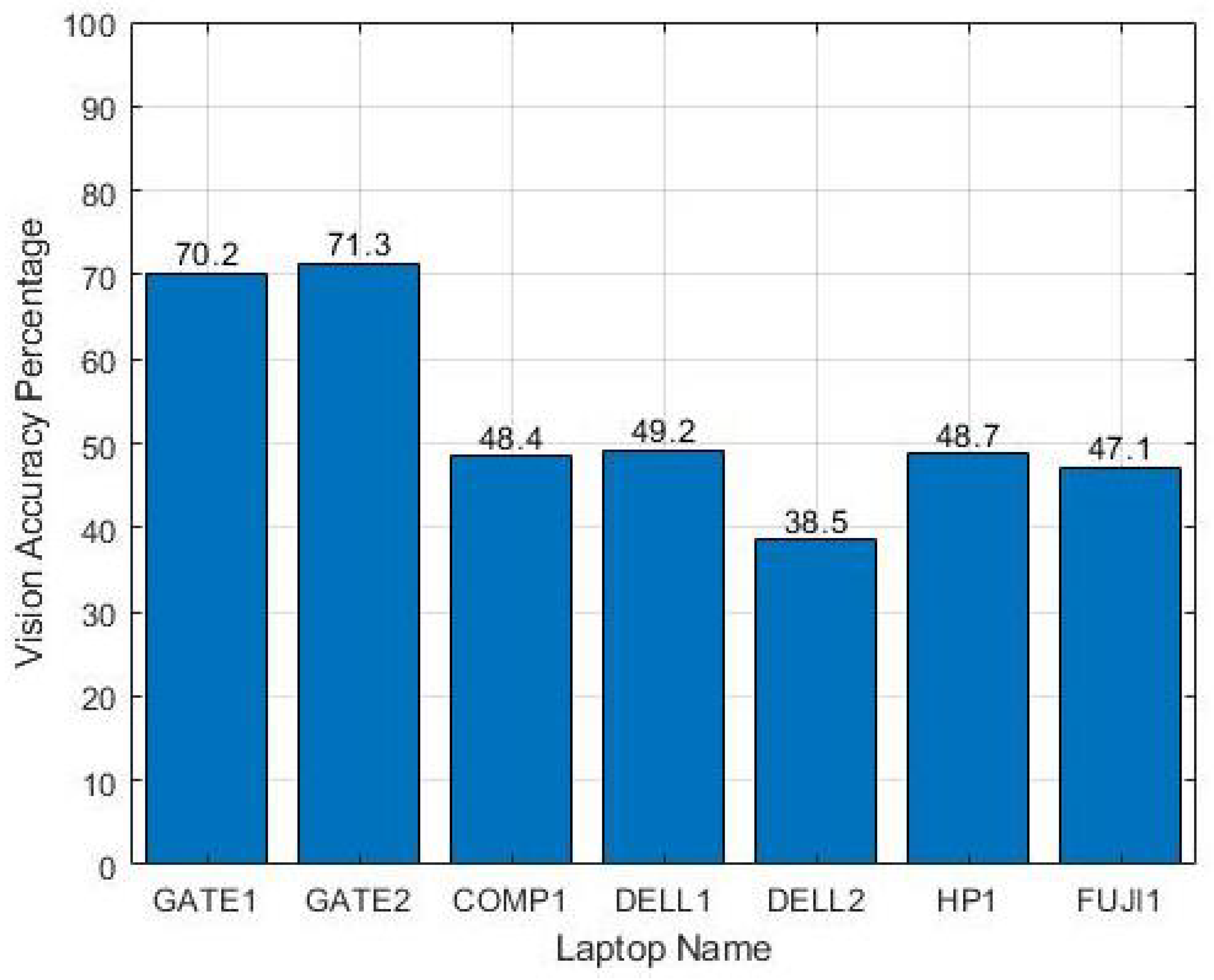
After the trial groups with the highest detection rates were identified, the next step involved examining the disparities in detection rates among different laptops. In Figure 7, the overall vision accuracy percentage across all trials is calculated and presented for each laptop. GATE1 and GATE2 emerged as the best-performing laptops, achieving an overall vision accuracy percentage of 70.2% and 71.3%, respectively. On the other hand, the lowest overall detection rate, 38.5%, was observed in the data for DELL2. A closer look at the differences between the higher- and lower-performing laptops revealed that GATE1 featured a silver case and silver screws, GATE2 had a black case and silver screws, while DELL2 had black cases with black screws. Additionally, it was noted that GATE1 had a mix of surface screws and deep screws, whereas COMP1 had no surface screws. DELL2 also had deeper screws located near other features that were being recognized as false detections. Both of these factors were identified as potential contributors to the differences in detection rates, and they required further investigation. It should be noted that these overall vision accuracy percentages are an average of particular laptop trials, and an individual trial could have yielded higher percentages. The vision accuracy percentage for all the individual trials can be found in S2 - Vision Accuracy.xlsx.

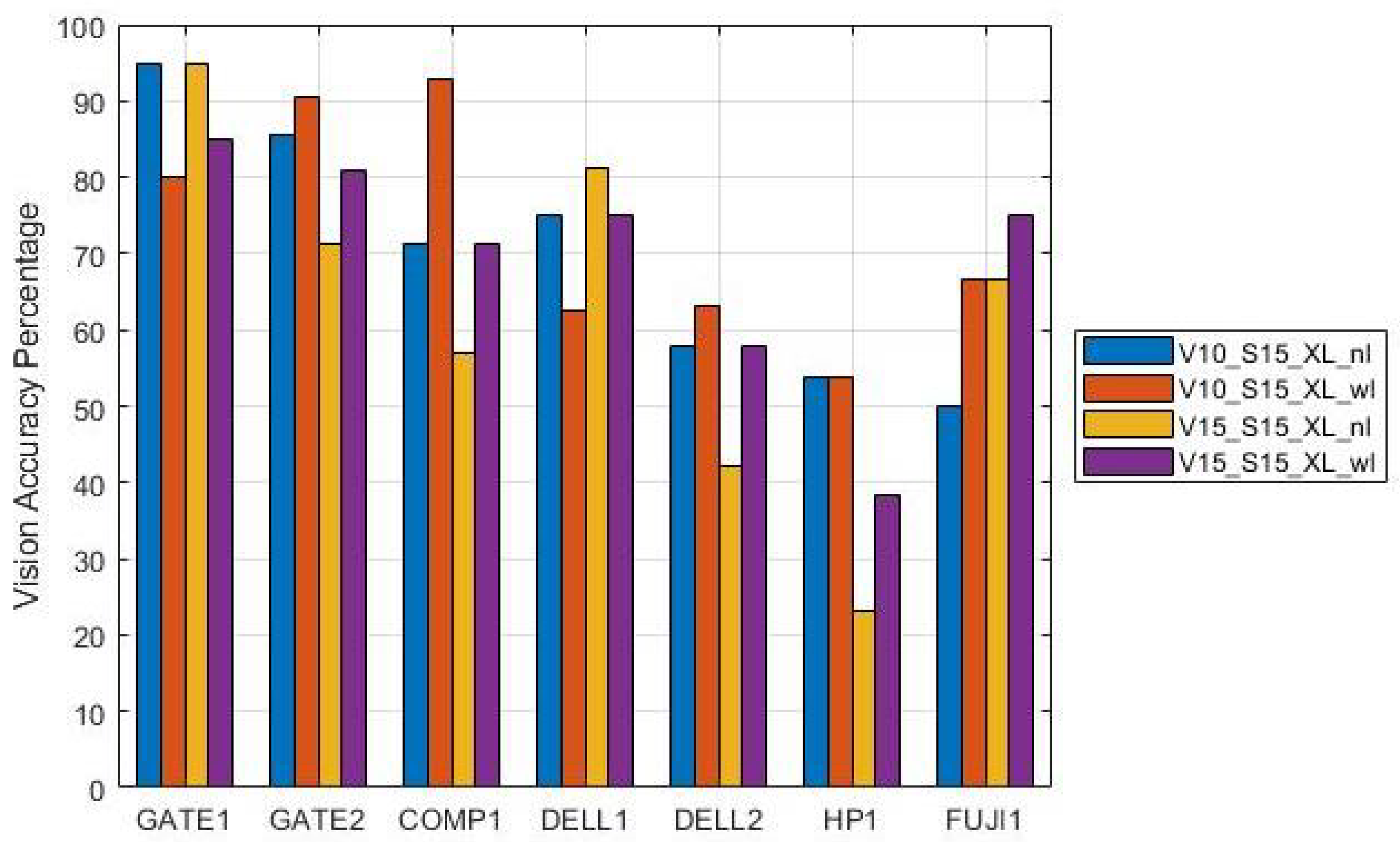
To further investigate the effect that light has on detection accuracy, a few high-performing trials were chosen at two different velocities (V10 and V15), and the lighting parameter was varied (nl and wl). Figure 8 displays the vision accuracy percentage broken down by laptop. For example, two trials for the Gate1 laptop (V10_S15_XL_nl and V15_S15_XL_nl) achieved vision accuracy of 95%. The results highlight that DELL2 and HP1 tended to be the laptops with the lowest accuracy amongst this subset of trials. Both DELL2 and HP1 demonstrated improved detection accuracy when additional lighting was introduced. Interestingly, two laptops experienced decreased accuracy when exposed to light, while all the other laptops either performed better or maintained their vision accuracy. Specifically, GATE1 and DELL1 were the only two laptops that showed a decline in their vision accuracy percentage. It should be noted that both of these laptops are a lighter color, and when subjected to additional light, they exhibited more false positives than increases in true positives.

3.2. Screw Characteristic Analysis

This section displays the results of the analysis performed on the screw characteristics of all 115 screws found on the laptops. Here, the dataset was divided into 16 trials through which the results and statistics of individual screws could be tallied. The trials included varying LED lighting conditions (on and off), as well as different velocities (10 and 15 mm/s) and passes (15 and 25), and employing different sizes of the YOLOv5 neural networks (S and XL). For each laptop and in each of these trial runs, data were collected for both true detections and false detections, with location and classification information recorded for the false detections. These detection results were then aggregated to calculate the overall percentage of detection for each screw, which could range from 0% to 100%. Additionally, all data related to false detections were compiled and subjected to further analysis.

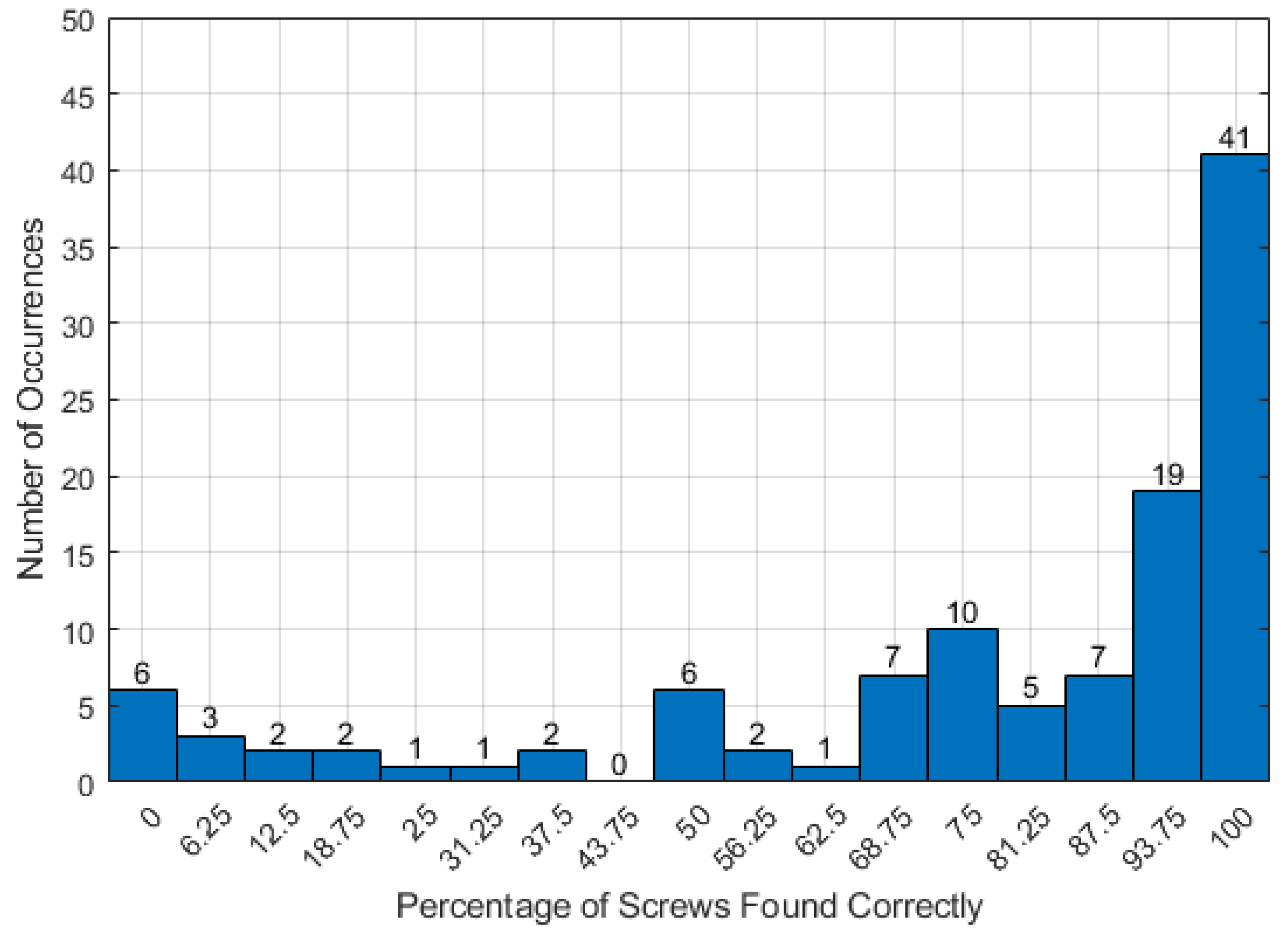
The results depicted in Figure 9 show the percentage at which the individual screws were detected over the 16 trials. For six screws, a 0% detection rate was recorded over all the trials, while 23 screws exhibited a detection rate of 50% or less. In contrast, 41 screws demonstrated a perfect detection rate, being identified 100% of the time. In terms of terminology, screws with a detection rate of 50% or lower were considered to have a “poor detection rate”, whereas screws consistently identified with a 100% rate were categorized as having a “perfect detection rate”.

Data collection for each of the seven laptops involved recording information for every screw across all trials, and these data were organized into a table format. For illustration, the table for GATE2 is presented in

Table 5. Expanded detection data for screws and false positives for Gate2.

Trial Groups
Detections
Screw #	V10 S15 S nl	V10 S15 S wl	V10 S15 XL nl	V10 S15 XL wl	V10 S25 S nl	V10 S25 S wl	V10 S25 XL nl	V10 S25 XL wl	V15 S15 S nl	V15 S15 S wl	V15 S15 XL nl	V15 S15 XL wl	V15 S25 S nl	V15 S25 S wl	V15 S25 XL nl	V15 S25 XL wl	Sum	Total %
1	0	0	1	1	1	1	1	1	0	0	1	1	0	0	1	1	10	62.5%
2	1	1	1	1	1	1	1	1	0	0	0	0	0	0	0	0	8	50.0%
3	1	1	1	1	1	1	1	1	1	1	1	1	0	1	1	1	15	93.8%
4	1	1	1	1	1	1	1	1	1	1	0	1	1	1	0	1	14	87.5%
5	1	1	1	1	1	1	1	1	1	1	1	1	1	1	1	1	16	100.0%
6	1	1	1	1	1	1	1	1	1	1	1	1	1	1	1	1	16	100.0%
7	1	1	1	1	1	1	1	1	1	1	1	1	1	1	1	1	16	100.0%
8	1	0	0	0	1	1	0	0	0	1	0	0	0	1	0	0	5	31.3%
9	1	1	1	1	1	1	1	1	1	1	1	1	1	1	1	1	16	100.0%
10	1	1	1	1	1	1	1	1	1	0	0	1	0	1	0	0	11	68.8%
11	1	1	1	1	1	1	1	1	1	1	1	1	1	1	1	1	16	100.0%
12	1	1	1	1	1	1	1	1	1	1	1	1	1	1	1	1	16	100.0%
13	1	1	1	1	1	1	1	1	1	1	1	1	1	1	1	1	16	100.0%
14	1	1	1	1	1	1	1	1	1	1	1	1	1	1	1	1	16	100.0%
15	1	1	1	1	1	1	1	1	1	1	1	1	1	1	1	1	16	100.0%
16	0	1	0	0	1	1	0	0	0	1	0	0	1	1	0	0	6	37.5%
17	1	1	1	1	1	1	1	1	1	1	1	0	1	1	1	1	15	93.8%
18	1	1	1	1	1	1	1	1	1	1	1	1	1	1	1	1	16	100.0%
19	0	0	0	1	0	0	0	0	0	0	0	1	0	0	0	0	2	12.5%
20	1	1	1	1	1	1	1	1	1	1	1	1	0	1	1	1	15	93.8%
21	1	1	1	1	1	1	1	1	0	1	1	1	1	1	1	1	15	93.8%
F1	0	1	0	0	0	0	0	0	0	0	0	0	0	0	0	0	1	6.3%
F2	0	1	0	0	0	0	0	0	1	0	0	0	0	1	0	0	3	18.8%
F3	0	0	0	0	0	1	0	0	0	0	0	0	0	0	0	0	1	6.3%
F4	0	0	0	0	0	0	0	0	0	0	0	0	0	1	0	0	1	6.3%
F5	1	0	0	0	0	0	0	0	0	0	0	0	0	0	0	0	1	6.3%
F6	0	0	0	0	0	0	0	0	1	0	0	0	0	0	0	0	1	6.3%

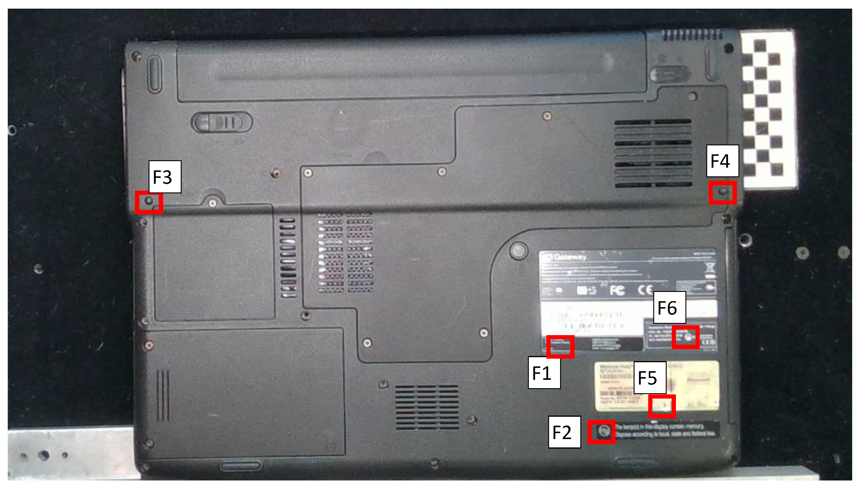
. The rows are organized by screw number, which corresponds to the screw numbers on the coordinate plot map of the laptop in Figure 5b. Rows F1 through F6 designate specific regions on the laptop where false detections were pinpointed, and they are shown in Figure 10. The regions of false detection for the other laptops can be found in S3-False Detection Regions.pdf in the Github repository. It should be noted that the number of regions found are not fixed; they varied between 6 for GATE2 and 21 for DELL1. Meanwhile, the columns of the chart were organized to represent individual trials, with a value of 0 indicating a missed detection and a value of 1 signifying a correct detection. The column “Sum” sums up all of the detections for an individual screw or false detection, and the column “Total %” is the sum total divided by the 16 trials. The data for the rest of the laptops can be found in S4-Screw Characteristics.xlsx in the Github repository in their corresponding worksheet.

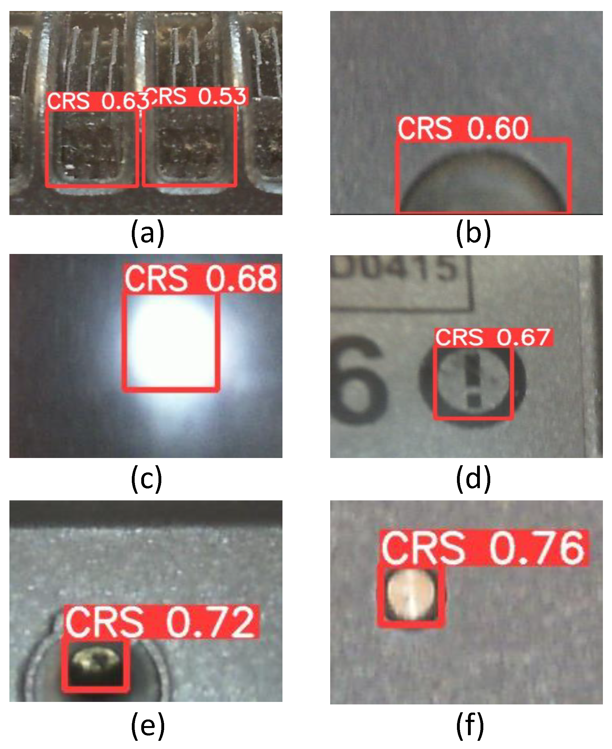
Utilizing the tables for all the laptops makes it feasible to categorize the false detections into six distinct groups. These groups include grates, protruding shapes, reflective surfaces, stickers, deep holes, and surface shapes or marks. Visual examples of each of these groups are shown in Figure 11, and the total number of detections and their percentages are tallied in

Table 6. False detections broken down by different categories.

Categories	Total Detections	Percent Detection Rate
Grate	42	14.44
Protruding shape	54	18.56
Reflective textures	5	1.72
Sticker	120	41.24
Deep hole	14	4.81
Surface shapes or marks	56	19.24
Total False Detections	291

. These numbers show that, over the 16 trials, there were 291 total false detections. Stickers were the cause of most of the false detections, while reflective textures and deep holes caused the least amount of false detections.

Table 7. Sample percentages and detection percentages of different screw groupings. The factors compared are (1) a deep/surface screw, (2) screws for which the hole has/does not have a taper, (3) screws with an exterior/interior/corner location, and (4) screws for which the color difference between the screw and the laptop was none/medium/large.

Categories	Poor Detection Rate Sample %	Perfect Detection Rate Sample %	All Screws Sample %	All Screws Detection Percentage
Deep screw	100	43.9	68.7	68.8
Surface screw	0.0	56.1	31.3	94.1
Has a taper	34.8	9.8	17.4	56.9
No taper	65.2	90.2	82.6	80.9
Exterior screw	60.9	31.7	40.0	69.8
Interior screw	21.7	51.2	38.3	85.2
Corner screw	17.4	17.1	21.7	74.3
Large color difference	26.1	29.3	26.1	80.0
Medium color difference	47.8	34.1	34.8	68.6
No color difference	26.1	36.6	39.1	81.7

offers a comprehensive breakdown of screw characteristics and their associated sample percentages. This table classifies screws based on specific attributes and then calculates the percentages within each attribute category. To illustrate, consider the “Deep Screw” row and the column labeled “Poor Detection Rate Sample %”. This calculates the percentage of screws classified as deep screws that also had a detection rate of 50% or less. This percentage is determined by dividing the number of screws meeting these criteria by the total count of screws with a detection rate under 50% (23 screws). For comparison, the “Surface Screw” row contained no screws classified as both surface screws and screws having a poor detection rate, resulting in a sample percentage of 0%. Consequently, the Deep Screw sample percentage is 100%. The “Perfect Detection Rate Sample %” column calculates the percentage of deep screws that achieved a 100% detection rate by dividing the number of screws meeting these criteria by the total count of screws with a 100% detection rate (41 screws). The “All Screws Sample %” column provides the overall percentage of deep screws in relation to the entire set of screws (115). Notably, this table ensures that the sample percentages within different categories (e.g., Deep Screw or Surface Screw, Has a Taper or No Taper, etc. ) sum up to 100%, independently of the other categories.

Finally, the “All Screws Detection Percentage” column presents the average detection percentage for screws of a particular category. The system was, on average, able to find 68.8% of all the deep screws and 94.1% of all the surface screws. One should note the reported percentage is not a vision-accuracy percentage because only correct detections were analyzed. This reported percentage represents the average percentage at which a particular screw was discovered across all the trials when the specified condition was satisfied. For example, the 94.1% value for surface screws came from taking the average of the “Total %” column in Table 5 for any screw classified as a surface screw over all the laptop models. This column shows how several characteristics significantly influence the ease of detecting screws. First, screws placed on the surface of an object were found to be more easily detectable than those buried deep within the material. Additionally, screws with a tapered shape proved to be more challenging to detect compared to their non-tapered counterparts. The location of the screws also played a role, with interior screws exhibiting a higher detection rate compared to screws situated at corners or on the exterior of objects. Interestingly, the color differentiation on the screws also impacts detection, as screws with a large color difference or no color difference at all were easier to spot than those with a medium color difference.

To better understand and view these screw characteristic sample percentages and breakdowns, the four screw characteristics were translated into binary data. All possible combinations were analyzed to view the effect that the four screw characteristics had on the screw detection within the data set. Characteristics associated with a high detection rates (surface screw, no taper, internal screws, and no color difference) were labeled as “1”, and characteristics with a negative association were labeled as “0”. In this analysis, corner screws were grouped with exterior screws. These groupings were selected based on the “All Screws Detection percentage” rates in Table 7. Each of these categories were then labeled with a letter. Depth was labeled as “A”, taper was labeled as “B”, position was labeled as “C”, and color difference was labeled as “D”. Each of these characteristics was combined to get all of the possible combinations of screw characteristics. The Venn diagram shown in Figure 12, shows the percentage detection for the different combinations. These results show that of all the combinations, the system had the best detection rates when a screw was a surface screw, regardless of its other characteristics. The data for the Venn diagram can be viewed in the S4-Screw Characteristics in the Binary Data Expanded tab.

4. Discussion

To achieve accurate automatic screw detection in a robotic system with a neural network, various factors come into play. One crucial consideration involves the velocity at which the robot collects data. If the robot moves too quickly, it can lead to blurred features that are hard to discern. Conversely, if the machine moves too slowly, a very large number of images are generated, and there is an increased risk of false detections from one of the categories referred to in Table 6. The paper identifies an optimal medium velocity range of 10 to 15 mm/s, which yielded the best results. Another important factor pertains to the collection of data and the use of external lighting to illuminate the area, particularly when working with laptops. Interestingly, the effectiveness of this parameter is laptop-dependent. In most cases, employing additional light enhances vision accuracy. However, on select laptops, it can result in more false detections, thus diminishing accuracy. Notably, laptops with lighter-colored cases tend to suffer from reduced accuracy when external lighting is used, whereas laptops with darker cases benefit from the added illumination. Lastly, the number of passes the robot makes over the laptop does not impact the detection accuracy of the system.

Table 8. Screw detection comparison with other work. TD = true detections, FD = false detections, and T = total number of screws.

Reported Work	Types of Screws Detected	Reported Accuracy	Accuracy Metric Used
This work	Cross-recessed screws on the back of laptops	Average over all trial groups up to 73.4%, Individual trials up to 95% laptop- and parameter-dependent	${\displaystyle \frac{TD-FD}{T}}$
DiFilippo and Jouaneh [22]	Cross-recessed screws on the back of laptops	Up to 86.7% dependent on laptop color and camera settings	${\displaystyle \frac{TD}{T}}$
Foo et al. [45]	Crosshead screws on components of LCD monitors	Up to 78%, depending on scenario.	${\displaystyle \frac{TD}{T+FD}}$
Li et al. [46]	Hex screws and cross screws on mobile phone boards	>97% in test cases	${\displaystyle \frac{TD}{T}}$
Mangold et al. [47]	Six screw heads—Pozidriv, hex-socket, slot-drive, Phillips (cross-recessed), hex, and Torx on motors	86% small-motor and 88% large-motor	${\displaystyle \frac{TD}{T}}$

presents the results of this study’s screw detection compared to other works. Direct comparison is challenging due to the different accuracy metrics used in these papers. For instance, DiFilippo and Jouaneh [22], Mangold et al. [47], and Li et al. [46] reported accuracy as the ratio of correctly detected screws to the total screws, without penalizing false detections. If false detections were accounted for, their reported accuracies would be lower. Foo et al. [45] employed an accuracy metric that included false detections similar to the one used in this paper, but false detections were added to the total number of screws. Our method goes further by penalizing false detections more severely, subtracting them from the count of true detections across all trials. When using the accuracy metric from [45], our reported percentages would remain the same or increase.

A critical parameter tested in the neural network is the network size, which played a crucial role in vision accuracy. Larger networks generally led to better accuracy; however, they also came with the trade-off of increased computational demands and longer processing times. The accuracy of neural networks in detecting screws is significantly influenced by various screw characteristics, such as color and taper. In summary, the system showed a higher accuracy in identifying screws that fall into certain categories. These include screws on the laptop’s surface, screws without a taper, interior screws, and screws and laptop cases with a significant color difference or no color difference at all. Upon closer examination of the data, screws with a lower detection rate tended to have an average depth of approximately 0.351" (about 8.9 mm), whereas screws with a perfect detection rate had an average depth of approximately 0.105" (about 2.7 mm).

When examining screw locations, it becomes evident that exterior screws posed a more significant challenge for the neural network’s detection capabilities. They accounted for 60.9% of the screws in the poor detection category while comprising only 31.7% of the screws in the perfect detection category. In contrast, corner screws showed relatively consistent detection rates between the two categories, 17.4% and 17.1%, respectively, suggesting that their location did not significantly impact detection outcomes. Interior screws, on the other hand, exhibited a noteworthy difference in detection rates. They were more prevalent in the perfect detection category (51.2%) compared to the poor detection category (21.7%), indicating that the neural network was better at detecting interior screws than exterior ones. Additionally, when examining screws with a taper, all 20 of them were categorized as deep screws. Furthermore, 19 out of these 20 screws were located either on the laptop’s exterior or in corner positions that were already shown to be more difficult to detect.

When analyzing the number of false detections over all trials, DELL1 and GATE2 had the highest false detection counts (207 and 173, respectively). When the data were limited to just trials at 10 and 15 mm/s, the two laptops with the highest false detection counts were DELL1 and FUJI1 with 81 and 69 false detections. Looking at these false detections in further detail reveals that, on the FUJI1 laptop, various surface marks and shapes comprised 28 false detections, and 19 false detections were categorized as stickers. In comparison, the DELL1 had 65 false detections that were categorized as stickers, specifically various circular shapes and images found on the stickers from third-party certifications.

5. Conclusions

In conclusion, screw detection plays a vital role in automating the disassembly process, as screws are one of the most commonly used fasteners. Overall, neural networks present an attractive method for fastener detection due to how quickly they can process an image compared to traditional computer vision methods and the availability of tools used to train them. However, it is important to acknowledge that screw detection remains a significant challenge due to the diverse array of configurations in which screws can be employed.

The objective of this study was to determine the optimal operational parameters for a robotic system when acquiring and analyzing images to detect cross-recessed screws on laptops using a YOLOv5 neural network. It was shown that various factors impact the performance of a robotic system when it comes to screw detection with a neural network. During the data analysis phase, two critical factors emerged as significant: the velocity at which the robot moved and the use of external lighting. Specifically, the best results were achieved when employing a Cartesian robot moving at velocities of either 10 or 15 mm/s and using external lighting for laptops with dark colors and no additional lighting for laptops with lighter colors. When it comes to analyzing images with a neural network, the size of the neural network architecture is important. Notably, a larger neural network, YOLOv5-XL, outperformed a smaller one and resulted in higher detection accuracy. The characteristics of individual screws also impact the system’s ability to detect them accurately. The system performed best with screws located on the laptop’s surface, without a taper, and positioned away from the laptop’s edges. The results also show that the highest detection level occurred with either a large color difference or no color difference between the screws and the laptop case. However, the most critical factor influencing accurate screw detection was found to be the depth at which the screw was recessed into the laptop. A factor that did not have a notable effect on the screw detection accuracy was the number of passes the robot made over the laptop.

In future research, the focus will be on enhancing the accuracy and reliability of screw detection by implementing measures to reduce false detections. This includes developing advanced filtering techniques to distinguish true detections from false positives, ultimately increasing confidence in the accuracy of detected screws. Furthermore, an exploration of methods to improve the detection of screws recessed into deeper holes, potentially by experimenting with brighter lighting conditions beneath the camera or exploring alternative sensor technologies, such as depth sensors, that can provide better visibility in such scenarios, will be pursued. Additionally, efforts will be made to assess the processing time and hardware demands, particularly in the context of large-scale e-waste applications. These efforts will aim to advance the capabilities of the robotic system and make it more robust in detecting screws in a wider range of challenging conditions.

References

- Shahabuddin, M.; Uddin, M.N.; Chowdhury, J.I.; Ahmed, S.F.; Uddin, M.N.; Mofijur, M.; Uddin, M.A. A review of the recent development, challenges, and opportunities of electronic waste (e-waste). Int. J. Environ. Sci. Technol. 2023, 20, 4513–4520. [Google Scholar] [CrossRef]
- Forti, V.; Balde, C.P.; Kuehr, R.; Bel, G. The Global E-Waste Monitor 2020: Quantities, Flows and the Circular Economy Potential; Technical report; United Nations University (UNU)/United Nations Institute for Training and Research (UNITAR)—Co-Hosted SCYCLE Programme, International Telecommunication Union (ITU) & International Solid Waste Association: Bonn, Germany; Geneva, Switzerland; Rotterdam, The Netherlands, 2020; Available online: https://ewastemonitor.info/gem-2020 (accessed on 9 July 2024).
- E-Waste. Vol. 1: Inventory Assessment Manual. Technical Report, United Nations Environment Programme 2007. Available online: https://wedocs.unep.org/20.500.11822/7857 (accessed on 9 July 2024).
- Widmer, R.; Oswald-Krapf, H.; Sinha-Khetriwal, D.; Schnellmann, M.; Böni, H. Global perspectives on e-waste. Environ. Impact Assess. Rev. 2005, 25, 436–458. [Google Scholar] [CrossRef]
- United Nations Environment Programme. Basel Convention: Controlling Transboundary Movements of Hazardous Wastes and Their Disposal. Available online: https://www.basel.int/Implementation/Ewaste/Overview/tabid/4063/Default.aspx. (accessed on 12 July 2024).
- European Parliament and Council. Regulation (EU) 2024/1157 of the European Parliament and of the Council of 11 April 2024 on shipments of waste, amending Regulations (EU) No 1257/2013 and (EU) 2020/1056 and repealing Regulation (EC) No 1013/2006. Off. J. Eur. Union 2024. Available online: http://data.europa.eu/eli/reg/2024/1157/oj (accessed on 16 July 2024).
- Lin, S.; Man, Y.B.; Chow, K.L.; Zheng, C.; Wong, M.H. Impacts of the influx of e-waste into Hong Kong after China has tightened up entry regulations. Crit. Rev. Environ. Sci. Technol. 2020, 50, 105–134. [Google Scholar] [CrossRef]
- Liu, K.; Tan, Q.; Yu, J.; Wang, M. A global perspective on e-waste recycling. Circ. Econ. 2023, 2, 100028. [Google Scholar] [CrossRef]
- Hashmi, M.Z.; Chen, K.; Khalid, F.; Yu, C.; Tang, X.; Li, A.; Shen, C. Forty years studies on polychlorinated biphenyls pollution, food safety, health risk, and human health in an e-waste recycling area from Taizhou city, China: A review. Environ. Sci. Pollut. Res. 2021, 29, 4991–5005. [Google Scholar] [CrossRef] [PubMed]
- Orisakwe, O.E.; Frazzoli, C.; Ilo, C.E.; Oritsemuelebi, B. Public health burden of e-waste in Africa. J. Health Pollut. 2019, 9, 190610. [Google Scholar] [CrossRef]
- Herat, S. E-waste management in Asia Pacific region: Review of issues, challenges and solutions. Nat. Environ. Pollut. Technol. 2021, 20, 45–53. [Google Scholar] [CrossRef]
- Nnorom, I.C.; Osibanjo, O. Overview of electronic waste (e-waste) management practices and legislations, and their poor applications in the developing countries. Resour. Conserv. Recy. 2008, 52, 843–858. [Google Scholar] [CrossRef]
- Kumar, A.; Holuszko, M.; Espinosa, D.C.R. E-waste: An overview on generation, collection, legislation and recycling practices. Resour. Conserv. Recycl. 2017, 122, 32–42. [Google Scholar] [CrossRef]
- Foo, G.; Kara, S.; Pagnucco, M. Challenges of robotic disassembly in practice. Procedia CIRP 2022, 105, 513–518. [Google Scholar] [CrossRef]
- Duflou, J.R.; Seliger, G.; Kara, S.; Umeda, Y.; Ometto, A.; Willems, B. Efficiency and feasibility of product disassembly: A case-based study. CIRP Ann. 2008, 57, 583–600. [Google Scholar] [CrossRef]
- Bogue, R. Robots in recycling and disassembly. Ind. Rob. 2019, 46, 461–466. [Google Scholar] [CrossRef]
- Vongbunyong, S.; Kara, S.; Pagnucco, M. Learning and revision in cognitive robotics disassembly automation. Robot. Comput. Integr. Manuf. 2015, 34, 79–94. [Google Scholar] [CrossRef]
- Vongbunyong, S.; Kara, S.; Pagnucco, M. General plans for removing main components in cognitive robotic disassembly automation. In Proceedings of the 2015 6th International Conference on Automation, Robotics and Applications, Queenstown, New Zealand, 17–19 February 2015; IEEE: Queenstown, New Zealand, 2015; pp. 501–506. [Google Scholar] [CrossRef]
- Vongbunyong, S.; Kara, S.; Pagnucco, M. Application of cognitive robotics in disassembly of products. CIRP Ann. 2013, 62, 31–34. [Google Scholar] [CrossRef]
- Foo, G.; Kara, S.; Pagnucco, M. An ontology-based method for semi-automatic disassembly of LCD monitors and unexpected product types. Int. J. Autom. Technol. 2021, 15, 168–181. [Google Scholar] [CrossRef]
- Foo, G.; Kara, S.; Pagnucco, M. Artificial Learning for Part Identification in Robotic Disassembly Through Automatic Rule Generation in an Ontology. IEEE Trans. Autom. Sci. Eng. 2022, 20, 296–309. [Google Scholar] [CrossRef]
- DiFilippo, N.M.; Jouaneh, M.K. A system combining force and vision sensing for automated screw removal on laptops. IEEE Trans. Autom. Sci. Eng. 2017, 15, 887–895. [Google Scholar] [CrossRef]
- DiFilippo, N.M.; Jouaneh, M.K. Using the soar cognitive architecture to remove screws from different laptop models. IEEE Trans. Autom. Sci. Eng. 2018, 16, 767–780. [Google Scholar] [CrossRef]
- Li, R.; Pham, D.T.; Huang, J.; Tan, Y.; Qu, M.; Wang, Y.; Kerin, M.; Jiang, K.; Su, S.; Ji, C.; et al. Unfastening of hexagonal headed screws by a collaborative robot. IEEE Trans. Autom. Sci. Eng. 2020, 17, 1455–1468. [Google Scholar] [CrossRef]
- Chen, J.; Liu, Z.; Xu, J.; Yang, C.; Chu, H.; Cheng, Q. A Novel Disassembly Strategy of Hexagonal Screws Based on Robot Vision and Robot-Tool Cooperated Motion. Appl. Sci. 2022, 13, 251. [Google Scholar] [CrossRef]
- Klas, C.; Hundhausen, F.; Gao, J.; Dreher, C.R.; Reither, S.; Zhou, Y.; Asfour, T. The KIT gripper: A multi-functional gripper for disassembly tasks. In Proceedings of the 2021 IEEE International Conference on Robotics and Automation, Xi’an, China, 30 May 2021–5 June 2021; IEEE: Xi’an, China, 2021; pp. 715–721. [Google Scholar] [CrossRef]
- On Robot—Multifunctional Robot Screwdriver with Screwfeeder. Available online: https://onrobot.com/us/products/onrobot-screwdriver (accessed on 12 July 2024).
- Atlas Copco—Fixed Current Control Screwdriver QMC. Available online: https://www.atlascopco.com/en-us/itba/products/fixtured-current-controlled-screwdriver%C2%A0qmc-sku4397 (accessed on 12 July 2024).
- Peeters, J.R.; Vanegas, P.; Mouton, C.; Dewulf, W.; Duflou, J.R. Tool design for electronic product dismantling. Procedia CIRP 2016, 48, 466–471. [Google Scholar] [CrossRef]
- Figueiredo, W. A High-Speed Robotic Disassembly System for the Recycling and Reuse of Cellphones. Master’s Thesis, Massachusetts Institute of Technology, Cambridge, MA, USA, 2018. [Google Scholar]
- Schumacher, P.; Jouaneh, M. A system for automated disassembly of snap-fit covers. Int. J. Adv. Manuf. Tech. 2013, 69, 2055–2069. [Google Scholar] [CrossRef]
- Schumacher, P.; Jouaneh, M. A force sensing tool for disassembly operations. Robot. Comput. Integr. Manuf. 2014, 30, 206–217. [Google Scholar] [CrossRef]
- Gil, P.; Pomares, J.; Diaz, S.v.P.C.; Candelas, F.; Torres, F. Flexible multi-sensorial system for automatic disassembly using cooperative robots. Int. J. Comput. Integr. Manuf. 2007, 20, 757–772. [Google Scholar] [CrossRef]
- Büker, U.; Drüe, S.; Götze, N.; Hartmann, G.; Kalkreuter, B.; Stemmer, R.; Trapp, R. Vision-based control of an autonomous disassembly station. Rob. Auton. Syst. 2001, 35, 179–189. [Google Scholar] [CrossRef]
- Bdiwi, M.; Rashid, A.; Putz, M. Autonomous disassembly of electric vehicle motors based on robot cognition. In Proceedings of the 2016 IEEE International Conference on Robotics and Automation, Stockholm, Sweden, 16–21 May 2016; IEEE: Stockholm, Sweden, 2016; pp. 2500–2505. [Google Scholar] [CrossRef]
- Zhao, Z.Q.; Zheng, P.; Xu, S.t.; Wu, X. Object detection with deep learning: A review. IEEE Trans. Neural Netw. Learn. Syst. 2019, 30, 3212–3232. [Google Scholar] [CrossRef] [PubMed]
- Krizhevsky, A.; Sutskever, I.; Hinton, G.E. Imagenet classification with deep convolutional neural networks. Adv. Neural Inf. Process. Syst. 2012, 25, 84–90. [Google Scholar] [CrossRef]
- Ren, S.; He, K.; Girshick, R.; Sun, J. Faster r-cnn: Towards real-time object detection with region proposal networks. IEEE Trans. Pattern Anal. Mach. Intell. 2015, 28, 1137–1149. [Google Scholar] [CrossRef]
- Redmon, J.; Divvala, S.; Girshick, R.; Farhadi, A. You only look once: Unified, real-time object detection. In Proceedings of the IEEE Conference on Computer Vision and Pattern Recognition, Las Vegas, NV, USA, 27–30 June 2016; IEEE: Las Vegas, NV, USA, 2016; pp. 779–788. [Google Scholar] [CrossRef]
- Liu, W.; Anguelov, D.; Erhan, D.; Szegedy, C.; Reed, S.; Fu, C.Y.; Berg, A.C. SSD: Single shot multibox detector. In Proceedings of the Computer Vision–ECCV 2016, Amsterdam, The Netherlands, 11–14 October 2016; Springer: Amsterdam, The Netherlands, 2016; pp. 21–37. [Google Scholar] [CrossRef]
- Wu, X.; Sahoo, D.; Hoi, S.C. Recent advances in deep learning for object detection. Neurocomputing 2020, 396, 39–64. [Google Scholar] [CrossRef]
- Yildiz, E.; Wörgötter, F. DCNN-based screw detection for automated disassembly processes. In Proceedings of the 2019 15th International Conference on Signal-Image Technology & Internet-Based Systems, Sorrento, Italy, 26–29 November 2019; IEEE: Sorrento, Italy, 2019; pp. 187–192. [Google Scholar] [CrossRef]
- Yildiz, E.; Wörgötter, F. DCNN-based Screw Classification in Automated Disassembly Processes. In Proceedings of the International Conference on Robotics, Computer Vision and Intelligent Systems, Online, 4–6 November 2020; pp. 61–68. [Google Scholar] [CrossRef]
- Brogan, D.P.; DiFilippo, N.M.; Jouaneh, M.K. Deep learning computer vision for robotic disassembly and servicing applications. Array 2021, 12, 100094. [Google Scholar] [CrossRef]
- Foo, G.; Kara, S.; Pagnucco, M. Screw detection for disassembly of electronic waste using reasoning and re-training of a deep learning model. Procedia CIRP 2021, 98, 666–671. [Google Scholar] [CrossRef]
- Li, X.; Li, M.; Wu, Y.; Zhou, D.; Liu, T.; Hao, F.; Yue, J.; Ma, Q. Accurate screw detection method based on faster R-CNN and rotation edge similarity for automatic screw disassembly. Int. J. Comput. Integr. Manuf. 2021, 34, 1177–1195. [Google Scholar] [CrossRef]
- Mangold, S.; Steiner, C.; Friedmann, M.; Fleischer, J. Vision-based screw head detection for automated disassembly for remanufacturing. Procedia CIRP 2022, 105, 1–6. [Google Scholar] [CrossRef]
- Zhang, X.; Eltouny, K.; Liang, X.; Behdad, S. Automatic Screw Detection and Tool Recommendation System for Robotic Disassembly. J. Manuf. Sci. Eng. 2023, 145, 031008. [Google Scholar] [CrossRef]
- Peralta, P.E.; Ferre, M.; Sánchez-Urán, M.Á. Robust Fastener Detection Based on Force and Vision Algorithms in Robotic (Un) Screwing Applications. Sensors 2023, 23, 4527. [Google Scholar] [CrossRef] [PubMed]
- Liu, Q.; Deng, W.; Pham, D.T.; Hu, J.; Wang, Y.; Zhou, Z. A Two-Stage Screw Detection Framework for Automatic Disassembly Using a Reflection Feature Regression Model. Micromachines 2023, 14, 946. [Google Scholar] [CrossRef]
- Li, H.; Zhang, H.; Zhang, Y.; Zhang, S.; Peng, Y.; Wang, Z.; Song, H.; Chen, M. An Accurate Activate Screw Detection Method for Automatic Electric Vehicle Battery Disassembly. Batteries 2023, 9, 187. [Google Scholar] [CrossRef]
- Peta, K.; Żurek, J. Prediction of air leakage in heat exchangers for automotive applications using artificial neural networks. In Proceedings of the 2018 9th IEEE Annual Ubiquitous Computing, Electronics & Mobile Communication Conference, New York, NY, USA, 8–10 November 2018; IEEE: New York, NY, USA, 2018; pp. 721–725. [Google Scholar] [CrossRef]
- Ultralytics YOLOv5 Architecture. Available online: https://docs.ultralytics.com/yolov5/tutorials/architecture_description/ (accessed on 12 July 2024).
Figure 1.
(a) Setup of the robotic system with a laptop from a front view and the robot at its home position. (b) Top down view of the workspace, showing a laptop and the spacer used to offset the laptops so that the home position aligns with the mounted camera.
Figure 2.
The backs of all the laptops tested in the trials. The laptops were identified according to their manufacturers (Compaq, Dell, Gateway, HP, and Fujitsu) and a number.
Figure 3.
The movement pattern performed by the robot during trials.
Figure 4.
The coordinate system of different subsystems used for trial testing. These are shown when the robot is at its home position. The spacer and offsets allow for the camera to cover the entire laptop.
Figure 5.
(a) A coordinate map showing the detected screws as blue circles and the actual screw locations as orange screws on the GATE2 laptop. It should be noted that these circles were enlarged to improve visibility in the image. (b) An image of the GATE2 laptop with screws that are highlighted in red and numbered to correspond with the numbers in the coordinate map.
Figure 6.
An output image from the neural network, highlighting a detected screw within a bounding box. The value displayed within the bounding box, in this case, 0.91, represents the confidence score assigned via the neural network. This score quantifies the network’s certainty that the identified object is indeed a screw, with values ranging from 0.0 (no confidence) to 1.0 (complete confidence).
Figure 7.
Vision accuracy percentage results across all trials broken down by laptop.
Figure 8.
Vision accuracy percentage for four different trials broken down by laptop.
Figure 9.
Number of occurrences where an individual screw was detected over all trials grouped according to percentages.
Figure 10.
Locations of the false detections on the GATE2 laptop labeled F1–F6. Here F1, F2, F5, and F6 are classified as stickers, and F3 and F4 are classified as protruding shapes.
Figure 11.
Different examples of categories the system found. Note that these images were cropped for visibility. (a) grates; (b) protruding shape; (c) reflective surface; (d) sticker; (e) deep hole; and (f) surface shapes or marks.
Figure 12.
Venn diagram showing combinations of screw characteristics and their corresponding screw detection rate. A—surface screw, B—no taper, C—interior screws, and D—no laptop or screw color difference.