POLIDriving: A Public-Access Driving Dataset for Road Traffic Safety Analysis

Abstract

The problems with current driving datasets are their exclusivity to autonomous driving applications and their limited diversity in terms of sources of information and number of attributes. Thus, this paper presents a novel driving dataset that contains information from several heterogeneous sources and targets road traffic safety applications. We used an acquisition module based on software and hardware to collect information from a vehicle scanner and a health monitor. This module also consumes information from a weather web service and databases on traffic accidents and road geometric characteristics. For the acquisition sessions, drivers of different ages and genders drove vehicles on two routes at different day hours in different weather conditions. POLIDriving contains around 18 h of driving data, more than 61k observations, and 32 attributes. Unlike the other related datasets that include information on vehicle and road conditions, POLIDriving also includes information on the driver, weather conditions, traffic accidents, and road geometric characteristics. The dataset was tested in learning models to predict the risk levels of suffering a traffic accident. Hence, we built two learning models: Gradient Boosting Machine (GBM) and Multilayer Perceptron (MLP). GBM reached an accuracy value of 95.6%, and MLP reached an accuracy of 98.6%. Undoubtedly, POLIDriving will contribute greatly to the research on traffic accident prevention by providing a novel, numerous, and diverse driving dataset.

1. Introduction

Determining the real cause of a traffic accident is complicated because there is often not enough information at the time. Generally, the cause is attributed to the driver’s carelessness or negligence; however, the real cause can be another or a combination of other factors. The Global Status Report of Road Safety [1] from the World Health Organization (WHO) focuses only on five key risk factors, leaving other factors aside. For instance, a real cause of an accident can be a mechanical failure of the vehicle, adverse weather conditions, poor design of the road, or, much worse, a combination of some of them. While more information is available, determining the real cause of an accident will be easier.

In traffic accident prevention, specifically in the research area of traffic accident prediction, it is essential to count with a driving dataset that correlates and integrates information from heterogeneous sources. According to Marcillo et al. [2], the data sources commonly used in this area are driver’s data, vehicle data, weather conditions, traffic accidents, traffic flow, traffic events, light conditions, and road infrastructure. Thus, the key to a new driving dataset targeted to this area is the inclusion of information from most of these sources.

There are great driving datasets such as A2D2 [3], KITTI [4], BDD100K [5], or Apollo Scape [6]; however, most of them target autonomous driving applications. There are also datasets such as comma.ai [7] or comma2k19 [8] that target autonomous driving and road safety applications, but these datasets include information from one or at most two sources. Vehicular traffic flow and accident prevention applications require driving datasets that include as much information as possible from various sources. Considering that our work focuses on traffic accident prevention, specifically in predicting risk levels of suffering a traffic accident, generating a driving dataset that fulfills the requirements of this type of application is essential.

Our main contribution is to provide the research community with a driving dataset that correlates and integrates information from heterogeneous sources. Through POLIDriving, we provide 15 h of driving data from five real drivers and three extra hours of synthetic driving data from a fake driver with risky driving behavior. We also describe the process of data labeling through semi-supervised and ensemble learning. Finally, we provide two supervised learning models to predict risk levels of suffering a traffic accident.

The rest of this article is organized as follows: Section 2 presents related driving datasets, Section 3 describes the process of generating the POLIDriving dataset, Section 4 presents the results of this work, Section 5 discusses the most relevant implications of the dataset, and Section 6 presents the conclusions of this work.

2. Related Work

We found driving datasets for autonomous driving and driving behavior upon review. Generally, they provide high-resolution images, distance and proximity measures, vehicle parameters, and geolocation. Considering that the target of POLIDriving is the identification of risky driving patterns, we have considered the datasets that provide mainly vehicle data and geolocation. Thus, according to these requirements, the following are the most relevant driving datasets.

COMMA.AI [7] is a 7-h driving dataset that contains images of the road and measures of sensors. This dataset includes the driving records of three drivers using one vehicle. It was generated using a frontal camera, a Light Detection and Ranging (LiDAR) sensor, and a Positioning and Orientation System (POS). Pictures were taken at 20 Hz, and the measures were integrated at 100 Hz. COMMA.AI includes information on the vehicle through the measurements of the sensors and the road conditions through the pictures of the road.

COMMA2K19 [8] is a 33-h driving dataset that contains road and in-vehicle images and measurements of sensors. This dataset includes the driver record of one driver using two vehicles. It was generated using a set of cameras (two frontal and one internal), an On-Board Diagnostics (OBD)-II scanner, a Global Navigation Satellite System (GNSS) receiver, and a 9-axis Inertial Measurement Unit (IMU). Pictures were taken at 20 Hz and the measurements at 100 Hz. COMMA2K19 includes information on vehicle and road conditions.

PREVENTION [9] is a 6-h driving dataset that contains front and rear images of the road and measurements of sensors. This dataset includes the driving records of three drivers using one vehicle. It was generated using two high-resolution cameras (one frontal and one rear-facing), a LiDAR sensor, three long-range radars (one narrow-field and two broad-field), a GNSS receiver, and a Controller Area Network (CAN) bus scanner. PREVENTION includes information on vehicle and road conditions.

AUTOMOTIVE OBD-II [10] is a 6-h driving dataset containing sensor measures. This dataset includes the driving record of ten vehicles. It was generated using only an OBD-II scanner and a mobile app. Sensor measurements were taken at 10 Hz. AUTOMOTIVE OBD-II includes only information on the vehicle such as engine coolant temperature, rpm, speed, throttle position (It monitors the position of the throttle valve that later controls the air entering the engine.), intake air temperature, and others.

A2D2 [3] is a driving dataset that contains images from six cameras and measurements of sensors. It contains 392.556 observations (frames) and each frame contains images and data files. A2D2 contains the driving record of one driver using one vehicle. It was generated using six cameras, six LiDAR sensors, one bus scanner, and one Global Positioning System (GPS) receiver. A2D2 includes information on vehicle and road conditions.

In contrast, we present POLIDriving, an 18-h driving dataset that includes information related to the driver, vehicle, weather conditions, traffic accidents, and road geometrics characteristics. It includes information from drivers of different ages and genders, with or without medical conditions or traffic violations, and information from vehicles of different brands, models, types, and years of fabrication. POLIDriving differs from other datasets in the number of drivers, vehicles, and data sources used for the data generation.

Table 1. Datasets features—Part 1.

Authors	Name	Duration	Frequency of  Acquisition	Drivers	Vehicles	Sensors/Devices	Applications
		[h]	[Hz]				Auton. Driving	Driving Behavior
Santana et al. [7]	comma.ai	7.25	pictures at 20 and measures at 100	3	1	1 frontal camera, 1 LiDAR sensor, and 1 POS device	✔	✔
Shafer et al. [8]	comma2k19	33	pictures at 20 and measures at 10	1	2	2 frontal cameras, 1 internal camera, 1 OBD-II scanner, 1 GNSS receiver, and 1 9-axis IMU device	✔	✔
Izquierdo et al. [9]	PREVENTION	6	laser at 10, radars at 33, and location receiver at 20	3	1	1 frontal camera, 1 rear-facing camera, 1 LiDAR sensor, 3 long-range radars, 1 GNSS receiver, and 1 CAN bus scanner	✔	✔
Weber et al. [10]	AUTOMOTIVE OBD-II	6	measures at 10	1	10	1 OBD-II scanner	-	✔
Geyer et al. [3]	A2D2	-	not mentioned	1	1	6 cameras, 6 LiDAR sensors, 1 GPS, 1 IMU, and 1 bus scanner	✔	✔
Marcillo et al.	POLIDriving	18	measures at 1	5	4	1 OBD-II scanner, 1 GPS receiver, and 1 health monitor	-	✔

and

Table 2. Datasets features—Part 2.

Name			Datasources				No. Attributes	Data Labeling	No. Classes
	Driver’s Data	Vehicle Data	Weather Conditions	Traffic Accidents	Geometric Charact.	Road Conditions
comma.ai	-	✔	-	-	-	✔ 1	40	-	-
comma2k19	-	✔	-	-	-	✔ 1	≈45	-	-
PREVENTION	-	✔	-	-	-	✔ 1	31	✔	-
AUTOMOTIVE OBD-II	-	✔	-	-	-	-	11	-	-
A2D2	-	✔	-	-	-	✔ 1	22	-	-
POLIDriving	✔	✔	✔	✔	✔	-	32	✔ 2	4

¹ pictures of the road. ² a part of the dataset.

present the features of the reviewed driving datasets.

3. Materials and Methods

This section presents the design of the acquisition module and the driver profiles, vehicles, devices, and services used in the acquisition sessions. Additionally, it presents the data sources and attributes included in the dataset, the selection of routes, and the geolocation of control points.

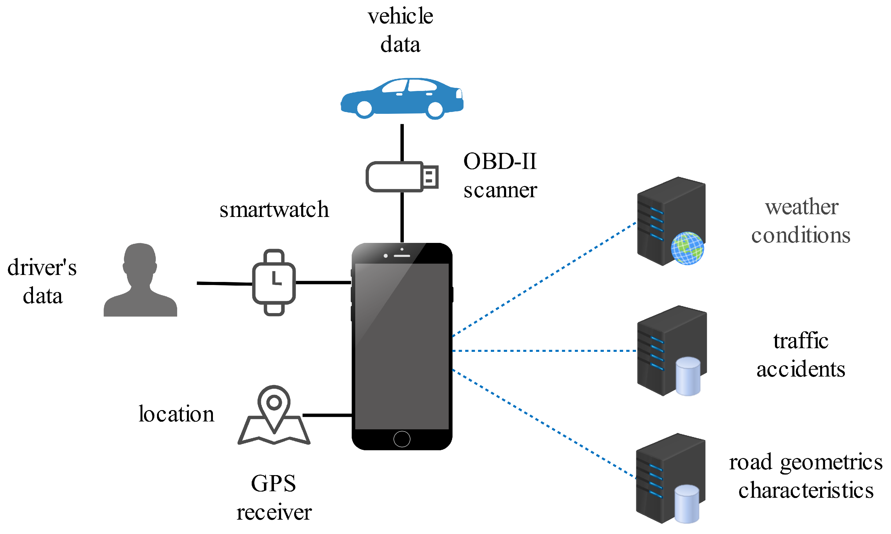
3.1. Acquisition Module

An acquisition module based on software and hardware was built to generate the driving dataset. This module consists of a mobile app that works with an OBD-II vehicle scanner, a GPS receiver, and a health monitor. Some vehicle parameters and the vehicle location are taken from the vehicular scanner and the geolocation device through the mobile app. Additionally, this module consists of software used to consume information from a weather service and to get information from a traffic accident database, a road geometrics database, and a health monitor. The weather conditions are taken from the weather service, the number of deaths from the traffic accidents database, the design speeds from the road geometrics characteristics database, and some health parameters of the driver from the health monitor. Figure 1 presents the design of the acquisition module.

3.2. Drivers and Vehicles

The following driver profiles and vehicles were used in this experiment.

• One woman and four men between 25 and 43 years old of different body constitutions, with or without medical conditions, traffic violations, and driving experience.
• Cross-Over Utility Vehicle (CUV), PICKUP, SEDAN-type vehicles of different brands, models, and different years of fabrication.

Table 3. Drivers’ information.

ID	Name	Gender	Age [Years]	Weight [kg]	Height [cm]	Medical Conditions	Driver’s License Points [/30]	Driving Experience [Years]
1	Pablo	Male	40	59	165	None	30	13
2	Andres	Male	25	69	163	None	30	7
3	Richard	Male	37	74	170	None	30	19
4	Alonso	Male	43	77	170	None	30	20
5	Yolanda	Female	43	62	155	None	30	23

and

Table 4. Vehicles information.

ID	Brand	Model	Type	Year Manufacture	Kilometers Travelled [×1000]	Last Maintenance [Year]	Number Airbags
1	Kia	Sportage	CUV	2018	31	2023	2
2	Kia	Soluto	Sedan	2022	75	2022	2
3	Chevrolet	DMAX	Pickup	2013	350	2023	2
4	Chevrolet	Cavalier	Sedan	2018	160	2021	2

present information on the drivers and vehicles.

3.3. Devices and Services

We equipped the vehicles used in the acquisition sessions with Veepeak OBDCheck BLE [11] scanners and Android cellphones, and their drivers wore Garmin Vivosmart 5 [12] health monitors. OBDCheck BLE is a vehicular scanner built on Bluetooth technology with support for OBD-II protocols such as CAN [13], KWP2000 [14], ISO9141-2 [15], J1850 VPW [16], and J1850 PWM [16]. The vehicular scanner receives measures from different Electronic Control Units (ECU (It is an embedded system that controls electrical systems in a vehicle. Many ECUs form the vehicle computer.)) every 100 ms, which are then merged to obtain observations at 1 Hz. Vivosmart 5 is a health monitor built on sensors that permits obtaining parameters such as heart rate, body temperature, body battery, and stress level.

The acquisition module uses the Accuweather service [17] to obtain weather information, a remote database from the Transit National Agency (ANT) [18] to obtain traffic accidents, and an own database (Section 3.6) to obtain road geometric characteristics. The Accuweather service provides weather conditions for a specific location each hour. The Locations API obtains a location key, which the CurrentConditions API uses to obtain the current conditions through a JSON object. Based on historical information about traffic accidents, the acquisition module determines the number of accidents around a specific location. Similarly, it determines the safe speed (design speed) in a specific location using the closest distance to the control points.

3.4. Data Sources and Attributes

Based on these studies [2,19,20], we chose the most relevant data sources and attributes for POLIDriving. Thus, our dataset contains information from different data sources, such as driver, vehicle, weather conditions, traffic accidents, and road geometric characteristics. Related to the attributes of each data source, the vehicle data includes attributes such as the steering angle, speed, rpm, acceleration, throttle position, engine temperature, and the vehicle id; the driver’s data includes the driver´s id and heart rate; the weather conditions data includes the current weather, visibility, and precipitation; the traffic accidents data includes the number of accidents on site, and finally, the road geometric characteristics data includes the design speed.

Table 5. Data dictionary.

#	Attribute	Class	Units	Data Source	Sensor/Device
1	time	Timestamp		Vehicle data	GPS receiver
2	speed	Numeric	km/h		OBD-II scanner
3	revolutions per minute	Numeric	rpm		OBD-II scanner
4	acceleration	Numeric	m/s2		OBD-II scanner
5	throttle position	Numeric	%		OBD-II scanner
6	engine temperature	Numeric	°C		OBD-II scanner
7	system voltage	Numeric	volts		OBD-II scanner
8	distance traveled	Numeric	km		OBD-II scanner
9	engine load value 1	Numeric	%		OBD-II scanner
10	latitude	Numeric			GPS receiver
11	longitude	Numeric			GPS receiver
12	altitude	Numeric	m		GPS receiver
13	id vehicle	Numeric			Database
14	heart rate	Numeric	bpm	Driver’s data	Health monitor
15	body temperature	Numeric	°C		Health monitor
16	id driver	Numeric			Database
17	current weather	Categorical		Weather data	Web service
18	has precipitation	Boolean			Web service
19	is day time	Boolean			Web service
20	temperature	Numeric	°C		Web service
21	wind speed	Numeric	km/h		Web service
22	wind direction	Numeric			Web service
23	relative humidity	Numeric	%		Web service
24	visibility	Numeric	km		Web service
25	uv index 2	Numeric			Web service
26	cloud cover	Numeric			Web service
27	ceiling 3	Numeric	m		Web service
28	pressure	Numeric	mb		Web service
29	precipitation	Numeric	mm		Web service
30	accidents on site	Numeric	number	Traffic accidents	Database
31	design speed	Numeric	km/h	Road geometrics characteristics	Database
32	accidents time	Numeric	number	Traffic accidents	Database

¹ It refers to the quantity of air that an engine consumes. ² It refers to the level of ultraviolet radiation. ³ It refers to the height from the surface to the lowest layer of clouds.

presents a detailed list of the attributes of the POLIDriving dataset.

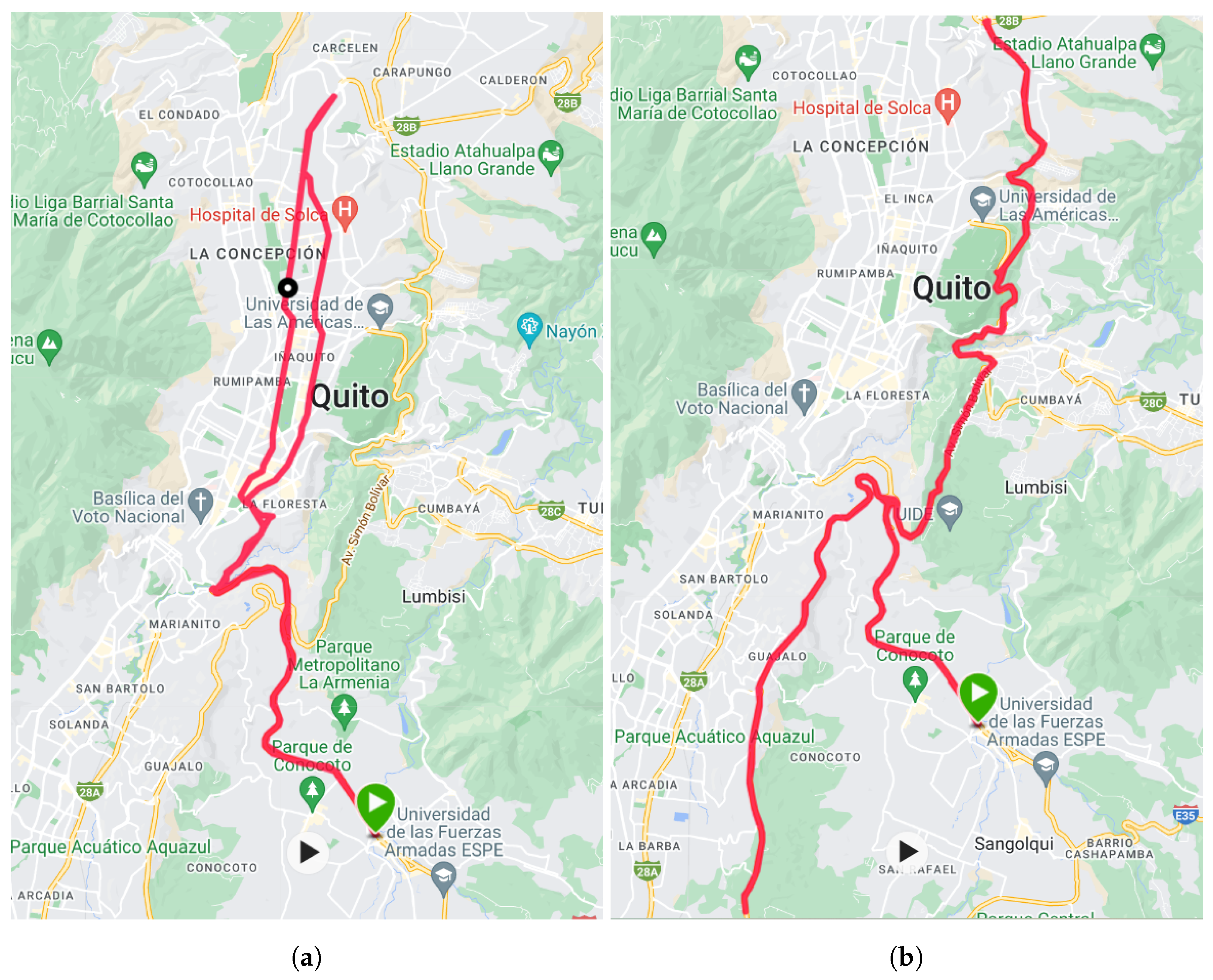
3.5. Routes and Timetables

We considered roads with high traffic accident rates and roads with heavy traffic in the urban area of Quito, Ecuador. In this way, the experiment considered Simón Bolívar avenue as a high-rate accident road, General Rumiñahui highway, Velasco Ibarra, 6 de Diciembre, Galo Plaza Lasso, and Amazonas avenues as high-traffic roads. The experiment considered the two routes described below. Figure 2 presents the routes on the maps.

• Route 1 is 59 km long that begins on the General Rumiñahui highway, crosses Velasco Ibarra, Ladrón de Guevara, Patria, 6 de Diciembre, and Galo Plaza Lasso avenues, returns by Galo Plaza Lasso, Amazonas, Patria, and Velasco Ibarra avenues, and finishes on the General Rumiñahui highway.
• Route 2 is 96 km long that begins on the General Rumiñahui highway, continues with the Simón Bolívar avenue in the south-north direction, returns by the Simón Bolívar in the north-south direction, and finishes on the General Rumiñahui.

3.6. Control Points

We referenced several control points along the two routes geographically. Both routes were divided into segments with a start and end point and many control points for each segment [21]. These points helped us calculate the number of traffic accidents around them and determine the design speeds along the route. Thus, Route 1 counts 90 segments and 557 control points, and Route 2 counts 191 and 615 control points.

Table 6. Sample of control points for Routes 1 and 2.

Route	Road ID	Segment	Starting Point			End Point
			ID	Latitude	Longitude	ID	Latitude	Longitude
1	AGR	S01	P001	−0.29755	−78.46091	P008	−0.29065	−78.46514
	AGR	S21	P066	−0.2267	−78.48815	P069	−0.2271	−78.49302
	DMQ	S41	P252	−0.10668	−78.47647	P256	−0.10049	−78.47192
	AVI	S61	P431	−0.21767	−78.49135	P434	−0.21874	−78.49304
	AGR	S89	P544	−0.28173	−78.47117	P550	−0.28893	−78.46642
2	AGR	S001	P001	−0.29755	−78.46091	P008	−0.29065	−78.46514
	ASB	S041	P121	−0.18184	−78.45117	P122	−0.18123	−78.45135
	ASB	S081	P223	−0.16034	−78.44692	P226	−0.16671	−78.44792
	ASB	S121	P348	−0.26910	−78.50768	P350	−0.2717	−78.50844
	ASB	S173	P538	−0.23428	−78.49155	P539	−0.23394	−78.49249

presents a sample of control points for Routes 1 and 2.

Table A2. Extended sample of control points for Route 1.

Road ID	Segment	Starting Point			End Point
		ID	Latitude	Longitude	ID	Latitude	Longitude
AGR	S01	P001	−0.29755	−78.46091	P008	−0.29065	−78.46514
AGR	S03	P016	−0.28166	−78.47105	P018	−0.27999	−78.47296
AGR	S05	P022	−0.27837	−78.48127	P024	−0.27687	−78.48597
AGR	S07	P028	−0.27093	−78.48937	P030	−0.26995	−78.48797
AGR	S09	P034	−0.26585	−78.48679	P035	−0.26472	−78.4874
AGR	S11	P039	−0.25961	−78.48721	P041	−0.2572	−78.48505
AGR	S13	P045	−0.25224	−78.48292	P047	−0.24996	−78.48282
AGR	S15	P050	−0.24518	−78.48492	P052	−0.24281	−78.48542
AGR	S17	P055	−0.23902	−78.48485	P057	−0.23649	−78.48426
AGR	S19	P061	−0.23038	−78.48455	P062	−0.22925	−78.485
AGR	S21	P066	−0.2267	−78.48815	P069	−0.2271	−78.49302
AGR	S23	P073	−0.22974	−78.4974	P076	−0.23261	−78.5013
AVI	S25	P079	−0.23224	−78.50294	P085	−0.22943	−78.50077
AVI	S27	P096	−0.22479	−78.49702	P104	−0.22108	−78.4952
AVI	S29	P112	−0.21797	−78.49151	P121	−0.21309	−78.48891
DMQ	S31	P125	−0.21252	−78.48894	P136	−0.21047	−78.49363
DMQ	S33	P142	−0.20853	−78.4953	P155	−0.20255	−78.48677
DMQ	S35	P167	−0.19188	−78.48108	P184	−0.17915	−78.47825
DMQ	S37	P203	−0.16393	−78.47518	P212	−0.15587	−78.47696
DMQ	S39	P231	−0.13687	−78.47347	P246	−0.12179	−78.47898
DMQ	S41	P252	−0.10668	−78.47647	P256	−0.10049	−78.47192
DMQ	S43	P278	−0.12921	−78.48137	P287	−0.13844	−78.48264
DMQ	S45	P304	−0.15324	−78.48467	P309	−0.15792	−78.48439
DMQ	S47	P335	−0.16911	−78.48446	P343	−0.17452	−78.48541
DMQ	S49	P356	−0.18705	−78.4876	P363	−0.19128	−78.48837
DMQ	S51	P370	−0.19677	−78.4896	P375	−0.19962	−78.49078
DMQ	S53	P385	−0.20248	−78.49399	P392	−0.20498	−78.49547
DMQ	S55	P400	−0.20767	−78.49708	P403	−0.20847	−78.49612
DMQ	S57	P408	−0.20969	−78.49451	P413	−0.21136	−78.49354
DMQ	S59	P419	−0.21286	−78.49219	P426	−0.21485	−78.49106
AVI	S61	P431	−0.21767	−78.49135	P434	−0.21874	−78.49304
AVI	S63	P441	−0.22278	−78.4959	P447	−0.22604	−78.49801
AVI	S65	P452	−0.22743	−78.50016	P456	−0.22973	−78.50097
AGR	S67	P461	−0.23214	−78.50301	P465	−0.23355	−78.50293
AGR	S69	P470	−0.22983	−78.49735	P473	−0.22788	−78.49466
AGR	S71	P478	−0.22679	−78.48822	P480	−0.22803	−78.48646
AGR	S73	P484	−0.23039	−78.48466	P487	−0.23437	−78.48442
AGR	S75	P491	−0.23897	−78.48499	P493	−0.24082	−78.48563
AGR	S77	P498	−0.24522	−78.48505	P501	−0.24799	−78.48381
AGR	S79	P506	−0.25222	−78.48304	P509	−0.25514	−78.4842
AGR	S81	P514	−0.25952	−78.4873	P517	−0.26273	−78.48834
AGR	S83	P521	−0.26591	−78.48694	P524	−0.26888	−78.48705
AGR	S85	P528	−0.27084	−78.48943	P531	−0.27565	−78.48944
AGR	S87	P536	−0.27851	−78.48131	P539	−0.27954	−78.47542
AGR	S89	P544	−0.28173	−78.47117	P550	−0.28893	−78.46642

AGR—General Rumiñahui Highway. DMQ—Metropolitan District of Quito. AVI—Velasco Ibarra Avenue..

and

Table A3. Extended sample of control points for Route 2.

Road ID	Segment	Starting Point			End Point
		ID	Latitude	Longitude	ID	Latitude	Longitude
AGR	S001	P001	−0.29755	−78.46091	P008	−0.29065	−78.46514
AGR	S003	P016	−0.28166	−78.47105	P018	−0.27999	−78.47296
AGR	S005	P022	−0.27837	−78.48127	P024	−0.27687	−78.48597
AGR	S007	P028	−0.27093	−78.48937	P030	−0.26995	−78.48797
AGR	S009	P034	−0.26585	−78.48679	P035	−0.26472	−78.4874
AGR	S011	P039	−0.25961	−78.48721	P041	−0.2572	−78.48505
AGR	S013	P045	−0.25224	−78.48292	P047	−0.24996	−78.48282
AGR	S015	P050	−0.24518	−78.48492	P052	−0.24281	−78.48542
ASB	S017	P055	−0.23945	−78.48496	P059	−0.24315	−78.48256
ASB	S019	P063	−0.24625	−78.47657	P065	−0.24202	−78.47433
ASB	S021	P069	−0.23615	−78.47298	P071	−0.2347	−78.47095
ASB	S023	P074	−0.23041	−78.46985	P075	−0.22942	−78.46914
ASB	S025	P081	−0.21675	−78.46567	P082	−0.21539	−78.46449
ASB	S027	P085	−0.21146	−78.46253	P087	−0.20665	−78.46084
ASB	S029	P090	−0.20322	−78.45855	P092	−0.20021	−78.45669
ASB	S031	P095	−0.19828	−78.46070	P096	−0.19839	−78.46164
ASB	S033	P099	−0.19860	−78.46491	P100	−0.19808	−78.46644
ASB	S035	P104	−0.19546	−78.46405	P106	−0.19399	−78.46052
ASB	S037	P109	−0.19199	−78.45866	P110	−0.19187	−78.45795
ASB	S039	P116	−0.18772	−78.45412	P118	−0.18511	−78.45273
ASB	S041	P121	−0.18184	−78.45117	P122	−0.18123	−78.45135
ASB	S043	P126	−0.18105	−78.45391	P127	−0.18037	−78.45582
ASB	S045	P132	−0.17279	−78.45193	P134	−0.16996	−78.44987
ASB	S047	P137	−0.16384	−78.44792	P139	−0.16106	−78.44722
ASB	S049	P143	−0.15681	−78.44634	P145	−0.15338	−78.44721
ASB	S051	P148	−0.15191	−78.45150	P149	−0.15133	−78.45193
ASB	S053	P152	−0.14980	−78.45068	P153	−0.14874	−78.44897
ASB	S055	P156	−0.14762	−78.44748	P158	−0.14553	−78.44521
ASB	S057	P162	−0.14044	−78.44466	P165	−0.13719	−78.44722
ASB	S059	P169	−0.12963	−78.44828	P170	−0.12791	−78.44828
ASB	S061	P173	−0.11840	−78.45088	P176	−0.11325	−78.45675
ASB	S063	P179	−0.11025	−78.45799	P181	−0.10953	−78.45877
ASB	S065	P184	−0.11193	−78.45749	P185	−0.11529	−78.45485
ASB	S067	P188	−0.11850	−78.45096	P189	−0.1214	−78.44807
ASB	S069	P192	−0.12649	−78.44817	P194	−0.12866	−78.44853
ASB	S071	P197	−0.13510	−78.44764	P199	−0.13834	−78.44709
ASB	S073	P202	−0.14055	−78.44478	P204	−0.14354	−78.44382
ASB	S075	P209	−0.14750	−78.44751	P210	−0.14772	−78.44819
ASB	S077	P215	−0.15078	−78.45246	P216	−0.15157	−78.45197
ASB	S079	P219	−0.15268	−78.44880	P220	−0.15434	−78.44667
ASB	S081	P223	−0.16034	−78.44692	P226	−0.16671	−78.44792
ASB	S083	P232	−0.17604	−78.45459	P233	−0.17624	−78.45568
ASB	S085	P236	−0.17890	−78.45535	P238	−0.18152	−78.45518
ASB	S087	P241	−0.18048	−78.45218	P243	−0.18321	−78.45104
ASB	S089	P246	−0.18528	−78.45344	P247	−0.18683	−78.45409
ASB	S091	P252	−0.19196	−78.45678	P256	−0.19365	−78.46142
ASB	S093	P262	−0.19875	−78.46491	P268	−0.20245	−78.45792
ASB	S095	P274	−0.20831	−78.46164	P276	−0.2107	−78.46236
ASB	S097	P279	−0.21265	−78.46373	P280	−0.21386	−78.46407
ASB	S099	P283	−0.21886	−78.46671	P285	−0.22464	−78.4689
ASB	S101	P288	−0.23032	−78.46996	P289	−0.23107	−78.47046
ASB	S103	P294	−0.23612	−78.47313	P301	−0.24518	−78.47624
ASB	S105	P306	−0.24405	−78.48218	P307	−0.2426	−78.48259
ASB	S107	P315	−0.23294	−78.48880	P316	−0.2324	−78.48933
ASB	S109	P319	−0.23372	−78.49296	P320	−0.23427	−78.49205
ASB	S111	P325	−0.23918	−78.49250	P326	−0.23962	−78.49314
ASB	S113	P329	−0.24229	−78.49592	P331	−0.24285	−78.49992
ASB	S115	P334	−0.24686	−78.50143	P336	−0.24954	−78.50271
ASB	S117	P340	−0.25545	−78.50350	P341	−0.25677	−78.50286
ASB	S119	P344	−0.26252	−78.50514	P345	−0.26535	−78.50739
ASB	S121	P348	−0.26910	−78.50768	P350	−0.2717	−78.50844
ASB	S123	P353	−0.27629	−78.51247	P357	−0.28423	−78.51812
ASB	S125	P360	−0.28624	−78.51907	P362	−0.28904	−78.51979
ASB	S127	P369	−0.30256	−78.52161	P377	−0.31294	−78.52237
ASB	S129	P383	−0.32332	−78.52019	P384	−0.3278	−78.5191
ASB	S131	P388	−0.33475	−78.52013	P390	−0.33721	−78.52059
ASB	S133	P393	−0.34284	−78.52297	P396	−0.34739	−78.52354
ASB	S135	P399	−0.34887	−78.52331	P403	−0.35486	−78.5252
ASB	S137	P409	−0.35741	−78.53344	P410	−0.35913	−78.53468
ASB	S139	P414	−0.36507	−78.52912	P415	−0.36585	−78.52861
ASB	S141	P428	−0.38228	−78.53171	P432	−0.38417	−78.5321
ASB	S143	P437	−0.37681	−78.53043	P444	−0.36893	−78.52879
ASB	S145	P449	−0.36497	−78.52902	P452	−0.36132	−78.53296
ASB	S147	P456	−0.35756	−78.53338	P457	−0.35719	−78.53073
ASB	S148	P458	−0.35664	−78.52849	P459	−0.35615	−78.52749
ASB	S149	P460	−0.35530	−78.52579	P463	−0.35066	−78.52291
ASB	S151	P466	−0.34804	−78.52329	P468	−0.3455	−78.52364
ASB	S153	P473	−0.33478	−78.51997	P475	−0.33226	−78.51952
ASB	S155	P480	−0.32329	−78.52007	P483	−0.31841	−78.52146
ASB	S157	P491	−0.30257	−78.52146	P496	−0.29606	−78.52032
ASB	S159	P499	−0.29047	−78.51954	P501	−0.28754	−78.51955
ASB	S161	P504	−0.28501	−78.51836	P509	−0.27542	−78.51148
ASB	S163	P512	−0.26912	−78.50753	P513	−0.26859	−78.50741
ASB	S165	P516	−0.26259	−78.50504	P518	−0.25822	−78.50242
ASB	S167	P521	−0.25015	−78.50296	P522	−0.24903	−78.50217
ASB	S169	P525	−0.24465	−78.50078	P528	−0.24266	−78.4972
ASB	S171	P531	−0.24073	−78.49421	P532	−0.23996	−78.4934
ASB	S173	P538	−0.23428	−78.49155	P539	−0.23394	−78.49249
ASB	S175	P542	−0.23151	−78.49158	P543	−0.2319	−78.49016
AGR	S177	P552	−0.24168	−78.4858	P555	−0.24447	−78.48527
AGR	S179	P560	−0.24873	−78.48341	P563	−0.25167	−78.4829
AGR	S181	P568	−0.25581	−78.48447	P571	−0.25897	−78.48675
AGR	S183	P576	−0.26355	−78.48809	P578	−0.26529	−78.48724
AGR	S185	P583	−0.26953	−78.4876	P585	−0.27054	−78.48902
AGR	S187	P590	−0.27625	−78.48834	P593	−0.27811	−78.48255
AGR	S189	P598	−0.27964	−78.47458	P601	−0.28115	−78.4716
AGR	S191	P609	−0.29028	−78.46552	P615	−0.29759	−78.46097

ASB—Simón Bolívar Avenue.

in Appendix A present the whole lists for Routes 1 and 2, respectively. Figure 3 presents a sample of the control points on the map.

4. Results

The POLIDriving dataset contains data from seven data acquisition sessions. Five drivers and four vehicles participated and were used in the sessions. Additionally, we generated two extra sessions with synthetic data based on real data. POLIDriving contains around 18 h of driving data and 32 attributes from five heterogeneous sources. All the raw and processed data files are stored in a public GitHub repository [22].

Table 7. Sample of data file.

Time	Speed	rpm	Acceleration	Throttle Position	Engine Temperature	System Voltage	Distance Travelled	Engine Load Value
15:33:15	65	2306	−0.7279	26.2745	97	12.6	18.4204	17.6470
15:33:16	62	2246	−0.7488	32.9411	97	12.6	18.4346	47.0588
15:33:17	61	2217	−0.2281	36.4705	97	12.6	18.4452	49.4117
15:33:18	61	2201	0.0	40.0	96	12.6	18.4673	65.0980
15:33:19	61	2225	0.0	72.5490	96	12.6	18.4788	76.8627
15:33:20	62	2258	0.0	81.9607	96	12.7	18.4992	80.7843
Time	Altitude	id Vehicle	Latitude	Longitude	id Driver	Heart Rate	Body Temperature	Current Weather
15:33:15	2586.61	4	−0.195041	−78.463115	4	64	29	Clouds and sun
15:33:16	2587.17	4	−0.194989	−78.462963	4	64	29	Clouds and sun
15:33:17	2587.40	4	−0.19493	−78.462816	4	64	29	Clouds and sun
15:33:18	2588.94	4	−0.194862	−78.462684	4	64	29	Clouds and sun
15:33:19	2589.78	4	−0.194783	−78.46256	4	64	29	Clouds and sun
15:33:20	2590.04	4	−0.194683	−78.462441	4	64	29	Clouds and sun
Time	Has Precipitation	Is Day Time	Temperature	Wind Speed	Wind Direction	Relative Humidity	Visibility	uv Index
15:33:15	FALSE	TRUE	19.5	14.5	0	62	8	2
15:33:16	FALSE	TRUE	19.5	14.5	0	62	8	2
15:33:17	FALSE	TRUE	19.5	14.5	0	62	8	2
15:33:18	FALSE	TRUE	19.5	14.5	0	62	8	2
15:33:19	FALSE	TRUE	19.5	14.5	0	62	8	2
15:33:20	FALSE	TRUE	19.5	14.5	0	62	8	2
Time	Cloud Cover	Ceiling	Pressure	Precipitation	Accidents Onsite	Design Speed	Accidents Time
15:33:15	74	3139	1019.6	2.4	8	50	3
15:33:16	74	3139	1019.6	2.4	7	70	3
15:33:17	74	3139	1019.6	2.4	8	70	3
15:33:18	74	3139	1019.6	2.4	8	70	3
15:33:19	74	3139	1019.6	2.4	8	70	3
15:33:20	74	3139	1019.6	2.4	9	70	3

presents a sample of the processed data file for the Alonso user for Route 1.

To test POLIDriving, we selected the traffic accident prediction research area, specifically predicting risk levels by identifying risky driving patterns. In that way, we built two learning models, one based on neural networks and the other on decision trees. First of all, we performed data integration to join data from the Accuweather web service and the traffic accident and road geometric characteristics databases. Then, we performed data cleaning and feature selection over POLIDriving. It was reduced to 14 attributes out of 32 available ones. Low variance filters and correlation and mutual information matrices were used to select the most relevant attributes. Figure 4 presents the correlation matrix before and after the feature selection.

Once preprocessing was performed, we manually labeled a very small portion of the observations. Then, we used semi-supervised techniques and a voting ensemble to label the rest. For manual labeling, we identified threshold values for the attributes and established ranges and their penalties.

Table 8. Sample of threshold values and ranges for manual data labeling.

#	Attribute	Item	ID	Value Range	Penalty
1	rpm	very high	-	[5001–8000]	3
2	engine temperature	overheating	-	[105–200]	2
3	heart rate	tachycardia severe	-	[121–180]	4
4	weather types	rain	18	-	4
5	visibility	bad	-	[0.0–0.0]	4
6	precipitation	violent	-	[50.1–100.0]	4
7	accidents on site	very high	-	[133–300]	4
8	design speed	very serious	-	[41–100]	4
9	accidents time	high	-	[10–100]	3

presents a sample of threshold values and ranges used by experts for manual data labeling, and

Table A1. Threshold values and ranges for manual data labeling.

#	Attribute	Item	ID	Value Range	Penalty
1	rpm	low		[0–1500]	1
2		normal		[1501–3000]	0
3		high		[3001–5000]	2
4		very high		[5001–8000]	3
5	engine temperature	low		[0–82]	1
6		normal		[83–94]	0
7		high		[95–104]	1
8		overheating		[105–200]	2
9	heart rate	bradicardia		[0–59]	2
10		sinus zona a		[60–80]	1
11		sinus zona b		[81–100]	2
12		tachycardia slight		[101–120]	3
13		tachycardia severe		[121–180]	4
14	weather types	sunny	1		1
15		mostly sunny	2		1
16		partly sunny	3		1
17		hazy sunshine	5		1
18		mostly cloudy	6		2
19		cloudy	7		2
20		clouds and sun	9		2
21		partly cloudy	35		3
22		fog	11		3
23		rain	18		4
24	visibility	bad		[0.0–0.0]	4
25		poor		[0.1–2.4]	3
26		moderate		[2.5–10.0]	2
27		good		[10.1–50.0]	1
28		excellent		[50.1–100.0]	0
29	precipitation	none		[0.0–0.0]	0
30		light		[0.1–2.4]	1
31		moderate		[2.5–10.0]	2
32		heavy		[10.1–50.0]	3
33		violent		[50.1–100.0]	4
34	accidents on site	none		[0–0]	0
35		low		[1–8]	1
36		moderate		[9–30]	2
37		high		[31–132]	3
38		very high		[133–300]	4
39	design speed	normal		[0–0]	0
40		slight		[1–10]	1
41		moderate		[11–20]	2
42		serious		[21–40]	3
43		very serious		[41–100]	4
44	accidents time	none		[0–0]	0
45		low		[1–2]	1
46		moderate		[3–9]	2
47		high		[10–100]	3

in Appendix A presents the whole list of threshold values and ranges. We determined the risk level among low, medium, high, and very high depending on the number of penalties. Since few observations were labeled with high-risk levels, extra observations with synthetic data presenting risky driving patterns were added. It permitted labeling 8.5% of the total observations (23.152). From the total of labeled observations (1.980), we considered 75% (1.485) for training and 25% (495) for testing. Unlabeled observations (21.172) were labeled using a voting ensemble with labels generated by semi-supervised learning methods such as label propagation, label spreading, and self-training based on Multilayer Perceptron, Random Forest, and Gradient Boosting Machine.

Table 9. Evaluation of data labeling.

#	Method	Hyperparameters	Accuracy
1	Label propagation (LP)	alpha = 0.2, gamma = 0.1, kernel = knn, number_neighbors = 10, and maximum_iterations = 5000	0.71
2	Label spreading (LS)	gamma = 0.1, kernel = knn, number_neighbors = 15, and maximum_iterations = 5000	0.75
3	Self training (SVM)	kernel = rbf, probability = True, and gamma = 0.1	0.62
4	Self training (MLP)	activation_function = relu, hidden_layers = 3, neurons_per_layer = 30, learning_rate = constant, maximum_iterations = 5000, and solver = adam	0.84
5	Self training (RF)	number_estimators = 50, maximum_depth = None, minimum_samples_leaf = 1, maximum_features = sqrt, and minimum_samples_split = 2	0.83
6	Self training (GBM)	learning_rate = 0.8, maximum_depth = 30, number_estimators = 100, minimum_samples_leaf = 1, maximum_features = None, and minimum_samples_split = 2	0.82
7	Ensemble	estimators = [LP, LS, MLP, RF, GBM] and voting = hard	0.82

presents the results of the labeling data.

Despite the strategies applied to add observations, the dataset was still unbalanced, so we applied the oversampling technique known as SMOTE [23]. It helped to balance all the minority classes with the majority class. Thus, the dataset reached values of 12.839 for every risk level. Considering the most common algorithms used in prediction models for traffic accident prevention proposed by [2], we built two models; the first used a Gradient Boosting Machine (GBM) with 100 estimators, a learning rate of 0.1, a maximum depth of 3, and relu as the activation function, and the second one used a Multilayer Perceptron (MLP) with three hidden layers, 100 neurons for each layer, and the hyperbolic tangent as the activation function.

Table 10. Configuration of the learning models.

#	Algorithm	Hyperparameters
1	Gradient Boosting Machine (GBM)	learning_rate = 0.8, loss_function = log_loss, maximum_depth = 30, maximum_features = sqrt, minimum_samples_split = 0.5, and number_estimators = 100
2	Multilayer Perceptron (MLP)	activation_function = tanh, hidden_layers = 3, neurons_per_layer = 100, learning_rate = adaptive, maximum_iterations = 1000, and solver = lbfgs

presents the configurations for the learning models. Both models were trained and evaluated using cross-validation with ten folds.

Table 11. Evaluation of the learning models.

#	Algorithm	Folds	Results	Avg. Accuracy
1	GBM	10	[0.95713157, 0.95673647, 0.9589014, 0.95238095, 0.95751828, 0.9608773, 0.95573997, 0.95593756, 0.95692551, 0.95732069]	0.956
2	MLP	10	[0.98656657, 0.98636902, 0.98794705, 0.9832049, 0.98656392, 0.98755187, 0.9869591, 0.98676151, 0.9869591, 0.98794705]	0.986

presents the evaluation of the learning models.

Finally,

Table 12. Sample of observations and their predicting classes.

Hour	Speed	rpm	Accel.	Throttle Pos.	Eng. Temp.	Eng. Load Value	Heart Rate	Curr. Weather	Visib.	Precip.	Acdnt. on Site	Design Speed	Acdnt. That Time	Risk Level
15	114	3251	−0.64	17.6	94	23.5	100	rain	3.2	8	10	90	1	very high
15	26	3934	1.48	74.1	96	22.7	102	rain	3.2	8	105	90	6	very high
15	26	3540	1.8	76.1	97	94.5	102	rain	3.2	8	105	90	6	very high
15 *	81	2950	0.22	60	94	58	118	rain	3.2	8	12	80	3	very high
16	44	2099	0.41	16.1	92	22	101	cloudy	8	24	248	80	15	very high
16	129	3694	0.14	31.8	91	87.5	96	cloudy	8	8	4	80	0	high
19	102	3895	0	49	94	91	84	cloudy	6.4	4.8	28	70	1	high
15	78	2873	−0.27	34.1	94	85.9	118	rain	3.2	8	10	80	3	high
16	61	2223	−0.13	30.6	94	91.8	106	cloudy	8	24	37	60	1	high
15	76	2184	0.1	20.4	94	57.3	94	rain	3.2	0	254	90	10	high
16	126	3573	0.29	65.1	94	86.7	94	cloudy	8	8	7	90	0	medium
19	58	4413	0.46	40	91	81.2	84	cloudy	6.4	0	82	90	3	medium
15	84	2402	0.26	16.5	91	21.6	113	cloudy	8	0	5	60	0	medium
16	78	2820	0	76.9	94	90.2	104	cloudy	8	24	11	70	0	medium
16	84	2410	0.25	43.1	95	26.3	67	mostly cloudy	16.1	1.3	253	90	14	medium
20	122	3466	0.49	28.6	92	71	89	cloudy	8	0	38	90	1	low
20	54	4177	0.47	40.4	93	91.4	85	cloudy	8	0	2	70	0	low
15	98	3832	0.56	78.8	92	63.9	104	cloudy	8	0	15	90	1	low
16	66	2316	0.34	18.8	91	34.5	98	cloudy	8	24	5	90	0	low
16	74	2680	0.54	82	95	80	74	hazy sunshine	16.1	0	246	90	16	low

* See the explanation of this observation in Section 4.

presents a random sample of observations and their predicting classes. The observation marked with (*15) can be interpreted as follows. That observation received the risk level ’very high’ because the driver speeded at 81 km/h, exceeding the designated speed of 80 km/h. Her/his vehicle worked in normal conditions, with an engine temperature of 94 °C and at 2950 rpm, low of normal range. However, the driver presented a slight tachycardia (101 bpm), probably due to anxiety or stress, while driving in adverse rain conditions with low visibility (3.2 km) and precipitation of 8 mm. Finally, the driver crossed through a road with a moderate traffic accident rate of 12 and a moderate traffic accident rate at a specific hour of 3.

5. Discussion

Although several driving datasets are available, most target the autonomous driving area, and the rest are very limited in terms of the reduced number of data sources and attributes, not to mention that the best ones are not free public access. This fact motivated the creation of a new dataset. As mentioned, this work aimed to create a driving dataset that targets the driving behavior area and correlates and integrates information from heterogeneous sources. Thus, we created a public driving dataset, which we named POLIDriving.

In comparison with related datasets in which the vehicles used in the acquisition sessions were equipped with high-resolution cameras, LIDAR radars, long-rage radars, OBD-II scanners, GNSS receivers, and IMU devices, in our dataset, the vehicles were equipped with an acquisition module which consists of a GNSS receiver, an OBD-II scanner, and a smartphone. This option was adopted because POLIDriving is intended to focus on driving behavior, not autonomous driving applications. Finally, although adding advanced equipment to vehicles to improve the dataset sounds tempting, a dataset that includes information from fully equipped vehicles is not viable because of resource limitations and mainly because such a dataset is beyond the aim of this study.

In numbers, POLIDriving includes information from five heterogeneous data sources in contrast to two data sources of the related datasets. Similarly, POLIDriving can have more or less the same number of attributes (around 40) as the related datasets; however, its attributes are not from only one or two sources. Instead, POLIDriving has 13 attributes related to vehicle data, three to driver’s data, 13 to weather data, two to traffic accidents, and one to road geometric characteristics.

As mentioned above, POLIDriving focuses on driving behavior so that it could be used, for instance, in applications related to identifying risky driving behaviors in drivers. Therefore, having information from different drivers is desirable in those applications. In accordance with this, we recruited many drivers to participate in the acquisition sessions. In comparison with the rest of the related datasets, POLIDriving used more drivers, five to be exact, of different ages, genders, and driving experience. Finally, we decided that every driver should use the vehicle that drives daily to avoid unusual driving behaviors.

Something to consider is how driving behavior influences the risk of suffering a traffic accident, as well as, how prone a driver with aggressive driving behavior is to accidents. According to the United Nations Economic Commission for Europe (UNECE), typical aggressive driving behavior includes speeding, not respecting traffic signals, or changing lanes inappropriately. Therefore, looking for more evidence confirming that aggressive driving behavior is closely related to a high probability of accidents is unnecessary. In this way, we added synthetic data for an unreal driver (furious) based on a real drive to POLIDriving. This driver is speeding, driving at very high rpm, and experiencing anxiety and stress, reflected by a very high heart rate.

Once POLIDriving was released, it was tested in a model to predict risk levels of suffering traffic accidents. We tried combining semi-supervised and ensemble learning techniques for data labeling. It allowed us to label 91.5% of observations using only 8.5% of labeled observations with an accuracy of 82.0%. This result is a great achievement, considering the accuracies of 71.0% and 75.0% obtained by the label propagation and spreading methods. The other great achievement was the accuracies of 95.6% and 98.6% obtained by the supervised learning models. It was accomplished by performing a cross-validation technique for tuning hyperparameters of the learning model. These achievements and the result of an audit method applied to a representative amount of observations ratified the good quality of the POLIDriving dataset.

Since POLIDriving uses different data sources, potential biases related to them must be analyzed and resolved. Biases concerning the weather service include the insufficient spatial resolution of the weather model and the updating frequency of only one observation per hour. In other words, the current conditions of a location can be better fit using the conditions of other nearby locations. Similarly, the conditions can change rapidly in very changing climates, so the updating frequency (1 sample/hour) must be higher to avoid having erroneous current conditions. A possible solution could be installing a portable weather station in the vehicle.

Future work should integrate information from other data sources, such as traffic flow or traffic events, into POLIDriving. For instance, as part of the traffic flow, attributes such as the number of vehicles and occupancy, and as part of the traffic events, attributes such as closures, broken vehicles, congestion, and blocked lanes [2]. Furthermore, POLIDriving could be improved for future acquisition sessions by including more women and senior adults as drivers, passenger transport (taxis), and emergency vehicles, as well as by designing new routes that include roads in rural areas and highways. Finally, and based on these studies [24,25], POLIDriving could be improved by installing a front-facing camera to identify gestures or grimaces associated with aggressive behavior or using already available attributes to recognize aggressive driving styles such as aggressive, distracted, or drunk driving.

6. Conclusions

We obtained a public driving dataset that targets driving behavior, specifically road traffic safety, and stands out for its heterogeneity. Our non-expensive and easy installation acquisition agent allowed us to use different types of vehicles in the acquisition sessions. Thus, we could engage more drivers and their vehicles to avoid unusual driving behaviors. The lack of driving datasets with the heterogeneity feature motivated us to create a dataset with as many different sources as possible. Thus, we also integrated data from external databases and web services related to traffic accidents, road geometric characteristics, and weather conditions.

Once built, the POLIDriving dataset allowed us to design and test learning models for road traffic safety. We tested the built dataset with our designed model to predict risk levels of suffering an accident. As you know, the performance of a learning model depends largely on the quality of the dataset used to train and test the model. The results confirmed, therefore, the good quality of POLIDriving, which also made us think that other authors will use our dataset in their applications. Undoubtedly, the POLIDriving dataset will greatly contribute to research on road traffic safety and will be a great asset to the community.

However, our dataset is not without its limitations, notably in the representation of gender and age demographics among participants and the variety of driving conditions tested. Future enhancements will address these gaps by incorporating a more balanced participant pool and designing studies that simultaneously analyze driving behaviors across diverse routes.

We strongly advocate for the continued expansion and refinement of POLIDriving. The dataset can offer even deeper insights into driving behaviors and traffic safety by including broader demographic and situational diversity. We invite the research community to explore POLIDriving for their projects, believing that collaborative efforts will propel forward our shared goal of improving road safety.

References

- World Health Organization. WHO Global Status Report on Road Safety 2023; WHO: Geneva, Switzerland, 2023. [Google Scholar]
- Marcillo, P.; Valdivieso Caraguay, Á.L.; Hernández-Álvarez, M. A Systematic Literature Review of Learning-Based Traffic Accident Prediction Models Based on Heterogeneous Sources. Appl. Sci. 2022, 12, 4529. [Google Scholar] [CrossRef]
- Geyer, J.; Kassahun, Y.; Mahmudi, M.; Ricou, X.; Durgesh, R.; Chung, A.S.; Hauswald, L.; Pham, V.H.; Mühlegg, M.; Dorn, S.; et al. A2d2: Audi autonomous driving dataset. arXiv 2020, arXiv:2004.06320. [Google Scholar]
- Geiger, A.; Lenz, P.; Stiller, C.; Urtasun, R. Vision meets robotics: The kitti dataset. Int. J. Robot. Res. 2013, 32, 1231–1237. [Google Scholar] [CrossRef]
- Yu, F.; Chen, H.; Wang, X.; Xian, W.; Chen, Y.; Liu, F.; Madhavan, V.; Darrell, T. Bdd100k: A diverse driving dataset for heterogeneous multitask learning. In Proceedings of the IEEE/CVF Conference on Computer Vision and Pattern Recognition, Seattle, WA, USA, 14–19 June 2020; pp. 2636–2645. [Google Scholar]
- Huang, X.; Wang, P.; Cheng, X.; Zhou, D.; Geng, Q.; Yang, R. The apolloscape open dataset for autonomous driving and its application. IEEE Trans. Pattern Anal. Mach. Intell. 2019, 42, 2702–2719. [Google Scholar] [CrossRef] [PubMed]
- Santana, E.; Hotz, G. Learning a driving simulator. arXiv 2016, arXiv:1608.01230. [Google Scholar]
- Schafer, H.; Santana, E.; Haden, A.; Biasini, R. A commute in data: The comma2k19 dataset. arXiv 2018, arXiv:1812.05752. [Google Scholar]
- Izquierdo, R.; Quintanar, A.; Parra, I.; Fernández-Llorca, D.; Sotelo, M. The prevention dataset: A novel benchmark for prediction of vehicles intentions. In Proceedings of the 2019 IEEE Intelligent Transportation Systems Conference (ITSC), Auckland, New Zealand, 27–30 October 2019; IEEE: Piscataway, NJ, USA, 2019; pp. 3114–3121. [Google Scholar]
- Weber, M. Automotive OBD-II Dataset. 2023. Available online: https://radar.kit.edu/radar/en/dataset/bCtGxdTklQlfQcAq (accessed on 27 April 2024).
- Veepeak. OBDCheck BLE+. Available online: https://www.veepeak.com/product/obdcheck-ble-plus/ (accessed on 27 April 2024).
- Garmin. Vivosmart 5. Available online: https://www.garmin.com/en-US/p/782585 (accessed on 27 April 2024).
- ISO 11898-1:2015; Road Vehicles—Controller Area Network (CAN). Part 1: Data Link Layer and Physical Signalling. International Organization for Standardization: Geneva, Switzerland, 2015. Available online: https://www.iso.org/standard/63648.html (accessed on 27 April 2024).
- ISO 14230-1:2012; Road Vehicles—Diagnostic Communication over K-Line (DoK-Line). International Organization for Standardization: Geneva, Switzerland, 2012. Available online: https://www.iso.org/standard/55591.html (accessed on 27 April 2024).
- ISO 9141-2:1994; Road Vehicles—Diagnostic Systems. Part 2: CARB Requirements for Interchange of Digital Information. International Organization for Standardization: Geneva, Switzerland, 1994. Available online: https://www.iso.org/standard/16738.html (accessed on 27 April 2024).
- J1850_202212; Class B Data Communications Network Interface (STABILIZED Dec 2022). SAE International: Warrendale, PA, USA, 2022. Available online: https://www.sae.org/standards/content/j1850_202212/ (accessed on 27 April 2024).
- Accuweather. Accuweather. Available online: https://www.accuweather.com/ (accessed on 27 April 2024).
- Transit National Agency (ANT). National Accident Rate Viewer. Available online: https://www.ant.gob.ec/visor-de-siniestralidad-estadisticas/ (accessed on 27 April 2024).
- Yan, Y.; Zhang, Y.; Yang, X.; Hu, J.; Tang, J.; Guo, Z. Crash prediction based on random effect negative binomial model considering data heterogeneity. Phys. A Stat. Mech. Its Appl. 2020, 547, 123858. [Google Scholar] [CrossRef]
- Bao, J.; Liu, P.; Ukkusuri, S.V. A spatiotemporal deep learning approach for citywide short-term crash risk prediction with multi-source data. Accid. Anal. Prev. 2019, 122, 239–254. [Google Scholar] [CrossRef] [PubMed]
- Heredia Silva, C.A. Desarrollo de potenciales aplicaciones móviles aplicables al estudio de velocidades seguras en vías. Caso de estudio: Avenida Simón Bolívar. Bachelor’s Thesis, PUCE-Quito, Quito, Ecuador, 2019. [Google Scholar]
- Pablo Marcillo. POLIDriving. Available online: https://github.com/laboratorioAI/polidriving (accessed on 27 April 2024).
- Chawla, N.V.; Bowyer, K.W.; Hall, L.O.; Kegelmeyer, W.P. SMOTE: Synthetic minority over-sampling technique. J. Artif. Intell. Res. 2002, 16, 321–357. [Google Scholar] [CrossRef]
- Shahverdy, M.; Fathy, M.; Berangi, R.; Sabokrou, M. Driver behavior detection and classification using deep convolutional neural networks. Expert Syst. Appl. 2020, 149, 113240. [Google Scholar] [CrossRef]
- Kovaceva, J.; Isaksson-Hellman, I.; Murgovski, N. Identification of aggressive driving from naturalistic data in car-following situations. J. Saf. Res. 2020, 73, 225–234. [Google Scholar] [CrossRef] [PubMed]