Optical Cable Lifespan Prediction Method Based on Autoformer

Abstract

We proposed a novel method for predicting the service life of optical cables based on the Autoformer model combined with the calculation method. Leveraging historical weather data from Guangzhou and employing specific cable length calculation techniques, our study comprehensively considers factors impacting cable lifespan. Moreover, through comparative analysis with alternative deep learning models and parameter assessments, our method validates the superiority and stability of the Autoformer model in predicting cable lifespan, which can offer a more reliable approach for ensuring cable technology reliability and the management of associated industries.

1. Introduction

As optical communication networks continue to evolve and advance, fiber optic communication has become the principal mode of transmission within modern communication systems, assuming a pivotal role. Many communication lines that were laid early on are now nearing or have reached their predetermined lifespan. Therefore, accurately predicting the service life of OPGW (optical ground wire) cables to facilitate their timely replacement or extend the operation of aging lines is crucial for the sustained stability of communication networks.

Numerous studies have probed into unraveling the longevity of these cables. Grunvalds R conducted measurements on the polarization mode dispersion of OPGW to gauge the infrastructure’s expected lifespan [1]. Burdin VA introduced an approach to forecast the remaining lifespan of field-aged optical cables using test results obtained from samples extracted from a cable line [2]. They also developed a model to estimate the service life of optical cables within an operational cable line [3]. Lastly, they provided a formula to calculate the remaining lifespan of optical fibers in cables based on actual fiber strength estimations derived from selected cable samples on the production line [4]. Nizhgorodov A O introduced a method to forecast the service life of optical fibers, providing simple approximate formulas to determine the communication cable lines’ lifetime with a certain reliability probability [5].

Although these methods lay the groundwork for predicting the lifespan of optical cables, they also present noticeable deficiencies. They tend to concentrate on the impact of solitary factors without adequately accounting for the array of complex scenarios and environmental conditions that optical cables face in actual operation. Moreover, the experimental conditions employed by these methods are typically idealized, leading to overly optimistic projections that struggle to apply to real-world contexts. Consequently, lifespan estimations for optical cables derived from these approaches often lack practical accuracy and comprehensiveness.

To break through the limitations of conventional optical cable lifespan prediction methods and enhance the accuracy and reliability of forecasts, it is particularly crucial to explore new predictive technologies. Deep learning, a powerful class of machine learning algorithms known for its ability to process large datasets, has shown promising results in various fields and is being actively explored for applications in optical cable lifespan prediction, particularly for OPGW cables. For instance, Weixing Han and his team have developed an innovative digital twin method for cable temperature prediction based on RF-GPR (random forest–Gaussian process regression), which combines finite element analysis with artificial intelligence techniques [6]. Furthermore, they have proposed a data-driven cable insulation defect model based on a convolutional neural network approach to address the problem that the electric field is not easily measured under the operating condition of transmission cables with insulation defects [7]. Inspired by these approaches, this paper introduces deep learning into the realm of optical cable lifespan prediction. Autoformer, a novel sequence model, demonstrates proven success in fields including natural language processing and image recognition. Adopting an approach that diverges from traditional sequence analysis, it combines time series decomposition with an auto-correlation mechanism, allowing for a more accurate grasp of data trends and dependencies [8,9]. Considering its high compatibility with the characteristics of optical cable data, this study applies the Autoformer model to the task of predicting the remaining service life of optical cables. Optical cable data typically exhibit strong time-dependencies, reflecting the gradual degradation process influenced by factors such as temperature, wind, and load. The Autoformer model, combining time series decomposition with an auto-correlation mechanism, is particularly well suited for capturing these long-range dependencies. The model’s ability to effectively analyze temporal patterns and extract long-term correlations makes it a promising approach for accurately predicting the remaining service life of optical cables.

This paper examines how fiber length, stress, and specific loads under varied weather conditions (e.g., temperature, lightning strikes, icing, wind vibrations) affect optical cable lifespans. Using the Autoformer model, it forecasts trends in excess fiber length alterations, confirming the model’s superiority over others through simulation validation. This method not only offers a more accurate and reliable means of predicting cable lifespans but also presents a new technical direction for the optical cable industry by leveraging deep learning and time series analysis for lifespan prediction, moving away from traditional methods that rely on limited factors and idealized conditions. This shift towards data-driven approaches can provide vital support for ensuring the stability and reliability of communication networks.

While this study focuses on the impact of temperature, wind, and residual length on optical cable lifespan, other factors such as humidity, UV exposure, and installation quality can also play a significant role. We acknowledge the importance of these additional factors and plan to investigate their influence on cable lifespan in our future research.

2. Factors Impacting OPGW Lifespan

2.1. Environmental Impacts on OPGW Lifespan

The persistent operation of fiber optic cables post installation is contingent on various factors, with temperature fluctuations emerging as a crucial determinant of the cable’s longevity. Environments experiencing considerable temperature shifts can induce thermal expansion and contraction within the cable, leading to cyclic stress and subsequent material aging and degradation. Elevated temperatures accelerate material aging, thereby increasing the risk of optical attenuation and signal loss, while lower temperatures render the cable more brittle and prone to breakage. Prolonged temperature fluctuations may alter the cable’s internal microstructures, potentially causing micro-cracks or damage, ultimately compromising the cable’s performance and lifespan [10,11].

In addition to temperature, wind and ice loads surpassing the cable’s weight significantly impact the longevity of OPGWs. Concurrently, the high-frequency, low-amplitude vibrations induced by wind forces influence both the cable’s fatigue performance and the transmission characteristics of the optical fibers. Furthermore, events like short circuits and lightning currents can generate excessive heat, potentially exceeding the temperature threshold of the optical fiber coating and causing material damage [12].

2.2. Effect of Residual Length on OPGW Lifespan

Throughout the installation and operational phases, faults in optical fiber length significantly impact the cable’s lifespan and can be categorized into three stages [13]. During the initial 1–3 years of deployment, wind-induced vibrations and thermal stresses arising from temperature fluctuations can induce minor variations in the residual length of OPGW. This effect tends to balance the residual fiber length, line pitch, and cable characteristics. Hence, if during this phase, the OPGW cable experiences increased optical fiber loss or experiences a sudden surge, it is likely attributed to insufficient fiber optic residual length. Between 3 and 15 years of the cable’s lifespan, it undergoes expansion due to the creep characteristics of aluminum-clad steel raw materials. This expansion diminishes the available margin for the optical fiber, which remains relatively constant in length compared to the cable’s growth. The decrease in the residual length of the optical fiber results in increased optical fiber loss, particularly when the remaining length of the optical fiber decreases significantly. At the end of the 15–25 year period, an inspection will reveal that the fiber optic paste will gradually denature over time. This begins with the formation of small particles, followed by evaporation, decomposition, drying and solidification. Notably, significant denaturation usually starts around 18 years. The direct interaction of the optical fiber with the optical fiber paste initiates a notable elevation in its acid value, triggering an augmented precipitation of hydrogen. In addition, paste oxidation affects the stability of the optical unit, reducing the fiber’s ability to adapt to various stresses or strains, weakening the buffering effect, and ultimately shortening the life of the cable.

2.3. Intrinsic Influences on OPGW Lifespan

The lifespan of a fiber optic cable is largely dependent on the integrity of its core material, the fiber itself. Micro-cracks represent a critical factor influencing the overall lifespan of these fibers. These tiny fissures, stemming from manufacturing imperfections or extended exposure to environmental elements over prolonged use, possess the potential to gradually expand. As these fissures grow, they compromise the mechanical robustness of the optical fiber, eventually leading to its structural failure. Furthermore, sustained stress due to various adverse conditions also contributes to the gradual deterioration of optical fiber cable lifespan.

3. Related Work

3.1. Definition

This study is dedicated to predicting the remaining service life of optical cables. During operation, optical cables are subject to various weather-related factors, including strong winds, high temperatures, low temperatures, and cumulative impacts, all of which can cause the cables to expand or contract. These environmental changes consequently affect the residual length of the internal fibers and thereby the lifespan of the cables. It forecasts future cable length trends based on historical changes and associated characteristics, considering the key factors influencing cable life. When the cable length reaches a critical threshold, it is determined that the cable has reached the end of its service life. The prediction of optical cable lifespan can be seen as a form of time series forecasting. This involves using a historical data series containing C features, $X_h={\left\{X_1^t,\cdots ,X_C^t\right\}}_{t=1}^T$, along with a known future data series following T timesteps, $X_f={\left\{X_1^t,\cdots ,X_{C-1}^t\right\}}_{t=T+1}^{T+L}$, to predict the cable length for the upcoming L timesteps, represented as $Y=\left\{y_T,\cdots ,y_{T+L}\right\}$. The calculation formula is shown in Equation (1), where $F\left(\right)$ represents the fitted model, and θ denotes the model’s learnable parameters, which are optimized during the training process to minimize the prediction error.

$$Y=F\left(X_h,X_f,\theta \right),$$

(1)

3.2. Optical Cable Length Calculation Method

Throughout the service life of optical cables, changes in environmental temperature and varying loads prompt stress, deformation, and fluctuations in cable length [14,15]. This situation arises from two principal causes:

• Temperature-Induced Length Alterations: Changes in ambient temperature prompt thermal expansion or contraction in the optical cable materials, thereby inducing fluctuations in their length.
• Load-Related Deformation: Variations in stress or load can lead to deformation in the optical cable. While the optical fibers themselves primarily exhibit elastic behavior, other components may experience different types of deformation, consequently leading to corresponding alterations in length.

Assuming the optical cable transitions from state m (temperature $t_m$, loading $g_m$, and stress ${\sigma }_m$) to state n (temperature $t_n$, loading $g_n$, and stress ${\sigma }_n$), the length changes due to thermal variations and stress variations can be expressed by Equations (2) and (3), respectively, where $\alpha$ and $E$ represent the thermal expansion coefficient and elastic modulus of the optical cable sheath, respectively.

$$L_t=\left[1+\alpha \left(t_n-t_m\right)\right]L_m,$$

(2)

$$L_n=\left[1+\frac{1}{E}\left({\sigma }_n-{\sigma }_m\right)\right]L_t,$$

(3)

Substituting (2) into (3) yields the following:

$$L_n=L_m\left[1+\alpha \left(t_n-t_m\right)\right]\left[1+\frac{1}{E}\left({\sigma }_n-{\sigma }_m\right)\right],$$

(4)

Further expanding (4) results in the term $\left[\frac{\alpha }{E}\left(t_n-t_n\right)\left({\sigma }_n-{\sigma }_m\right)\right]$, which due to its minute magnitude, can be disregarded within an acceptable margin of error, simplifying (4) to

$$L_n=L_m\left[1+\alpha \left(t_n-t_m\right)+\frac{1}{E}\left({\sigma }_n-{\sigma }_m\right)\right],$$

(5)

It is important to note that this calculation simplifies the thermal expansion of the optical cable by using a single value (α) for the thermal expansion coefficient. In reality, different components of the cable, such as the optical fibers, buffer tubes, and sheath, may have different thermal expansion coefficients. However, for the scope of this study, we simplified this aspect by using the thermal expansion coefficient of the sheath as a representative value. This simplification is common in preliminary cable length change calculations as the sheath’s properties often dominate the overall thermal behavior. Future work could explore incorporating the individual thermal expansion coefficients of different cable components for a more precise calculation.

3.3. Optical Cable Stress Calculation Method

The term “optical cable stress” typically refers to external forces acting upon a cable, primarily originating from its installation and operating environment, significantly impacting its performance and lifespan.

In accordance with the cable length formula, the correlation between cable length and stress under specific meteorological conditions is articulated as follows:

$$L=l+\frac{g^2{l}^3}{24{\sigma }_0^2},$$

(6)

Consequently, under meteorological conditions m and n, the optical cable lengths are expressed as follows:

$$\left\{\begin{array}{c}{L}_m=l+\frac{g_m^2{l}^3}{24{\sigma }_m^2}\\ L_n=l+\frac{g_n^2{l}^3}{24{\sigma }_n^2}\end{array}\right.,$$

(7)

Substituting (7) into (5) results in the following equation:

$$l+\frac{g_n^2{l}^3}{24{\sigma }_n^2}=l+\frac{g_m^2{l}^3}{24{\sigma }_m^2}+\left[\alpha \left(t_n-t_m\right)+\frac{1}{E}\left({\sigma }_n-{\sigma }_m\right)\right]\left(l+\frac{g_m^2{l}^3}{24{\sigma }_m^2}\right),$$

(8)

Given that the term $g_m^2{l}^3∕24{\sigma }_m^2$ is negligible compared to other terms in the equation, it can be omitted. Through multiplying both sides of the equation by $l∕E$, (8) is simplified to

$${\sigma }_n-\frac{{E g}_n^2{l}^2}{24{\sigma }_n^2}={\sigma }_m-\frac{{E g}_m^2{l}^2}{24{\sigma }_m^2}-\alpha \cdot E\left(t_n-t_m\right),$$

(9)

Equation (9) demonstrates that given stress ${\sigma }_m$ under meteorological conditions m (specifically temperature $t_m$ and load $g_m$), the stress ${\sigma }_n$ under meteorological conditions n (specifically temperature $t_n$ and load $g_n$) can be ascertained.

3.4. Calculation Method for Optical Cable Load Ratio

Cable load indicates the weight borne by the cable per unit length, holding immense significance in cable design and maintenance. Before considering external loads, it is crucial to account for the cable’s self-weight as it contributes to the overall stress on the cable [16]. The formula to calculate the self-weight load ratio $g_1$ is

$$g_1=\left(G_1/S\right)\times {10}^{-3},$$

(10)

where $g_1$ represents the cable’s self-weight load, $G_1$ is the cable’s self-weight, and $S$ denotes the cable’s cross-sectional area. The factor ${10}^{-3}$ is used to convert the units of self-weight (typically in $\mathrm{k}\mathrm{g}∕\mathrm{m}$) into a consistent unit (e.g., $\mathrm{N}∕\mathrm{m}{\mathrm{m}}^2$) for load ratio calculation.

This calculation necessitates a meticulous consideration of factors such as lightning strikes, wind force, and temperature [16]. The detailed steps for the cable load calculation are as follows:

• Lightning Strike Assessment: During a lightning strike, determining whether the current surpasses the cable’s capacity is crucial. Exceeding this limit leads to immediate cable interruption and retirement. If the current remains below the maximum carrying capacity, the optical cable will not experience direct interruption, yet it will still be subject to the aforementioned self-weight load and other external loads.
• Wind Force Influence Calculation: When wind affects the optical cable, the calculation of the combined impact of the self-weight ratio and wind pressure ratio becomes essential. Specifically, the formula for wind pressure ratio is

$$g_2=0.6125aCd{v}^2\times {10}^{-3}/S,$$

(11)

where $g_2$ denotes the cable’s wind pressure load, $a$ represents the turbulence intensity of wind speed, $C$ is the aerodynamic coefficient, $d$ signifies the cable diameter, $v$ stands for wind speed, and $S$ signifies the cable’s cross-sectional area. The factor ${10}^{-3}$ is used for unit conversion, similar to Equation (10).

The total cable load ($g_{all}$) can be determined by inserting the self-weight load ($g_1$) and wind pressure load ($g_2$) into the formula:

$$g_{all}=\sqrt{g_1^2+g_2^2},$$

(12)

3.5. Historical Data Collection and Processing

The experimental data utilized in this article are extracted from a weather dataset originating from Guangzhou, China, encompassing 13 years of meteorological records from January 2011 to December 2023. This dataset encapsulates key indicators such as daily maximum, minimum, and average temperatures, as well as wind speed. To correlate this meteorological data with corresponding historical cable lengths, the study applied a cable length calculation formula to the weather dataset, thereby deriving the relevant optical cable lengths. As a result, the resultant dataset unites cable length metrics with temporal and meteorological details, provides a comprehensive dataset for the task of predicting the lifespan of optical cables.

Furthermore, to ensure the integrity of this multifaceted dataset for lifespan prediction, it is imperative to address the issue of data quality. During the data collection and storage phase, errors may occur, resulting in missing or anomalous historical data. Such inaccuracies can severely impact subsequent model training if not appropriately addressed. Therefore, preprocessing to correct these missing and outlier data points is a crucial prerequisite for the model training. To tackle this issue, this study employs the Lagrange interpolation method for estimating and substituting anomalous values, as shown in Equation (13), where $y_i$ represents the dependent variables at each sample point and $l_i\left(x\right)$ denotes the Lagrange basic polynomial.

$$L_n\left(x\right)=\sum _{i=0}^n{y}_i{l}_i\left(x\right)$$

(13)

The calculation formula for $l_i\left(x\right)$ is represented as

$$l_i\left(x\right)=\prod _{j=0,j\ne i}^n\frac{x-x_j}{x_i-x_j},$$

(14)

Moreover, discrepancies in the scales and ranges of numerical variables represent a prevalent challenge when managing datasets. If these raw data are not properly processed, the performance of the model could be negatively impacted, particularly when starting with low initial parameter values. Under such circumstances, variables with larger values may become dominant, overshadowing the effects of variables with smaller values and affecting the model’s training efficiency during the parameter update phase. To alleviate the detrimental effects of scale and range variations on the training pace and model precision, normalizing certain features in the dataset is necessary. The min–max normalization method is applied to rescale the data to a range between 0 and 1. The formula for this transformation is

$$\widehat{x}=\frac{x-x_{min}}{x_{max}-x_{min}},$$

(15)

where $\widehat{x}$ represents the normalized data value, $x$ represents the original data value, $x_{min}$ represents the minimum value of the data feature, and $x_{max}$ represents the maximum value of the data feature.

4. Autoformer-Based Optical Cable Life Prediction Model

4.1. Architecture of Autoformer

Autoformer is an innovative sequence modeling framework that breaks the paradigms of traditional sequence models. This model merges conventional sequence decomposition methods with novel auto-correlation mechanisms to more accurately capture the trends and dependencies within sequential data. Unlike traditional approaches, Autoformer is not limited to merely decomposing sequences into sub-sequences but instead incorporates the decomposition process into the model’s network structure, enabling a more flexible handling of future sequence predictions. Furthermore, Autoformer leverages the transformer’s self-attention mechanism, capturing the complex relationships between sequences through point-to-point similarities, which enhances the model’s efficiency and precision during learning. In time series data analysis, sub-sequences at the same position across different periods may exhibit similar trends. The auto-correlation mechanism introduced by Autoformer further strengthens the model’s ability to capture the characteristics of sequential data, thereby improving the accuracy and stability of predictions.

The structure of the Autoformer model is illustrated in Figure 1. It primarily consists of three modules: the auto-correlation mechanism, the series decomposition module, and the feed forward network layer [8].

The encoder primarily focuses on the periodic elements, using the preceding I time steps to compose the input time series. Governed by autocorrelation mechanisms, the encoder performs an initial sequence decomposition, dividing the original input time series into trend and periodic elements sent to the decoder. As a result, the decoder’s input consists of both trend and periodic elements, signifying long-term trends and periodicity. The specific calculation formula is outlined as follows:

$$x_t=AvgPool\left(Padding\left(x\right)\right),$$

(16)

where $x$ denotes the input time series, and $x$ undergoes a sliding average operation (AvgPool) to derive the trend component $x_t$ [17]. The AvgPool operation utilizes a sliding window of 60 days, meaning each data point in $x_t$ represents the trend value, calculated from the preceding 60 days of the input time series $x$. Additionally, the Padding operation preserves the sequence length [18].

$$x_s=x-x_t,$$

(17)

where $x_s$ represents the periodic component, obtained by subtracting the trend component derived from (16) from the original input time series.

The decoder, fed with seasonal and trend components, engages in a layer-by-layer sequence dissection governed by the autocorrelation mechanism. Moreover, each decoding layer manipulates complete time series data, not discrete points, ensuring step-by-step predictions to enhance forecast reliability and accuracy.

The decoder operates through two key components: firstly, it iteratively extracts trend-related information by synthesizing inputs from the encoder’s trend output. Then, for processing the encoder’s seasonal output, it applies a stacked autocorrelation mechanism to detect patterns and integrate related sub-processes. This sequence aims to progressively refine the model’s ability to predict by understanding and leveraging the temporal structure inherent within the data. Considering a decoder with N encoding layers, let us take the first decoding layer as an example to illustrate its operation. Given that the decoding layer manages operations entailing both the input time series and output derived from the encoding layer, the depiction of the initial decoding layer is articulated by $x_{de}^l=Decoder\left(x_{de}^{l-1},x_{en}^N\right)$. “Decoder” represents the decoding operations, inclusive of

$$s_{de}^{l,1},{\tau }_{de}^{l,1}=SD\left(AC\left(x_{de}^{l-1}\right)+x_{de}^{l-1}\right),$$

(18)

where $AC$ embodies the auto-correlation mechanism processing; $SD$ represents sequence decomposition; $x_{de}^{l-1}$ stands for the input time series of the initial decoding layer; and $S_{de}^{l,1}$, ${\tau }_{de}^{l,1}$ reflects the extracted trend information within the decoding layer.

Autoformer capitalizes on a sequence-based periodic autocorrelation mechanism. This method entails convolutions implemented in local regions at diverse positions within the input vector. It selects data within a specified time delay to acquire similar subprocesses, thereby achieving the autocorrelation of discrete-time processes. The formula for computing autocorrelation coefficients is delineated as

$$R_{xx}\left(\tau \right)=\underset{L\to \infty }{lim}\frac{1}{L}\sum _{t=1}^{L-1}{x}_t{x}_{t-\tau },$$

(19)

where $R_{xx}\left(\tau \right)$ represents the autocorrelation coefficient, measuring the similarity between $x_t$ and its lagged value $x_{t-\tau }$ at time $t$, and $L$ denotes the length of the time series. This formula gauges the similarity between the time series post shifting and the initial time series, where a substantial resemblance suggests potential periodic patterns within those shifts. Autoformer optimizes its computation efficiency by utilizing fast Fourier transform for computing autocorrelation coefficients [19]. The procedure is elucidated as

$$S_{xx}\left(f\right)=F\left(x_t\right)F^{*}\left(x_t\right)={\int }_{-\infty }^{+\infty }{x}_t{e}^{-2\pi tfi}dt\sqrt{{\int }_{-\infty }^{+\infty }{x}_t{e}^{-2\pi tfi}dt},$$

(20)

where $x_t$ signifies the original input time series, $F$ represents the Fourier transform and $F^{*}$ stands for the conjugate operation. The symbol $f$ denotes frequency, multiplied by $2\pi$ to yield angular frequency. $F$ and $F^{*}$ integrate with the trend component outcomes, enabling the transformation of time series data into the frequency domain denoted by $S_{xx}$.

$$R_{xx}\left(\tau \right)=F^{-1}\left(S_{xx}\left(f\right)\right){\int }_{-\infty }^{-\infty }{S}_{xx}\left(f\right)e^{2\pi \tau i}df,$$

(21)

where $F^{-1}$ symbolizes the inverse Fourier transform. Applying the inverse Fourier transform once to the result obtained from (20) yields autocorrelation coefficients, simplifying the autocorrelation solving complexity to $O\left(L\mathit{log}L\right)$.

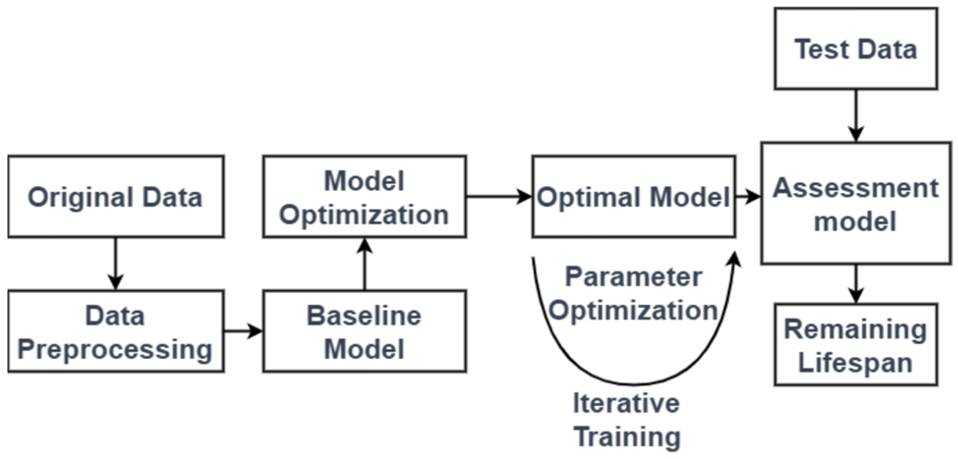
4.2. Prediction Process Based on the Autoformer Model

This paper employs the Autoformer model for predicting the lifespan of optical cables. The proposed forecasting approach is primarily divided into two segments: data preprocessing and model construction, with the specific workflow illustrated in Figure 2.

• Data Preprocessing: This study utilizes measured meteorological data from January 2011 to December 2023 in Guangzhou, including daily maximum and minimum temperatures and wind speed. Subsequently, leveraging the daily average temperature and wind speed, the corresponding optical cable lengths are calculated using a dedicated formula. For anomalous values, the Lagrange interpolation method is employed for estimation and imputation.
• Model Construction: The model is constructed following the architectural schematic of Autoformer, with input comprising the processed data and labels representing the residual lifespan at that time step. The output is a time series for the remaining lifespan prediction.
• Model Training and Testing: The model is trained on the training dataset and then evaluated on a separate test dataset.

5. Analysis of Cable Life Prediction Model Based on Autoformer

5.1. Comparison of Cable Life Prediction Model Results

Predicting the lifespan of fiber optic cables demands a rigorous model assessment. This paper utilizes root mean square error (RMSE), mean absolute error (MAE), and mean square error (MSE) as pivotal metrics to gauge the accuracy of predictive models against actual values.

In this paper, the optical cable information dataset was divided into training, validation, and test sets in a 4:1:1 ratio to ensure comprehensive coverage across different data distributions for model training, validation, and evaluation. During the experimental process, the model was configured to utilize a time window of 60 days as input, employing data from the past 60 days as input to capture the historical change trends in cable length. The encoder and decoder layers were set to two and one layers, respectively, balancing model complexity with the effective learning of data features and dependencies. The d_model was set to 4, correlating with the count of autocorrelation coefficients, to capture the temporal relationships in sequence data while ensuring computational efficiency. The learning rate was set to 0.0001, with 15 training epochs and a batch size of 16, to ensure stable model convergence during training and minimizing the occurrence of overfitting. To ensure the fairness and validity of the experiment, the configurations for the comparison models were kept identical to those of the proposed model. The comparative analysis results, as depicted in

Table 1. Performance metrics for different models.

Model	RMSE	MAE	MSE
LSTM	1.3184	1.0828	1.7383
Bi-LSTM	1.2361	0.9582	1.5278
Bi-LSTM + Attention	0.9131	0.7321	0.8338
Autoformer	0.5893	0.3687	0.3473

, reveal that the model proposed in this paper outperforms the comparative models across three evaluative metrics. Compared to the Bi-LSTM + Attention model, the Autoformer model achieved reductions in the RMSE, MAE, and MSE metrics by 35.46%, 49.63%, and 58.34% respectively.

Figure 3 illustrates a comparison of forecast results for changes in optical cable lengths in 2023 within the test set between the Autoformer model and comparison models. As can be observed in Figure 3, each model is proficient in accurately predicting future information, with a minor deviation from the actual data. This indicates that the models are proficient in mining time series sequences, effectively and precisely forecasting future trends in cable length variations. Notably, the Autoformer model proposed in this paper achieves a better fit in its predictions compared to actual values, displaying heightened predictive accuracy. Furthermore, the Autoformer model’s smooth and coherent prediction line overall suggests its stability and consistency in analyzing and projecting optical cable lifespan, particularly manifesting this trend when the data span a broader time range.

It is important to note that the chosen values for the time window length and d_model are based on our understanding of the problem and the experimental results presented in this study. These values may not be optimal for all scenarios, and further investigation and fine-tuning may be required for specific applications.

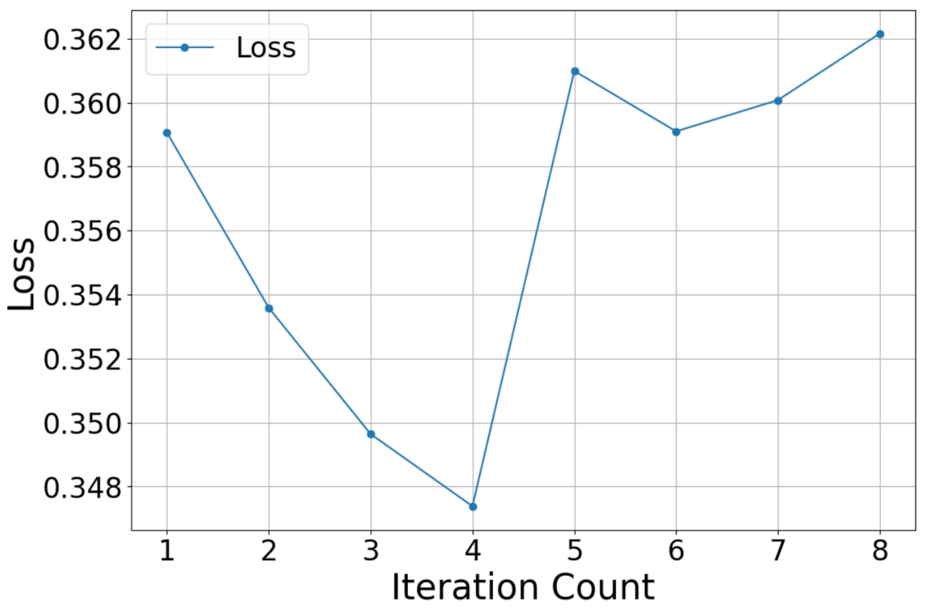
5.2. The Impact of Iteration Count on the Performance of the Autoformer Model

The iteration count reflects the decrease in the loss function of deep learning models and their convergence status. Utilizing MSE as the loss function, as demonstrated in Figure 4, the predictive performance of the Autoformer model markedly improves, with an increase in iteration count during parameter adjustment experiments. When the iteration count reaches 4, the model has already converged optimally. However, further training beyond this point not only fails to enhance the model’s predictive accuracy but also significantly diminishes it. This phenomenon suggests that the model might be overfitting the training data, losing its ability to generalize to new data. This attests to the Autoformer model’s robust parallel computing capacity in feature extraction, facilitating faster convergence. Considering the training time and computational costs, this study sets the iteration count for the model at 4.

5.3. The Impact of Learning Rate on the Performance of the Autoformer Model

The learning rate is a crucial factor in deep learning, directly impacting the convergence and speed of the optimization process. A learning rate that is too small can result in a slow convergence process, thereby extending the training time. Conversely, an excessively large learning rate may hinder convergence. As depicted in

Table 2. Evaluation metrics for different learning rates.

Learning Rate	RMSE	MAE	MSE
1 × 10−3	0.6091	0.3711	0.3535
5 × 10−5	0.6088	0.3707	0.3496
2.5 × 10−5	0.5893	0.3687	0.3473
1.25 × 10−5	0.6141	0.3771	0.3609
6.25 × 10−6	0.6186	0.3827	0.3591
3.125 × 10−6	0.6121	0.3746	0.3601

, the predictive efficacy of the Autoformer model, as measured by MSE, exhibits a non-linear relationship with the learning rate: while decreasing the learning rate initially improves model performance by allowing for more precise convergence, learning rates below 2.5 × 10⁻⁵ lead to prolonged training times and ultimately overfitting, as evidenced by the increasing MSE observed on the validation set when the learning rate falls below 2.5 × 10⁻⁵. Therefore, this study adopts the optimal learning rate of 2.5 × 10⁻⁵, which balances model accuracy and training efficiency.

5.4. The Impact of Time Window Length on the Performance of the Autoformer Model

The time window length is a crucial parameter that can significantly affect the performance of time series forecasting models. To delve into the effect of the time window on model efficacy, this experiment employed models trained over various window lengths for comparative analysis.

Figure 5 illustrates the impact of time window length on the Autoformer model’s performance, as measured by RMSE, MAE, and MSE. Initially, increasing the time window length leads to improved performance, reaching an optimal point at a length of 60 days. However, further extending the time window results in performance degradation. This phenomenon can be attributed to two primary factors. Firstly, a wider time window may cause the model to overemphasize earlier data points, potentially neglecting the significance of more recent information. Secondly, larger time windows require processing a greater volume of data, which can increase the risk of overfitting. This is evidenced by the rising validation error observed with longer time windows, indicating a reduced ability to generalize to unseen data. Therefore, selecting an appropriate time window length is crucial for balancing model complexity and generalization capability.

Figure 6 presents the results of a similar experiment conducted with the Bi-LSTM + Attention model. As with the Autoformer model, when the input window is set to 60, the model achieves peak performance. However, deviating from this value leads to a decline in predictive accuracy, suggesting limitations in the model’s ability to capture long-sequence temporal features.

A comparison of the results depicted in Figure 5 and Figure 6 reveals that the Autoformer model demonstrates greater robustness to variations in time window length compared to the Bi-LSTM + Attention model. Both models exhibit performance degradation with time windows exceeding 90 days, but the decline in RMSE is significantly more pronounced for the Bi-LSTM + Attention model. This suggests that the Autoformer model is more adept at capturing long-range dependencies within time series data, a capability not as pronounced in the Bi-LSTM + Attention model. These findings provide further evidence supporting the suitability of the Autoformer model for optical cable lifespan prediction tasks.

6. Conclusions

Based on the results of our numerical experiments, this paper introduces a novel approach for predicting the remaining lifespan of optical cables utilizing the Autoformer model. The proposed model leverages deep learning and computational methodologies, utilizing temperature fluctuations, wind loads, and the cable’s residual length to predict the cable’s lifespan. Experimental results demonstrate that the Autoformer model outperforms other deep learning models, indicating its potential for accurate and reliable lifespan prediction. This research contributes a more effective method to the field of optical cable lifespan prediction, providing network operators and communication services with more accurate residual life predictions. This facilitates timely maintenance scheduling, reduces potential network failure risks, and ensures service continuity and stability. Furthermore, this work also offers enterprises more precise predictions of a cable’s remaining life, aiding in planning equipment maintenance and production scheduling, thereby enhancing production efficiency and equipment utilization. These contributions are significant not only in the academic sphere but also have a profound impact on industrial practices and commercial applications.

References

1. Grunvalds, R.; Ciekurs, A.; Porins, J.; Supe, A. Evaluation of Fibre Lifetime in Optical Ground Wire Transmission Lines. Latv. J. Phys. Tech. Sci. 2017, 54, 40–49. [Google Scholar] [CrossRef]
2. Burdin, V.; Andreev, V.; Bourdine, A.; Dashkov, M.; Nizhgorodov, A. Reliability and lifetime estimations for field-aged optical cable. In Proceedings of the Internet of Things, Smart Spaces, and Next Generation Networks and Systems: 20th International Conference, NEW2AN 2020, and 13th Conference, ruSMART 2020, St. Petersburg, Russia, 26–28 August 2020. [Google Scholar]
3. Burdin, V.A.; Nizhgorodov, A.O. Lifetime prediction algorithm for an optical cable of cable link under exploitation. In Proceedings of the Optical Technologies for Telecommunications, Bellingham, WA, USA, 22 May 2020. [Google Scholar]
4. Burdin, V.A.; Nikulina, T.G.; Praporshchikov, D.E. Method for predicting the lifetime of an optical cable after the maintenance cycle. In Proceedings of the Optical Technologies for Telecommunications, Bellingham, WA, USA, 25 July 2022. [Google Scholar]
5. Nizhgorodov, A.O. Simple Approximate Formula for Forecast of The Lifetime of the Optical Fibers of a Cable Communication Line. Infokommunikacionnye Tehnol. 2021, 19, 29–34. [Google Scholar]
6. Han, W.; Hao, C.; Kong, D.; Yang, G. Cable Temperature Prediction Based on RF-GPR for Digital Twin Applications. Appl. Sci. 2023, 13, 7700. [Google Scholar] [CrossRef]
7. Han, W.; Yang, G.; Hao, C.; Kong, D.; Dong, Y. A Data-Driven Model of Cable Insulation Defect Based on Convolutional Neural Networks. Appl. Sci. 2022, 12, 8374. [Google Scholar] [CrossRef]
8. Wu, H.; Xu, J.; Wang, J.; Long, M. Autoformer: Decomposition transformers with auto-correlation for long-term series forecasting. Adv. Neural Inf. Process. Syst. 2021, 34, 22419–22430. [Google Scholar]
9. Zhou, S.; Zhang, X.; Liu, J.; Zhang, Y.; Wei, P.; Wang, Y.; Zhang, J. Long-Term Prediction of Particulate Matter2.5 Concentration with Modal Autoformer Based on Fusion Modal Decomposition Algorithm. Atmosphere 2024, 15, 4. [Google Scholar] [CrossRef]
10. Borzycki, K. Influence of temperature and aging on polarization mode dispersion of tight-buffered optical fibers and cables. J. Telecommun. Inf. Technol. 2005, 30, 96–104. [Google Scholar] [CrossRef]
11. Günday, A.; Karlık, S.E. Optical fiber distributed sensing of temperature, thermal strain and thermo-mechanical force formations on OPGW cables under wind effects. In Proceedings of the 2013 8th International Conference on Electrical and Electronics Engineering (ELECO), Piscataway, NJ, USA, 28 November 2013. [Google Scholar]
12. Malyszko, O.; Zenczak, M. Current-carrying capacity of overhead power transmission lines in different weather conditions. In Proceedings of the XV International Symposium on Theoretical Engineering, Berlin, Germany, 22 June 2009. [Google Scholar]
13. Burdin, V.A. The method for a measurement of the excess fiber length on the cable delivery length by using the polarization reflectometry. In Proceedings of the Optical Technologies for Telecommunications, Bellingham, WA, USA, 6 April 2017. [Google Scholar]
14. Setayeshgar, A. Principles of Mechanical Design in Overhead Transmission Lines. Master’s Thesis, Aalto University, Espoo, Finland, 2016. [Google Scholar]
15. Li, Y.-Q.; Zhao, H.-W.; Yue, Z.-X.; Li, Y.W.; Zhang, Y.; Zhao, D.C. Real-Time Intelligent Prediction Method of Cable’s Fundamental Frequency for Intelligent Maintenance of Cable-Stayed Bridges. Sustainability 2023, 15, 4086. [Google Scholar] [CrossRef]
16. Ashfaq, A.; Chen, Y.; Yao, K.; Sun, G.; Yu, J. Microbending loss caused by stress in optical fiber composite low voltage cable. In Proceedings of the 12th International Conference on the Properties and Applications of Dielectric Materials (ICPADM), Xi’an, China, 20 May 2018. [Google Scholar]
17. Qin, J.; Gao, C.; Wang, D. LCformer: Linear Convolutional Decomposed Transformer for Long-Term Series Forecasting. In Proceedings of the International Conference on Neural Information Processing, Changsha, China, 20 November 2023. [Google Scholar]
18. Alrasheedi, F.; Zhong, X.; Huang, P.C. Padding module: Learning the padding in deep neural networks. IEEE Access 2023, 11, 7348–7357. [Google Scholar] [CrossRef]
19. Henry, M. An ultra-precise Fast Fourier Transform. Meas. Sens. 2024, 32, 101039. [Google Scholar] [CrossRef]
Figure 1. Autoformer architecture. The encoder eliminates the long-term trend–cyclical part by series decomposition blocks and focuses on seasonal patterns modeling. The decoder accumulates the trend part extracted from hidden variables progressively. The past seasonal information from encoder is utilized by the encoder–decoder auto-correlation.
Applsci 14 06286 g001
Figure 2. Prediction process.
Applsci 14 06286 g002
Figure 3. Comparison of predicted optical cable length changes in 2023: LSTM, Bi-LSTM, Bi-LSTM + Attention, and Autoformer Models. Actual values are shown in gray. The Autoformer model’s predictions are shown in red. Green, orange, and blue lines represent the predictions of the LSTM, Bi-LSTM, and Bi-LSTM + Attention models, respectively.
Applsci 14 06286 g003
Figure 4. Variation in loss with iteration count.
Applsci 14 06286 g004
Figure 5. Impact of time window lengths on Autoformer model performance.
Applsci 14 06286 g005
Figure 6. Impact of time window length on Bi-LSTM + Attention model performance.
Applsci 14 06286 g006