Optimization of Parametric Equalizer Filters in In-Vehicle Audio Systems with a Genetic Algorithm

Abstract

This study aims to automate the optimization of a full-range speaker in an SUV’s audio system according to the equal-loudness contours principle. The input signal and frequency responses of the amplifier and speaker were transferred to Matlab. Using ideal filter parameters, ten parametric equalizer models were created, and the speaker output was obtained using the convolution technique. The same filter settings were applied to the vehicle multimedia system, and the experimental results were obtained. The simulation and experimental results were compared, showing high similarity, with a Pearson correlation of 0.9295 and a root mean square error (RMSE) of 2.29. The results were compared with the ideal contour. The Pearson correlation coefficients for the simulation and experimental results were 0.6341 and 0.6715, with RMSE values of 4.88 and 2.57, showing low similarity. Consequently, each parametric equalizer filter’s parameters were optimized using a genetic algorithm. The genetic algorithm was executed thirteen times for robustness, and the best parameters were selected. The optimized parameters were applied to the multimedia system, and the results were compared with the ideal contour. The correlation coefficients for the simulation and experimental results were 0.9692 and 0.9675, with RMSE values of 1.17 and 1.34. These results indicate that optimization aligns the speaker output closer to the ideal contour, enhancing in-vehicle audio system performance and increasing users’ satisfaction.

1. Introduction

Listening to music while driving, one of the most common activities, not only serves as a source of entertainment for drivers and passengers but also significantly impacts driving comfort and overall fatigue levels. Studies demonstrate that in-car sound has a direct effect on the driver’s comfort and fatigue levels [1]. In this context, the quality of in-car sound emerges as a critical factor that influences substantially the experience of both drivers and passengers. With the advancement of technology, vehicle manufacturers and audio system designers develop various strategies to meet users’ expectations and improve the systems regarding sound quality, aiming to minimize driver fatigue.

The impact of in-car sound quality on the listening experience is evaluated within the framework of sound engineering and psychoacoustic principles [2]. Particularly, the compatibility of sound characteristics from speaker output with the equal-loudness contour, which reflects the human ear’s varying sensitivity to frequencies between 20 Hz and 20 kHz, is critical for the clarity and accuracy of sound [3]. The adequacy within this frequency range provides a detailed and rich audio experience, enhancing the comfort and enjoyment of drivers and passengers. Moreover, studies indicate that systems incompatible with the equal-loudness contour negatively affect drivers’ fatigue and stress levels during long-distance trips. This situation significantly impacts drivers’ attention and reaction times, thereby endangering overall road safety [4]. Therefore, optimizing in-car sound systems based on this contour plays a critical role not only in enhancing the driver and passenger experience but also in maximizing road safety.

In vehicle audio systems, it is required that the different frequency ranges be meticulously adjusted to ensure that the speaker output aligns with the equal-loudness contour. This tuning is carried out with equalizers that are used to adjust the level of sound signals within specific frequency ranges. There are three types of equalizers: graphic equalizers, parametric equalizers, and digital equalizers. The graphic equalizer allows users to adjust sound levels manually at predefined frequency bands. The digital equalizer, utilizing sophisticated technology, automatically adjusts the sound profile based on factors such as vehicle speed and engine noise, catering to advanced driver assistance systems. The parametric equalizer is a highly adjustable audio processing filter used to modify the amplitude of sound signals within certain frequency ranges. This filter provides precise control over three parameters: center frequency, gain, and quality factor (Q factor). The detailed control capability makes the parametric equalizer particularly suitable, compared to other options, for tuning the speaker output according to the equal-loudness contour, making it preferable in vehicle multimedia systems [5].

The in-car sound system is a complex structure comprising various components, such as the vehicle multimedia system, amplifiers, speakers, cables, and connectors. Although each component affects the frequency response throughout the system in various ways, the speakers make the most critical modifications. Since a single speaker cannot deliver perfect performance across all frequencies, quality sound systems employ speakers together, designed for different frequency regions. Modern vehicles include a wide variety of speakers such as subwoofers, woofers, mid-ranges, full-ranges, and tweeters. Each of these speakers offers different responses in specific frequency ranges; thus, in the optimization of vehicle audio systems, equalizer settings need to be meticulously addressed for all types of speakers [6].

In vehicle multimedia systems, tuning filter parameters to conform to the equal-loudness contour and measuring speaker output with a sound analyzer are fundamental steps in optimization. However, these steps are detailed and challenging due to their reliance on manual tuning and experimental methods and because repeated analyses are required to achieve optimal results. Additionally, the process of evaluating results through subjective observation makes it difficult to ensure the consistency in achieving desired acoustic levels [6].

Given that the equal-loudness contour spans a wide frequency range, multiple parametric equalizer filters are often used in vehicle multimedia systems for fine-tuning. Considering that each filter is controlled by three parameters, the optimization of in-car sound systems becomes a particularly cumbersome process, especially for different types of speakers. Therefore, the use of computer-aided modeling and simulation technologies for the optimization of multiple parametric equalizer filters holds the potential to enhance the efficiency and effectiveness of the design process of in-car sound systems. Particularly, the filter design possibilities provided by computer-aided mathematical modeling software, coupled with simulations conducted through signal processing techniques to calculate the system’s frequency response, and the assessment of conformity to the equal-loudness contour through statistical methods, both accelerate and simplify the optimization process of in-car sound systems. These modern approaches overcome the time and complexity issues encountered with experimental methods, offering the opportunity to perform detailed analyses necessary for perfecting the design and settings of in-car sound systems [7].

In addition to the previous processes, the use of intelligent algorithms during the tuning of filter parameters holds the potential to advance the optimization process. Methods such as metaheuristic algorithms and Artificial Neural Networks can be utilized to optimize the process of finding the most suitable filter combination for the equal-loudness contour, providing high levels of accuracy and efficiency in parameter selection. These intelligent algorithms, compared to manual trial-and-error methods, allow for the rapid and cost-effective achievement of the ideal frequency response, reducing time and resource usage in acoustic tuning [8].

This study aims to automate the process of adjusting the full-range speaker in the audio system of an SUV according to the equal-loudness principle. First, the input sound and the frequency responses of the speaker were transferred to the Matlab environment. Then, using the filter parameter values defined in the standards for the ideal hearing curve in 1/1 octave bands, ten parametric equalizers were modeled, and the speaker output was obtained using the convolution technique. The same filter settings were applied to the vehicle’s multimedia system, and the simulations were verified, obtaining experimental results. Following this step, the center frequency, gain, and Q factor of each parametric equalizer were determined using a genetic algorithm to achieve optimal acoustic performance. These filter parameters were iteratively optimized to match the ideal equal-loudness contour closely. After the optimization process, the calculated parameters were applied to the vehicle multimedia system, and the obtained experimental results were compared with the simulation results in the Matlab environment, using correlation and root mean square error analyses. A total of thirteen different experiments were conducted, and the results of each experiment were analyzed separately. This allowed for a detailed examination of the effectiveness of the modeling, simulation, and applied optimization strategy.

2. Literature Review

Several studies in the literature have demonstrated the effectiveness of genetic algorithms and other metaheuristic methods in the optimization of audio systems. Mishima and Kajikawa (2012) developed an automatic parameter adjustment method for audio equalizers using an interactive genetic algorithm (IGA). In their study, user satisfaction was evaluated by measuring the difference between the user-preferred frequency response and the optimized frequency response [9].

Prince and Kumar (2018) proposed a 16th-order IIR filter-based graphic equalizer design optimized using a genetic algorithm. In their study, they succeeded in improving filter performance by reducing the interference between adjacent frequency bands and maximizing gain. The average root mean square error (RMSE) value was reported as 0.05, and the maximum gain achieved was 12 dB [10].

Ogura and Wang (2020) demonstrated superior performance in IIR filter-based audio equalization using the Gravitational Search Algorithm (GSA), achieving lower error rates compared to traditional methods. The RMSE value was reported as 0.06, and the maximum gain was found to be 11 dB [11].

In these studies, the RMSE was used to measure the difference between the optimized frequency response and the target frequency response. Gain refers to the capacity of the filters to enhance the signal at specific frequencies.

This study differs from other studies in the literature in several key aspects. Previous studies have typically focused on users’ satisfaction or on achieving specific frequency responses. In this study, optimizations aimed at enhancing the performance of in-vehicle audio systems are conducted according to ideal hearing curves specified by standards. This ensures that the speaker output conforms more closely to the principle of equal loudness.

Additionally, while most studies in the literature primarily use the RMSE or mean square error (MSE) as performance metrics, this study also incorporates the correlation metric. Correlation is included to better analyze the similarity between the optimized frequency response and the ideal curve. This allows for a more comprehensive evaluation of how closely the speaker output matches the ideal curve.

3. Materials and Methods

3.1. Normal Equal-Loudness-Level Contours

The human ear has the ability to perceive sound waves at different frequencies; however, this perceptual capacity can vary significantly, depending on the frequencies. Fletcher and Manşon developed a chart, called the equal-loudness contours, based on their research and experimental studies on this subject. This chart was later standardized under the name ISO 226 Standard [12]. This standard includes the equal-loudness contours, which define the sound pressure levels required for sounds at different frequencies to be perceived as equally loud by the human ear. The equal-loudness contours for different phon levels are shown in Figure 1.

Equal-loudness contours were determined by taking as reference the frequency of 1000 Hz, which is well perceived by the human ear. These contours are specifically designed considering the psychoacoustic effects on humans. The contours are created based on the average responses of individuals aged between 18 and 25 years, who are considered otologically normal, forming an ideal ear model [12].

3.2. System Components and Modeling

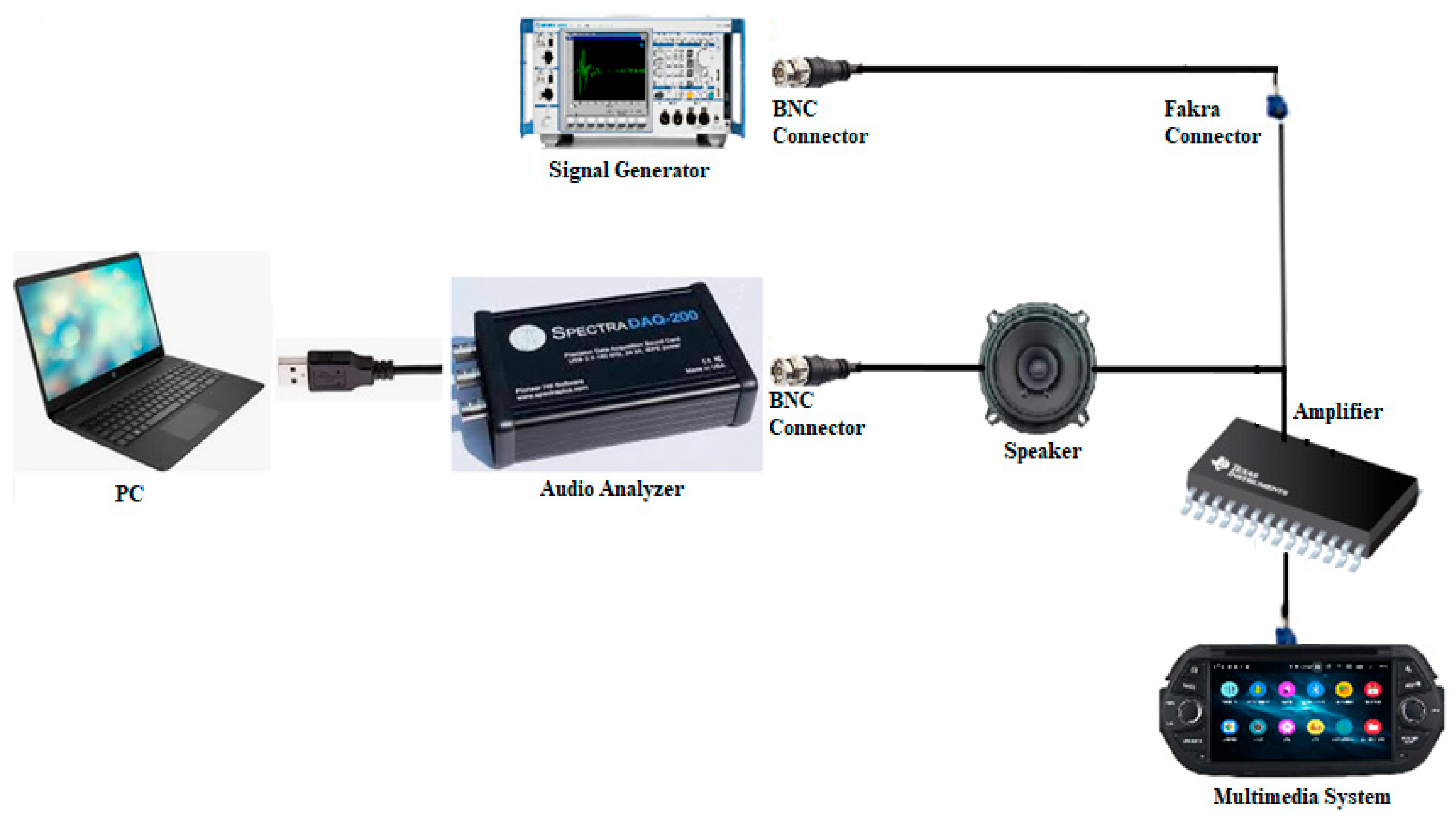
The in-vehicle audio system has a complex structure comprising multiple components. Key components include a signal generator, an audio analyzer, BNC connectors, a speaker, and a vehicle multimedia system. The transmission of signals starts with the input sound from the signal generator, traveling through BNC connectors to the audio analyzer, and then to the speaker. At the end of the signal process, the sound waves produced by the speaker are delivered to users via the in-vehicle multimedia system. These components are critical not only for the in-vehicle audio quality but also for directly influencing the auditory experience of drivers and passengers. The final output obtained in the vehicle audio system is the result of multiplying the frequency responses of the system components with each other. Therefore, the frequency response of each component is among the critical factors directly impacting system performance. The system diagram is shown in Figure 2. Subsequent sections will address the modeling of each component in terms of frequency response and examine the interactions between these responses.

(A)

Input Sound

White noise is frequently preferred in the calibration processes of sound systems because it has equal sound intensity in a wide frequency range, such as 20 Hz–20 kHz. This feature allows for objective testing of the system’s frequency response throughout the entire frequency band; thus, it enables a comprehensive analysis of system performance. Particularly in acoustic arrangements of sound systems and rooms, this broad-spectrum sound source is utilized to assess system performance and the necessary adjustments are implemented. Consequently, the responses of sound systems at various frequencies can be objectively measured and optimized.

A similar usage is found in in-vehicle sound systems. Thanks to its balanced and comprehensive frequency spectrum, white noise provides an ideal test signal for accurately detecting the frequency response of sound systems across a wide frequency range. A significant advantage is that during in-vehicle acoustic adjustments using white-noise signals, it is possible to interactively examine and adjust the effects of applied filters across all frequencies [6].

Acoustic analyzers use frequency weighting curves to simulate the human ear’s sensitivity to different frequencies. The A, B, and C weighting scales, displayed in Figure 3, represent various frequency response filters employed in sound measurements. The process of weighting adjusts the measured decibel (dB) values of sounds at specific frequencies to match the sensitivity levels perceived by the human ear at those frequencies. Given the human ear’s lower sensitivity to low frequencies and higher sensitivity to high frequencies, these weighting curves are essential for accurately reflecting perceived sound intensity. These curves aim to align the measured sound levels more closely with the natural response of the human ear and enhance the effective assessment of sound’s true impact. Therefore, weighting filters are applied to the white-noise signal used as the input sound.

A-weighting primarily represents the sensitivity of the human ear to ambient noise measurements at low sound levels. This scale is more sensitive between the frequencies of 500 Hz to 10 kHz, while it reduces sounds at lower and higher frequencies, making it ideal for everyday environmental sound measurements. B-weighting is designed for medium to high sound levels (80 to 90 phon) and emphasizes sounds across the frequency range slightly more, making it useful in environments such as cinema and music production. C-weighting is used at high sound levels and provides a flatter response across a wide frequency range. Thereby, low- and high-frequency sounds are measured at nearly their original levels. This achieved accuracy is especially required in industrial settings and at concerts [14].

B-weighting is a method designed to better reflect the sensitivity of the human ear at medium to high sound levels. Since it is necessary to regulate the system based on the mid to upper sound levels in setting vehicle sound systems, B-weighting, shown in Figure 3, which presents the frequency response from 20 Hz to 20 kHz, is used. In this context, our study is based on the equal-loudness contour at 1000 Hz, with an amplitude level of 90 dB, as shown in Figure 1. After applying the B-weighting process to the white-noise signal, the input audio used in this study is generated. The frequency response of this input sound is depicted in Figure 4.

(B)

Parametric Equalizer Filters

The parametric equalizer filter is a tool commonly used in audio processing and music production and has become a standard component in automotive multimedia systems. This filter adjusts the audio signal by targeting specific frequency ranges, thereby facilitating the adjustment of the sound’s tonal balance. The parametric equalizer is adjusted based on three primary parameters: center frequency ($f_0$), bandwidth (or $Q$ factor), and gain ($G$). The gain modifies the intensity of the sound signal by increasing or decreasing the amplitude within the selected frequency band. The bandwidth determines the range of frequencies where the filter is effective, and it is usually expressed in octaves. The $Q$ factor is defined as the inverse of the ratio of the bandwidth to the center frequency and indicates the sharpness of the filter. A high $Q$ factor means a narrower bandwidth and a sharper filter response. These parameters allow users to finely tune how narrowly or broadly they want to affect a specific frequency, thereby precisely achieving the desired sound characteristics.

The parametric equalizer is a crucial tool in audio processing, primarily incorporating various filter types such as peaking (bell), shelving, and notch filters. In vehicle multimedia systems, the peaking filter is particularly favored. This filter facilitates the adjustment of in-vehicle sound systems in, accordance with the principle of equal loudness, through its advantages, such as frequency adjustment flexibility, tone control, and focused frequency intervention. The peaking filter is designed to either emphasize or attenuate signals within a specific frequency band and plays a critical role in sound processing and equalization [15].

The mathematical model of the peaking filter is represented by a transfer function $H\left(f\right)$ that describes its effect on the frequency domain of the signal. This transfer function defines the relationship between the input and output of the signal as a function of frequency and is commonly formulated as (1)

$$H\left(f\right)=1+{\displaystyle \frac{GQ\left(\frac{f}{f_0}-\frac{f_0}{f}\right)}{1+Q\left(\frac{f}{f_0}-\frac{f_0}{f}\right)}}$$

(1)

Here, $f$ represents the frequency under study, $f_0$ is the center frequency (the frequency to be emphasized or attenuated), $G$ denotes the gain (in amplitude level, measured in dB), and $Q$ represents the quality factor (which inversely defines the bandwidth of the filter) [5].

According to the principle of equal loudness, the precise regulation of different frequency bands is necessary. Therefore, multiple parametric equalizer filters are generally used. The ISO 226:2003 standard [12] defines the characteristics of parametric filters required to achieve an ideal equal-loudness contour. Adjusted according to this standard, ten parametric filters were designed to provide optimal sound correction with corresponding gain and Q factor values at the specified frequencies. Each of these filters is set according to the frequency, gain, and Q factor values detailed in

Table 1. ISO_226_2003 norm equal-loudness contour filter values.

Center Frequency Values (Hz)	Gain Values (dB)	Q Factor Values
55	10.4	0.9
71	11.2	0.6
125	−2.4	0.7
250	−2.4	0.7
500	−1.2	0.7
1060	7.5	1.0
1280	2.0	0.9
3220	−10.0	1.0
6400	10.5	1.9
8100	9.5	2.0

.

In this study, ten parametric equalizer filters have been utilized to ensure an ideal sound experience in vehicle multimedia systems. A filter order of 12 was chosen, which is aligned with the order of existing filters in in-vehicle multimedia sound systems. The filters were created using the fdesign.parameq function, which is available in the DSP System Toolbox library of Matlab R2021b (9.11.0.1769968 version) software, and allows users to design a parametric equalizer filter with specified parameters.

(C)

Amplifier

Amplifiers serve as fundamental power-boosting devices in sound systems. In vehicle multimedia systems, amplifiers increase the amplitude of the received audio signal, enabling speakers to produce sound at higher volumes and with higher quality. This improves the signal-to-noise ratio (SNR), enhancing the clarity and detail of the sound while minimizing distortions.

Among in-vehicle entertainment systems, Class-D amplifiers are particularly preferred. These amplifiers are advantageous due to their high energy efficiency and quality sound output. Class-D amplifiers process audio signals in digital format, amplifying them directly, without converting them back to analog signals. This process allows them to achieve high sound levels with lower energy consumption, compared to traditional analog amplifiers. Additionally, these amplifiers provide a balanced and consistent response across a wide frequency range, making them ideal for music and sound effects [16]. In this study, an amplifier suitable for 4-ohm speakers was selected. Figure 5 details the frequency response of the chosen amplifier at 4 ohms.

(D)

Speaker

Speakers function as the final output component of sound systems; they convert filtered and amplified audio signals into physical sound waves and deliver them to listeners.

The types of speakers used in vehicle sound systems are specially designed to provide optimal performance across different frequency ranges. Essentially, these speakers are categorized into four main types to cover low, mid, and high frequencies: subwoofer/woofer, mid-range, tweeter, and full-range speakers. Each type of speaker is optimized for a specific frequency range, and the frequency ranges of these speakers are detailed in

Table 2. Frequency ranges of speakers.

Speaker Type	Frequency Range
Subwoofer	20 Hz–200 Hz
Woofer	04 Hz–500 Hz
Mid-Range	250 Hz–4000 Hz
Tweeter	2000 Hz–20,000 Hz
Full-Range	80 Hz–12,500 Hz

[6].

The type of speaker used in this study is the full-range speaker, which covers a wide frequency range. Figure 6 shows the frequency response of the full-range speaker. The manufacturer states that the effective operating frequency of this speaker is between 85 Hz and 12.5 kHz. This wide frequency range indicates that the speaker can adequately produce both low-frequency bass sounds and high-frequency treble sounds. In this study, the modeling of the speaker was based on this frequency response curve.

3.3. Modeling and Optimization of System Output

In this study, to ensure an ideal audio experience in vehicle multimedia systems, the processes of signal processing, filtering, integration of amplifier, and speaker responses were detailed, and the combined effect of these components was optimized. While creating the system model, a B-weighting white-noise signal was used as the input signal, followed by the integration of parametric equalizer filters, amplifier, and speaker components, sequentially. This integration is based on the cascading method, where the output of each system component serves as the input for the next component. This method allows for the step-by-step processing of the signal and the sequential application of each component’s effect.

In this cascading process, the role of convolution, one of the fundamental concepts of signal processing theory, is of great importance. Convolution, as a mathematical operation, involves applying a system response (e.g., the frequency response of an equalizer filter or an amplifier) to an input signal. This process is essentially performed by “folding” each point of the input signal with the system response and summing the results.

The convolution theorem explains the frequency domain representation of this process: the convolution of two signals (input and system response) in the time domain is equivalent to the multiplication of these signals in the frequency domain. This transformation is shown in (2).

$$y\left(t\right)=x\left(t\right)\ast h\left(t\right)={\int }_{-\infty }^{\infty }x\left(\tau \right)h\left(t-\tau \right)d\tau \leftrightarrow Y\left(f\right)=X\left(f\right)H\left(f\right)$$

(2)

Here, $y\left(t\right)$ represents the output signal in the time domain, $x\left(t\right)$ denotes the input signal in the time domain, and $h\left(t\right)$ represents the system’s impulse response in the time domain. The variable $\tau$ signifies the time at which the $x\left(t\right)$ signal is shifted over the $h\left(t\right)$ signal. In the frequency domain, $Y\left(f\right)$ represents the output signal, $X\left(f\right)$ denotes the input signal, and $H\left(f\right)$ is the system’s frequency response.

This property allows engineers and designers in the field of signal processing, particularly in filter design and audio processing applications, to perform complex signal processing operations more efficiently. In this study, since the system components were modeled in the frequency domain, the convolution operation was also performed in this domain [17].

To model the resulting signal at the system output, the amplitude responses of the input signal, amplifier, and speaker components described in Figure 4, Figure 5 and Figure 6 were first imported into Matlab. Since the signals were defined in the frequency domain, the frequency responses of the parametric equalizer filters were calculated using the “freqz” function, and their amplitude responses were obtained. Here, a sampling frequency of 96 kHz, which is also used in the actual setup, was employed. The convolution of these obtained signals was performed by multiplication, as shown in Equation (2), and the speaker output was modeled.

In this study, statistical analyses were used to measure the performance by comparing the experimental results obtained from the speaker output. Pearson correlation analysis and RMSE methods were utilized for this purpose.

Pearson correlation analysis is a statistical method used to measure the linear relationship between two data sets. This analysis helps determine how two variables change together, producing a correlation coefficient (r) between −1 and 1. A correlation coefficient close to 1 indicates a strong positive linear relationship, while a value close to −1 indicates a strong negative linear relationship. A value near 0 suggests no relationship between the two data sets. In this study, Pearson correlation analysis was used to examine the linear relationship between the obtained results. The Pearson correlation coefficient is calculated using (3).

$$r={\displaystyle \frac{n\sum \left(xy\right)-\sum x\sum y}{\sqrt{\left[n\sum x^2-\sum {\left(x\right)}^2\right]\left[n\sum y^2-\sum {\left(y\right)}^2\right]}}}$$

(3)

Here, x and y refer to the data sets, and n refers to the total number of data points.

The RMSE is a method used to measure the magnitude of differences between two data sets. The RMSE evaluates the deviations among the obtained results and quantitatively indicates the amount of error. A low RMSE value indicates that the results are close to each other. RMSE is calculated using (4).

$$\sqrt{{\displaystyle \frac{1}{n}}{\sum }_{i=1}^n{\left(y_i-x_i\right)}^2}$$

(4)

These statistical analyses played a critical role in evaluating the agreement between the ideal contour and the experimental and simulation results. While Pearson correlation analysis determined the linear relationship between the results, RMSE analysis quantitatively measured the accuracy of this relationship [18].

To align the signal output from the speaker with the ideal contour given by the equal-loudness principle, the optimization of filter parameters was performed. Metaheuristic algorithms were preferred for the optimization. Metaheuristic algorithms are methods capable of conducting effective and efficient searches over large solution spaces and are not specific to a particular problem. In this study, the genetic algorithm (GA), one of the metaheuristic algorithms, was chosen.

The GA is an optimization technique based on the principles of biological evolution and operates on solution sets called chromosomes. Initially, an initial population consisting of random solutions is created. Then, the fitness of each solution is evaluated according to a specific objective. Solutions with higher fitness values are selected to have greater representation in subsequent generations. Crossover operations are performed among the selected solutions to create new solutions (offspring), and small random changes (mutations) are applied to the solutions obtained from the crossover. Finally, the population is updated with the new solutions, and the process is repeated until a certain fitness value is achieved, or a specified number of iterations is reached [19].

Genetic algorithms have the capability to operate effectively in large and complex solution spaces. In terms of flexibility and adaptability, genetic algorithms can be tailored to various optimization problems and provide flexibility for different objectives [20]. Given the numerous frequency and parameter combinations in vehicle audio systems, genetic algorithms are ideal for addressing such problems.

In this study, a GA was implemented using the “optimoptions” and “ga” functions from Matlab’s Global Optimization Toolbox. The GA was configured with a population size of 100 individuals. Thus, 100 different solutions were evaluated in each generation, and it allowed for a more comprehensive exploration of the solution space. The algorithm was allowed to run for a maximum of 50 generations, ensuring that the algorithm had sufficient time to search for an optimal solution, while keeping the computation time under control.

The success of the GA depends on the careful selection of various parameters. In this study, the crossover rate was set to 0.8. This rate helps maintain genetic diversity while allowing successful traits to be passed on to the next generation. Additionally, uniform mutation was chosen as the mutation function, and the mutation rate was set to 0.2. This enables the algorithm to avoid local minima and explore a broader solution space.

The selection function used was stochastic uniform selection. This method increases the probability of selecting individuals based on their fitness values, allowing better-performing solutions to be more represented in the next generation. Arithmetic crossover was used as the crossover function. This method combines the genetic information of the parents to create new individuals, facilitating the discovery of better solutions.

In the application of the GA, the fitness function was determined by comparing the speaker output with the ideal contour. The fitness function was calculated using both the correlation and the RMSE values. Genetic algorithms inherently strive to minimize the fitness function. Therefore, if the correlation value was positive, the fitness function was calculated as the inverse of the correlation ($1/correlation$); if the correlation was negative, a penalty value was added. This approach ensures that the genetic algorithm works to increase the correlation, thereby decreasing the fitness value as the correlation becomes more positive. Additionally, the RMSE value was incorporated into the fitness function, ensuring that a smaller RMSE results in more similar outcomes. This method has helped the speaker output to become closer to the ideal contour, thereby enhancing the performance of in-vehicle audio systems.

The genotype representation is achieved by encoding the speaker filter parameters as a series. Each genotype is a vector containing the values of center frequency, gain, and Q factor. The genotype is coded to include three parameters for each filter, as shown in (5).

$$genotype=\left[f_1, G_1,Q_1, f_2, G_2,Q_2,\dots ,f_{10}, G_{10},Q_{10}\right]$$

(5)

The genotypes used in this study were determined within the lower and upper bounds, specified by the ISO 226:2003 standards and listed in Table 1. These bounds aim to bring the filter parameters closer to the ideal contour. The lower bounds ($l_b$) and upper bounds ($u_b$) for the first to the tenth filter are provided in

Table 3. Lower and upper limit values for genotype filter parameters.

Center Frequency Values (Hz)		Gain Values (dB)		Q Factor Values
${\mathit{l}}_{\mathit{b}}$	${\mathit{u}}_{\mathit{b}}$	${\mathit{l}}_{\mathit{b}}$	${\mathit{u}}_{\mathit{b}}$	${\mathit{l}}_{\mathit{b}}$	${\mathit{u}}_{\mathit{b}}$
52	64	8.0	12.0	0.7	1.1
64	102	8.0	12.0	0.5	0.8
102	160	−3.5	−0.5	0.8	1.2
200	340	−3.5	−0.5	0.6	0.9
440	640	−2.5	−0.5	0.6	0.9
850	1100	6.0	10.5	0.8	1.2
1100	1400	0.5	4.0	0.8	1.1
2850	4250	−12.0	−8.0	0.8	1.2
5700	6800	8.0	12.0	1.6	2.1
7600	9400	7.5	11.5	1.7	2.2

.

The computational complexity of the genetic algorithm depends on the population size and the number of generations. The parameters used in this study were carefully selected to maintain control over the computation time while ensuring sufficient diversity and performance. These parameters maximize the flexibility and adaptability of the GA, creating an ideal environment for optimizing the frequency response of in-vehicle audio systems. Consequently, a higher quality and more comfortable audio experience is achieved for both drivers and passengers.

4. Results

First, the parametric equalizer filter parameters defined by the standards for equal loudness given in Table 1 were applied to the modeling software created to calculate the speaker output. The resulting speaker output contour is shown in Figure 7. Here, the blue line represents the simulation results, while the black line represents the ideal contour taken from the principle of equal loudness, with the effective frequency range of the speaker highlighted.

Subsequently, the experimental setup shown in Figure 8 was established to create the test environment. This experimental setup was also intended to evaluate the degree of alignment between the modeling and simulation results with a real-world application and to measure the performance of the simulation model.

In the test setup, the same filter parameters were loaded into the vehicle multimedia sound system, and the speaker output was measured. The simulation and experimental results are presented together in Figure 9 and compared with the ideal contour. Here, the blue line represents the simulation results, the red line represents the experimental results, and the black line represents the ideal contour.

First, the experimental and simulation results were compared for the effective frequency range of the speaker to evaluate the performance of the simulation model. For this purpose, Pearson correlation analysis and root mean square error (RMSE) calculations were performed. The correlation coefficient between the experimental and simulation results was found to be 0.9295. This result indicates a high degree of similarity, and it demonstrates the success of the simulation model. Due to the unknown frequency responses of the cables, vehicle multimedia system, and audio analyzer, these factors were not included in the models, and this situation affected the similarity. The RMSE value was calculated as 2.29. Attenuations caused by the elements and cables of the experimental setup created differences in amplitude values, which impacted the root mean square error rate.

Subsequently, the simulation results and experimental results were compared with the ideal contour. The Pearson correlation coefficient for the simulation and experimental results was found to be 0.6341 and 0.6715, respectively. The RMSE values were calculated as 4.88 and 2.57, respectively. As seen from the results, despite applying the ideal filter values, high similarity results were not achieved with the ideal contour. As shown in Figure 6, the speaker response is more sensitive to certain frequencies, causing deviations in amplitudes, which affected the overall system performance and reduced the similarity to the ideal contour.

Following these processes, the parametric equalizer parameters were calculated using a genetic algorithm-based optimization algorithm. The genetic algorithm was executed thirteen times to ensure the robustness and reliability of the results. Each run involved evaluating the best, worst, and average fitness values to comprehensively assess the optimization process.

The results of the genetic algorithm runs are summarized in

Table 4. Summary of genetic algorithm runs.

Run No	Best Fitness Value	Worst Fitness Value	Average Fitness Value
1	3.7278	6.4818	5.2462
2	3.9119	6.9003	5.2295
3	3.7849	6.8531	5.3337
4	3.1401	5.3548	4.264
5	3.3135	5.6533	4.4497
6	2.9103	5.2361	4.1722
7	3.6962	5.9486	4.7816
8	2.7229	3.9947	3.3807
9	2.2826	3.8436	3.0773
10	2.9983	4.1829	3.6482
11	2.7693	4.0229	3.3233
12	2.6523	3.8888	3.2189
13	2.6621	3.9380	3.3037

, which shows the best, worst, and average fitness values for each run. These values demonstrate the consistency and effectiveness of the genetic algorithm in optimizing the filter parameters.

The results indicate that the genetic algorithm effectively optimized the filter parameters, as seen in the range of best, worst, and average fitness values across the thirteen runs. The best fitness value of 2.2826 was achieved in run 9, demonstrating the algorithm’s ability to find highly optimized solutions. Conversely, the worst fitness value of 6.9 was observed in run 2, indicating some variability in the optimization process. Overall, these results demonstrate the algorithm’s capability to consistently find good solutions within the defined solution space.

In addition, statistical analyses were performed to assess the consistency and reliability of the genetic algorithm’s performance by calculating the mean, standard deviation, and variance of these fitness values. The results are presented in

Table 5. Statistical analysis of fitness values.

Metric	Best Fitness Values	Worst Fitness Values	Average Fitness Values
Mean	3.1209	5.0999	4.1099
Standard Deviation	0.5226	1.1885	0.8421
Variance	0.2731	1.4126	0.7092

.

The statistical analysis provided in Table 5 highlights the genetic algorithm’s robustness. The low standard deviation and variance values across the best, worst, and average fitness metrics indicate that the algorithm consistently produces reliable and effective results. Particularly, the low best fitness values demonstrate that the genetic algorithm effectively optimizes the filter parameters, ensuring the speaker output closely aligns with the ideal contour. The high variance in the worst fitness values suggests that the algorithm occasionally produces less optimal results; however, the overall consistency remains high.

The obtained parameters were applied to the modeling software created to calculate the speaker output, and the simulation results were obtained. Additionally, the filter parameters were loaded into the vehicle multimedia sound system, and the speaker output was measured. In all measurements, the filter parameters providing the best fitness values were applied. To evaluate the performance of the model and algorithm, the correlation and RMSE between the simulation results and the ideal contour, between the experimental results and the ideal contour, as well as between the simulation and experimental results, were calculated within the effective operating frequency range of the speaker. The obtained findings are shown in

Table 6. Summary of genetic algorithms runs.

Run No	Simulation vs. Ideal Contour		Experimental vs. Ideal Contour		Simulation vs. Experimental
	Corr	RMSE	Corr	RMSE	Corr	RMSE
1	0.9315	3.17	0.9187	2..61	0.9846	1.07
2	0.9076	3.18	0.9302	5.09	0.9636	2.42
3	0.9106	2.49	0.894	3.51	0.9797	1.42
4	0.9432	2.39	0.9578	1.87	0.9767	1.11
5	0.9199	2.68	0.9277	1.97	0.9816	1.27
6	0.9410	2.35	0.9208	1.58	0.9818	1.76
7	0.9132	2.00	0.8906	2.57	0.9834	2.23
8	0.9448	1.49	0.9279	3.40	0.9826	2.31
9	0.9692	1.17	0.9675	1.34	0.9864	1.00
10	0.9420	1.73	0.9438	4.96	0.9619	3.82
11	0.9538	1.63	0.9442	4.48	0.9798	4.48
12	0.9609	1.54	0.9457	3.44	0.9825	4.30
13	0.9601	1.55	0.9447	3.54	0.9826	4.39

.

The Pearson correlation and RMSE values in Table 6 indicate the performance of the model and algorithm. The best overall performance was observed in run 9, consistent with the findings in Table 5. The best results in terms of fitness, as well as correlation and RMSE values, were obtained in run 9. The filter parameters optimized in this run provided the highest similarity to the ideal contour and the best agreement between the simulation and experimental results.

However, some differences between the simulation and experimental results were observed. These discrepancies can be attributed to factors not included in the model, such as the unknown frequency responses of the cables, vehicle multimedia system, and audio analyzer. These elements were not modeled, which affected the similarity between the simulation and the experimental results.

To illustrate the specific filter parameters that achieved these optimal results, the parameters obtained from run 9 are detailed in

Table 7. Parametric equalizer filter parameters obtained from optimization in run 9.

Center Frequency Values (Hz)	Gain Values (dB)	Q Factor Values
58	11.8	0.9
63	11.9	0.7
157	−0.5	1.0
338	−3.2	0.8
589	0.7	0.8
894	6.2	1.1
1163	7.1	0.9
3326	−11.7	0.9
6768	12.1	1.5
7792	11.3	1.6

.

The simulation and experimental results are presented together in Figure 10 and compared with the ideal contour. Here, the blue line represents the simulation results, the red line represents the experimental results, and the black line represents the ideal contour.

The Pearson correlation analysis and root mean square error (RMSE) calculations used in previous analyses were also applied to the simulation model and experimental setup after optimization. The correlation coefficient between the experimental and simulation results was calculated to be 0.9864, and the RMSE value was 1.00. According to the results of the analysis, the simulation and experimental results showed a high degree of parallelism, indicating that the simulation model is consistent with the experimental data and demonstrating the reliability of the model.

Subsequently, the simulation and experimental results were compared with the ideal contour. The correlation coefficient between the ideal contour and the simulation results was found to be 0.9692, with an RMSE value of 1.17. The correlation coefficient between the ideal contour and the experimental results was calculated to be 0.9675, with an RMSE value of 1.34. These results indicate that the filter parameters obtained after optimization provide a high similarity to the ideal contour.

The correlation coefficients approaching 1 indicate that both the simulation and experimental results have a strong linear relationship with the ideal contour after optimization. This demonstrates an increase in the accuracy and reliability of the model. The decrease in RMSE values shows that the filter parameters obtained after optimization yield close results to the ideal contour, and that amplitude deviations are minimized. Low RMSE values indicate a significant improvement in system performance and a reduction in the model’s error margin.

These results also demonstrate a significant improvement in the performance of the in-vehicle audio system. By bringing the speaker output closer to the ideal contour through optimization, a higher quality and more comfortable audio experience for drivers and passengers has been achieved. This shows that genetic algorithm-based optimization is an effective method for optimizing the frequency response of in-vehicle audio systems and for enhancing system performance in real-world applications.

5. Conclusions

This study aimed to automate the process of optimizing the full-range speaker in the audio system of an SUV according to the equal-loudness principle. First, the frequency responses of the speaker and the input sound were transferred to the Matlab environment. Using the filter parameter values defined in the standards for 1/1 octave bands, ten parametric equalizers were modeled, and the speaker output was obtained using the convolution technique. The same filter settings were applied to the vehicle multimedia system, and the experimental results were obtained. These experimental results were validated by comparing them with the simulations.

To achieve optimal acoustic performance, the center frequency, gain, and Q factor of each parametric equalizer were determined using a genetic algorithm. These filter parameters were iteratively optimized to closely match the ideal equal-loudness contour. After the optimization process, the calculated parameters were applied to the vehicle’s multimedia system, and the obtained experimental results were compared with the simulation results in the Matlab environment using correlation and root mean square error (RMSE) analyses. This allowed for a detailed examination of the effectiveness of the modeling, simulation, and applied optimization strategy.

First, the parametric equalizer filter parameters defined according to standard equal-loudness contour were applied to our modeling software, and the speaker output was calculated. Then, the same filter parameters were applied to the test setup, and the speaker output was measured. The simulation and experimental results were analyzed, yielding a Pearson correlation coefficient of 0.9295 and an RMSE value of 2.29. These findings indicate a high degree of similarity between the simulation and experimental results, demonstrating that the simulation model is consistent with the experimental data and performs successfully. The components not included in the model and attenuations from the test setup affected the correlation coefficient and the RMSE calculations. Subsequently, the results were compared with the ideal contour defined by the equal-loudness principle. The Pearson correlation coefficients for the simulation and experimental results were found to be 0.6341 and 0.6715, respectively, with RMSE values of 4.88 and 2.57. As understood from the results, despite using the ideal filter values, there was a low level of similarity with the equal-loudness contour. The used speaker was more sensitive to certain frequencies, causing deviations in amplitudes, which affected the overall system performance and reduced the similarity to the ideal contour.

Following the relevant analyses and tests, the parameters of the ten parametric equalizer filters were calculated using a genetic algorithm-based optimization software. The genetic algorithm was executed thirteen times to ensure the robustness and reliability of the results. Each run involved evaluating the best, worst, and average fitness values to comprehensively assess the optimization process. The calculated parameters were applied to both the modeling software and the test setup for computation and measurement.

The results of the genetic algorithm runs demonstrated the consistency and effectiveness of the algorithm in optimizing the filter parameters. Notably, the ninth run yielded the best overall performance, with a best fitness value of 2.2826, a worst fitness value of 3.8436, and an average fitness value of 3.0773. A high correlation and low RMSE values further validated the optimal performance achieved in this run. Specifically, the Pearson correlation coefficient between the simulation results and the ideal contour was 0.9692, with an RMSE of 1.17. The experimental results showed a Pearson correlation coefficient of 0.9675 and an RMSE of 1.34 when compared to the ideal contour. Additionally, the correlation between the simulation and the experimental results was 0.9864, with an RMSE of 1.00. These metrics indicate that the filter parameters optimized in this run provided the highest similarity to the ideal contour and demonstrated the best agreement between the simulation and the experimental results.

When comparing the updated results to the initial values, the Pearson correlation coefficient for the simulation results improved from 0.6341 to 0.9692, a significant improvement of 52.84%. The RMSE value for the simulation results decreased from 4.88 to 1.17, showing an improvement of 76.02%. Similarly, the Pearson correlation coefficient for the experimental results increased from 0.6715 to 0.9675, an improvement of 44.08%, while the RMSE value decreased from 2.57 to 1.34, an improvement of 47.86%. These improvements not only facilitate the real-world application of this study but also allow for making finer adjustments.

The results obtained after optimization indicate that the speaker output has been brought closer to the ideal contour, significantly improving the performance of the in-vehicle audio system. Both the simulation and experimental results demonstrate that the optimization effectively aligns the speaker response with the ideal contour, thereby providing a higher quality and more comfortable audio experience for drivers and passengers. These findings show that genetic algorithm-based optimization is an effective method for optimizing the frequency response of in-vehicle audio systems and enhancing system performance in real-world applications.

The proposed genetic algorithm-based approach offers several advantages over traditional methods. By focusing on the ideal hearing curve defined by standards, our method ensures a more accurate alignment with human auditory perception. Unlike most existing methods, which optimize filters based on user satisfaction or specific frequency responses, our approach provides a comprehensive evaluation, using both RMSE and correlation metrics. This dual-metric analysis allows for a more thorough assessment of the similarity between the optimized frequency response and the ideal curve, resulting in a higher quality audio experience.

However, there are also some limitations to our approach. The genetic algorithm can be computationally intensive, especially with large population sizes and many generations, which can lead to longer processing times. Additionally, fine-tuning the genetic algorithm parameters requires expertise and can be complex. The stochastic nature of genetic algorithms can also result in variability in the outcomes, necessitating multiple runs to ensure robustness and reliability. Furthermore, the need for extensive simulations and experiments to validate the algorithm’s effectiveness can be resource-intensive.

These findings underscore the significance and innovation of our approach in enhancing in-vehicle audio performance. Future work will focus on further refining the algorithm parameters and exploring additional optimization techniques to enhance the robustness and efficiency of the proposed method.

In future studies, it is recommended to better understand and include in the modeling some factors that were not considered in this study, such as the frequency responses of cables, the vehicle multimedia system, and the audio analyzer. Additionally, it is recommended that modeling and optimization studies be planned using a genetic algorithm to bring the ideal contour closer to the head region of the driver’s seat.

In conclusion, this study demonstrates the effectiveness of a genetic algorithm-based approach for optimizing the speaker output according to the equal-loudness contour. It shows the potential to achieve higher performance and users’ satisfaction in in-vehicle audio systems.