Adaptive Feature Refinement and Weighted Similarity for Deep Loop Closure Detection in Appearance Variation

Abstract

Loop closure detection (LCD), also known as place recognition, is a crucial component of visual simultaneous localization and mapping (vSLAM) systems, aiding in the reduction of cumulative localization errors on a global scale. However, changes in environmental appearance and differing viewpoints pose significant challenges to the accuracy of the LCD algorithm. Addressing this issue, this paper presents a novel end-to-end framework (MetricNet) for LCDs to enhance detection performance in complex scenes with distinct appearance variations. Focusing on deep features with high distinguishability, an attention-based Channel Weighting Module(CWM) is designed to adaptively detect salient regions of interest. In addition, a patch-by-patch Similarity Measurement Module (SMM) is incorporated to steer the network for handling challenging situations that tend to cause perceptual aliasing. Experiments on three typical datasets have demonstrated MetricNet’s appealing detection performance and generalization ability compared to many state-of-the-art learning-based methods, where the mean average precision is increased by up to 11.92%, 18.10%, and 5.33% respectively. Moreover, the detection results on additional open datasets with apparent viewpoint variations and the odometry dataset for localization problems have also revealed the dependability of MetricNet under different adaptation scenarios.

1. Introduction

Visual simultaneous localization and mapping (vSLAM), which simultaneously reconstructs camera pose and scene structure from video inputs, is one of the critical autonomous positioning and navigation technologies in various areas [1]. As an essential component of vSLAM systems, loop closure detection (LCD) is designed to detect whether the autonomous mobile robot has returned to a previously visited location. LCD is also known as a place recognition process. An accurate LCD method can help introduce additional global geometric constraints for the back-end pose optimization to reduce trajectory drift over time [2]. However, it has two major challenges: (1) the same location looks different due to illumination changes and seasonal variations, and (2) different scenes look similar due to the presence of similar objects. Therefore, to achieve lifelong localization, LCD must overcome the above challenges to provide reliable detection results.

In a vSLAM system, the LCD works as an appearance-based image matching component to compare the similarity between current and previously captured images. If the similarity score surpasses a predefined threshold, the corresponding images are identified as having achieved loop closure. In most popular approaches, LCD algorithms have two key steps: feature extraction and similarity measurement [3].

Feature extraction is always a prerequisite for tasks such as keyframe extraction, tracking, positioning, and mapping. It has a decisive influence on the performance of higher-level tasks. Traditional appearance-based methods often follow the visual bag-of-words (BoW) approach [2], where image descriptors are quantized into visual word vectors using clustering algorithms. However, the utilization of traditional handcrafted features discards geometric and structural information to some extent, making it difficult to cope with challenges like illumination changes and appearance variations.

Fortunately, deep learning (DL) networks have recently made significant breakthroughs in computer vision. Many related studies have shown that deep features adaptively learned in a data-driven manner can provide more robust image representations under changing environmental conditions [4]. Therefore, the learning-based frameworks are intuitively applied to solve LCD problems [5]. The models based on convolutional neural networks (CNNs) are widely adopted for their outstanding performance and efficiency [6]. Although learning-based LCDs have shown promising performance in extracting robust features, few studies have focused on similarity measurement strategies. Moreover, many algorithms ignore the internal mutual constraints between the feature extraction and similarity measurement processes, resulting in a lack of systematic optimization of networks.

Therefore, this paper presents a novel end-to-end LCD method designed for complex scenes with distinct appearance variations. The approach employs an AlexNet-based feature extraction network (FEN) to capture high-level visual representations of images. In comparison to hand-crafted feature extraction methods, FEN demonstrates superior capability for perceiving complex environments by mining potential geometric and structural information within the image. Additionally, a self-attention component, Channel Weighting Module (CWM), is employed to extract higher-level features from regions of interest, effectively retaining key information for LCD. The Similarity Measurement Module based on the feature relationship of the patch-by-patch similarity matrix calculates the similarity of adaptive weighted, which improves the loop closure detection detection ability.Taking advantage of adaptive weighting, MetricNet focuses on the effective spatial patches for score estimation, achieving robustness for LCD in challenging environments with significant appearance variations. In summary, our main contributions are as follows:

• Dynamic feature selection with self-attention: A novel learning-based LCD framework, incorporating the Channel Weighting Module guided by the insight of inverse document frequency in BoW, is proposed to distill the distinguishable spatial cues and regions of interest.
• Adaptive weighted similarity measurement for appearance variation: To enhance detection accuracy, a weighted similarity score is generated in the Similarity Measurement Module to distinguish positive and negative pairs based on a patch-by-patch matrix.
• Comprehensive multi-dataset validation: MetricNet achieves appealing performance on three typical datasets with drastic illumination and seasonal changes. It also delivers reliable results in scenes with significant viewpoint variations and performs well in localization applications.

The rest of this paper is organized as follows: A brief introduction of related works is provided in Section 2. The theoretical derivation and implementation of the proposed method are detailed in Section 3. Experimental results are presented in Section 4, and the conclusion is drawn in Section 5.

2. Related Works

In vSLAM systems, many practical approaches have been proposed to exploit the similarity between keyframes to achieve correct loop closure detection. In this case, LCD is essentially an image matching problem that consists of two main steps: feature extraction and similarity measurement. Meanwhile, the challenges of LCD in long-term operation have garnered significant attention.

2.1. Feature Extraction

2.1.1. Hand-Crafted Feature Representation

Traditional handcrafted features are manually designed to extract specific image features, which are usually divided into two categories: local and global descriptors. Taking advantage of compact representation and computational efficiency, the methods implemented with global features can describe the image appearance using a single vector, e.g., BRIEF [7] and SURF [8]. Histogram statistics can also be used for global description, e.g., HOG [9]. In addition, BoW enables the holistic description of incoming images by aggregating quantized local features, known as visual words [10]. The work VLAD [11] combines local image descriptors into a vector representation. In addition, several classical unsupervised algorithms transform the original features into binary codes, such as ITQ [12], CBE [13], SGH [14], and UBEF [15].

However, there are some well-established methods for extracting local features, such as SIFT [16] and ORB [17]. LPM [18] aims to preserve the local neighborhood structures of these potential true matches. These handcrafted-based methods neglect latent geometric and structural information, making it difficult to cope with challenging situations such as intense illumination changes and dynamic environments.

2.1.2. Learned Feature Representation

The emergence of learning-based methods has accelerated the development of computer vision technologies. Feature extraction based on deep learning has achieved great success in image recognition, classification, and retrieval [19]. Many powerful models, such as AlexNet [20], VGG [21], and ResNet [22], have been used as the base architectures in LCD [23].

NetVLAD [24] applies soft assignment of VLAD descriptors to these clusters, making NetVLAD an end-to-end trainable architecture for visual place recognition using a triplet ranking loss function. CAE-VLAD-Net [25] can extract deep features from the input image data by utilizing the locally aggregated descriptor, the stacked auto-encoders, and the teacher-student training strategy. It detects loop closures on keyframes based on the Euclidean distances between the extracted features. FILD++ [26] can jointly extract global and local convolutional features using different scales and construct an incremental database using the global features to recommend potential loop closures to be evaluated using the local features. However, some experimental results have shown that FILD++ has some difficulties dealing with significant background changes caused by weather changes and perceptual aliasing.

In addition, perception information about surrounding objects can significantly elevate the performance of LCDs. In the cooperative perception and control-supported infrastructure-vehicle system (IVS) [27], environmental perception based on object detection and semantic information also improves the ability of connected autonomous vehicles (CAVs). Many cooperative perception methods rely on visual sensing data and output the object’s state, such as location and velocity. Therefore, it is necessary for the existing localization and IVS to use and enhance environmental perception. In loop detection tasks, the cognitive perception of infrastructure can be achieved by detecting image landmarks derived from image patches to describe the visual data. The LCD method WASABI [28] builds a descriptor for place recognition across seasons based on the wavelet transform of the semantic edges of the image. Impressive results have also been achieved with the idea of detecting salient regions in late convolutional layers. These regions of interest can be selected by applying an attention mechanism. The work of Chen et al. [29] selects the most salient regions by extracting unique patterns based on the responses of the strongest convolutional layers.

2.2. Similarity Measurement

To quantify the confidence that the robot is observing a previously mapped area, several comparison techniques have been proposed. Based on different map representations, they can be broadly classified into two categories: image-to-image and sequence-to-sequence.

2.2.1. Image-to-Image Matching

Image-to-image methods rely on an individual similarity score to make the decision. This similarity score is compared with a predefined hypothesis threshold to determine whether the query image is topologically related to the older image. The sum of absolute differences (SAD) and the euclidean or cosine distance are the most commonly used metrics to estimate the matching confidence between two image features. When global representations (either handcrafted or learned) are used, direct matching is a reasonable measure of similarity. However, when local features are extracted, probabilistic methods are employed. The FAB-MAP [10], a probabilistic approach to the problem of place recognition, is developed to explicitly account for perceptual aliasing in the environment. The patch-based method STA-VPR [30] proposes an adaptive dynamic time warping (DTW) algorithm to align local features from the spatial domain while measuring the distance between two images, which realizes viewpoint-invariant and condition-invariant place recognition.

2.2.2. Sequence-to-Sequence Matching

Conversely, sequence-to-sequence methods are typically based on the comparison of submaps. The members of the groups with the highest similarity scores are considered the loop-closing image pairs. SeqSLAM [5] calculates the best candidate matching location within each local navigation sequence. However, it is less robust to changes in viewpoint. The sequence processing model MCN [31] adapts hierarchical temporal memory (HTM) for mobile robot place recognition. However, MCN suffers from instability and long time consumption due to the utilization of randomization operations. To improve this, SMCN [32] simplifies MCN and combines it with intra-set similarity and novel temporal filters to excavate the temporal continuity in LCD.

2.3. Challenges of LCD and Role of Deep Learning

2.3.1. Appearance Variation and Dynamic Environment

In LCD problems, it becomes increasingly difficult to determine whether two images were taken at the same location when faced with environments with significant variations in appearance and dynamic objects. Many researchers have proposed CNN-based loop detection methods [33] to overcome the challenges of changing environmental conditions, such as illumination and seasonal changes.

Chen et al. [34] extract the high-level features from AlexNet and achieve image invariance by applying multi-scale deep feature fusion. The patch-based method SAES [35] develops a self-adaptive enhanced similarity metric to enhance the discriminative ability for appearance variations. Although it achieves competitive detection results, the image separation prior to feature extraction causes the method to ignore the spatial information between each patch. CALC2.0 [36] is trained to construct the global feature space, which is composed of local features encoding visual appearance, semantic information, and keypoint description based on the residual activations of different cells in convolutional feature maps. The addition of multiple pieces information certainly helps the model overcome appearance variations. The work of Schubert et al. [37] describes unsupervised learning methods for visual place recognition in discretely and continuously changing environments. They utilize PCA-based approaches and propose a novel clustering-based extension of statistical normalization.

In addition, semantic-based perception information can provide a higher degree of invariability. Many works have shown that the use of semantic information [33] can better address the problem in dynamic environments. PlaceNet [38] is a multi-scale deep auto-encoder network augmented with a semantic fusion layer for scene understanding that is designed to handle dynamic scenes full of moving objects.

2.3.2. Perceptual Aliasing and Viewpoint Variation

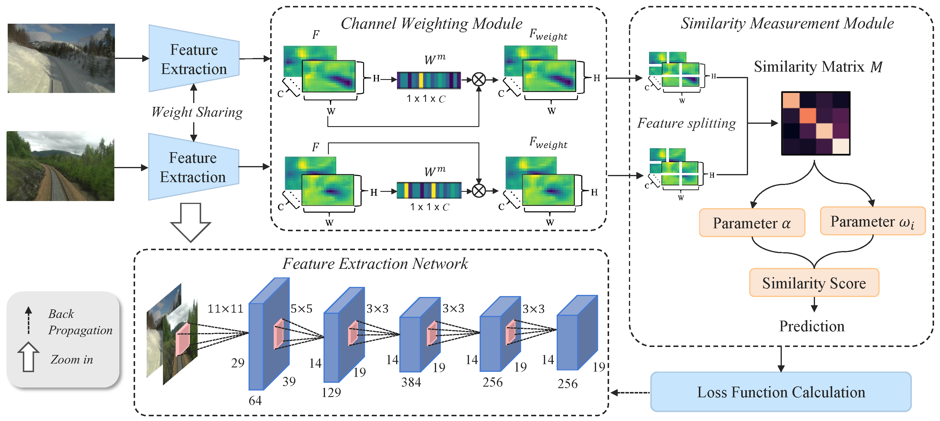
Furthermore, the occurrence of similar object appearances in different locations is termed “perceptual aliasing” problem [39]. Note that due to the similarity of visual words for loop measurements, BoW-based methods tend to produce false matches [40]. In this situation, instead of relying on image-to-image matching, LCD performance can be improved by incorporating multi-view information.

However, the change in viewpoint can range from minor to very dramatic. In general, ground robots tend to view the world from much the same viewpoints over repeated visits. However, the situation is much more complicated when the walking direction is opposite. Traditional loop closure detection systems may not provide satisfactory results in such scenarios. Some novel algorithms are designed to complement this by associating ground-to-air information [41]. The work of Jin et al. [42] designed a novel multi-tuplet cluster loss function to extract more discriminative feature vectors that are invariant to strong state changes and viewpoint changes. Semantic-based mapping techniques are typically used to achieve greater viewpoint robustness [43] in LCD. This infrastructure-based cognitive perception [27] can provide more effective information.

Both traditional and deep learning approaches mentioned above treat feature extraction and similarity measurement as two independent processes, relying on fixed distance metrics calculated from off-the-shelf features at the element level for matching. However, the effectiveness of similarity measurement is heavily influenced by the quality of the extracted features. Motivated by this, we propose a deep learning-based network that integrates feature extraction and similarity measurement as a well-coupled structure.

3. System Model

This section introduces the proposed framework (Figure 1) in detail.The main research idea of the paper is to jointly optimize the feature extraction and similarity calculation links and construct a similarity matrix to utilize the spatial information of the image to improve the detection performance in complex and changing scenes. The query and reference image pairs are taken as the input of our MetricNet. After the feature extraction network processing, we get the generated high-level visual representations. To achieve distinguishability in image descriptions, a self-attention component called the Channel Weighting Module is designed to extract the high-level features for regions of interest. Then the Similarity Measurement Module computes the patch-by-patch similarity matrix and obtains a value between 0 and 1 as the similarity of the pair of images to determine whether the two images are collected from the same location.

Inspired by SAES [35], MetricNet focuses on the spatial patches of image information. In SAES, the visual inputs are directly split into four patches and fed into feature extraction networks. However, this results in the truncation of objects near the visual center. While the implications for localization tasks may not be immediately apparent, such changes can compromise the integrity of image information and lead to false loop detections. In contrast, the learning-based feature extraction is applied to the entire input image in our method, and then the high-dimensional features are segmented into four patches. MetricNet adeptly maintains the information integrity, specifically accounting for the data along the boundaries of these patches.

The proposed method mainly incorporates three modules: Feature Extraction Network (FEN), Channel Weighting Module (CWM), and Similarity Measurement Module (SMM).

3.1. Feature Extraction and Distillation

3.1.1. Deep Feature Extraction

In LCD tasks, obtaining the ground truth for the dataset entails a substantial workload. Therefore, when training data are limited, it is crucial to efficiently utilize these data to train a model with strong generalization performance. The paper introduces the idea of transfer learning and fine-tunes the pre-trained network in an end-to-end manner on the existing limited training dataset, making the network more suitable for LCD tasks. This approach not only shortens the training time, promoting faster network convergence, but also enhances the generalization ability of the model.

To select the network with the best initial performance for the LCD task, this paper pre-screened the existing pre-trained networks. The selection method involved testing multiple networks on the same dataset and choosing the one that achieved the highest recall rate at 100% accuracy. As shown in Figure 2, AlexNet [20] achieved the highest recall rate at 100% accuracy, thus it was chosen as the feature extraction module.

The complete AlexNet network has five combined convolutional layers (including convolution, normalization, and max-pooling), three fully connected layers, and a subsequent softmax layer. The output of each layer of the AlexNet network can be extracted separately as the global features of the image, and as the network goes deeper, the ability of features to represent images is enhanced layer by layer. However, it has been demonstrated [6] that the features extracted from the fully connected layers cannot ideally characterize the image due to the loss of spatial information, as shown in Figure 3.

Therefore, as shown in Figure 1, this paper discards the subsequent fully connected and softmax layers of AlexNet and only preserves five combined convolutional layers (5CONVs) for our feature extraction. The details of the network structure are shown in

Table 1. Details of the feature extraction module.

Name	Type	OutputDim	Size	Stride
conv1	Conv	$64\times 59\times 79$	$11\times 11$	(4,1)
pool1	MaxPool	$64\times 29\times 39$	$3\times 3$	2
conv2	Conv	$192\times 29\times 39$	$5\times 5$	(1,1)
pool2	MaxPool	$192\times 14\times 19$	$3\times 3$	2
conv3	Conv	$384\times 14\times 19$	$3\times 3$	(1,1)
conv4	Conv	$256\times 14\times 19$	$3\times 3$	(1,1)
conv5	Conv	$256\times 14\times 19$	$3\times 3$	(1,1)

, including the settings of network type, output dimension, filter size, step size, and padding.

3.1.2. Channel Weighting Distillation

In imagery, different features have varying levels of discriminative importance. Ubiquitous elements, such as textureless walls, ground, and sky, are less distinguishable as they appear repeatedly in different scenes, making it difficult to complete LCD tasks based on them. Conversely, objects that are infrequent in the environment, such as traffic signs and landmarks, exhibit higher distinctiveness. Treating features extracted from different distinguishable parts equally can result in more false positives in loop closure detection. Therefore, more attention should be given to the parts with higher distinguishability among the features extracted from the image, while the importance of parts with lower distinguishability should be reduced.

Accordingly, to emphasize the imperceptible features of highly distinctive objects, we introduce a channel weighting mechanism in our FEN. Drawing inspiration from the approach in [44], we adopt a self-adaptive Channel Weighting Module (CWM), which is analogous to the Inverse Document Frequency (IDF) used in Bag-of-Words (BoW).In this context, a feature’s discriminability is inversely correlated with its frequency in the dataset. The less frequently a feature appears, the more important it becomes for classifying images. By calculating adaptive channel weights, we focus on low-frequency features that are more discriminative. The formulation of the CWM is defined as follows:

$$T_c={\displaystyle \frac{{\sum }_{h,w}^{F_{h,w}^c>0}1}{H\times W}}$$

(1)

$$W_c^m=\left\{\begin{array}{cc}\hfill log({\displaystyle \frac{{\sum }_{c=1}^C{T}_c}{T_c}}),& T_c>0\hfill \\ \hfill 0,& T_c=0\hfill \end{array}\right.$$

(2)

where $F\in R^{C\times H\times W}$ denotes the 3-dimension features calculated by FEN. $F^c\in R^{H\times W}$ is the feature map on the c-th channel of F, and $(h,w)$ index a feature pixel in $F^c$ as $F_{h,w}^c$. If $F_{h,w}^c>0$, this indicates a positive response of the feature pixel within the feature extraction network. After counting, $T_c$ represents the mean positive response of the c-th channel feature. To accentuate less conspicuous features, the self-adaptive attention mask $W_c^m\in R$ of the c-th channel is constructed using a $log$-based inverse function. This approach preferentially amplifies feature maps exhibiting lower responsiveness in the channel dimension. Based on that, our methodology facilitates selective feature enhancement.

Then we can derive the weighted feature map $F_{weight}\in R^{C\times H\times W}$ utilizing a self-attention mechanism across the channel dimension. The calculation process of $F_{weight}$ on the c-th channel can be described as

$$F_{weight,c}=W_c^m{F}^c$$

(3)

Since the calculation of channel-wise attention masks completely depends on the model’s response to visual features, there are no static trainable parameters in the self-attention mechanism. Therefore, CWM can dynamically obtain the channel-wise attention mask in a data-driven manner.

3.2. Similarity Measurement

Common similarity measurement methods based on local and global pixel-level descriptors often lead to misjudgments when dealing with scenarios where the appearance varies significantly at the same location or appears similar at different locations. To alleviate the aforementioned problem, this paper aims to leverage the spatial information of images to enhance the capability to handle variations in environmental appearance due to changes in lighting, weather, or seasons.

Taking advantage of the natural properties of the CNN convolution process that overlap each convolutional sliding window, all the context information at the patch boundaries is preserved. Unlike SAES [35], the similarity matrix of MetricNet can be constructed without the loss of information, and the data distribution in the similarity matrix determines the final similarity score between two frames. We derive the feature descriptors based on patches and calculate a patch-by-patch similarity matrix. The feature maps refined by CWM are equally divided into four patches and then flattened to vectors for similarity calculation. The corresponding process for the patch feature descriptors is:

$$F_{weight}^p={\left[f_{p0}{f}_{p1}{f}_{p2}{f}_{p3}\right]}^T,p\in \{1,2\}$$

(4)

where p indexes the feature map pertinent to the paired input images $\{I_1,I_2\}$. $f_{pi}\in R^{\frac{CHW}{4}\times 1}$ is the i-th feature patch vector of matrix $F_{weight}^p\in R^{4\times \frac{CHW}{4}}$.

Conventional approaches to similarity measurement typically employ a predetermined metric like Euclidean distance to gauge the resemblance between image pairs. In light of the efficacy demonstrated by our proposed methodology, we utilize the cosine similarity to appraise the similarity across all feature map patches within our Similarity Measurement Module (SMM). This procedure is delineated as follows:

$$M_{ij}=cos(f_{1i},f_{2j})$$

(5)

where $M_{ij}$ is the calculated similarity corresponding to the patch descriptors $f_{1i}$ and $f_{2j}$. The higher the result, the greater the similarity between the feature patches. Briefly, the entire similarity matrix is the $4\times 4$-dimensional matrix calculated as follows:

$$\begin{array}{cc}\hfill M& =\left[\begin{array}{cccc}{M}_{00}& M_{01}& M_{02}& M_{03}\\ M_{10}& M_{11}& M_{12}& M_{13}\\ M_{20}& M_{21}& M_{22}& M_{23}\\ M_{30}& M_{31}& M_{32}& M_{33}\end{array}\right]\hfill \end{array}$$

(6)

The similarity calculation based on the similarity matrix can be divided into two stages: constructing a 4 × 4 similarity matrix based on feature block mapping and obtaining the overall similarity from the similarity matrix. Figure 4 displays the block-based similarity matrix between two images of the same location in different seasons and two images of different locations, where grayscale values in the similarity matrix image represent the degree of similarity. Specifically, if the feature blocks are completely identical, the similarity is highest, indicated by the white color; otherwise, it is black. As shown in Figure 4d, the diagonal values are generally higher than those of the off-diagonal, whereas the values in Figure 4e show a clear difference. It means that the proposed SMM can effectively distinguish the positive and negative pairs.

However, directly summing the diagonal values in the similarity matrix does not leverage this characteristic of data distribution. To distinguish between closed-loop pairs and non-closed-loop pairs based on the characteristics of data distribution and we normalize the element values of the similarity matrix between [0, 1] and integrate the distribution pattern of the diagonal of the similarity matrix to define the overall similarity score S of the image pair as:

$$S=\alpha \sum _{i=0}^3{\omega }_i{M}_{ii}$$

(7)

where $M_{ii}$ is the similarity value between two patches with the same index. $\alpha$ represents the probability that the image pair comes from the same location, and ${\omega }_i$ weights the diagonal elements. Detailed parameter settings are described below.

Adaptive Parameter Weighting

Inspired by the insights of Metric Learning [45], we measure the similarity between images, where image descriptors of different categories are less similar and descriptors of the same category are more similar. To achieve this, we implement adaptive parameter weighting in the similarity measurement. First, we provide the analysis and definition of the enhancement factor $\alpha$. Based on previous analysis, if the values on the diagonal of the similarity matrix are significantly larger than the values on the off-diagonal, there is a high probability of encountering a loop closure. Therefore, we enhance the difference between the positive and negative similarity matrix to make it easier to distinguish. The $\alpha$ is designed to make the positive pair similarity close to 1 and the negative similarity score as small as possible. The possibility $\alpha$ can be defined as:

$$\alpha =\left\{\begin{array}{cc}{\displaystyle \frac{e^d-1}{e-1}},\hfill & d\ge 0\hfill \\ 0,\hfill & d<0\hfill \end{array}\right.$$

(8)

where e is the natural constant. d represents the difference between diagonal and off-diagonal values based on the average value of diagonal similarities $S_{dia}$ and off-diagonal similarities $S_{off}$ in the matrix:

$$d=S_{dia}-S_{off}$$

(9)

$$S_{dia}={\displaystyle \frac{1}{4}}\sum _{i=0}^3{M}_{ii}$$

(10)

$$S_{off}={\displaystyle \frac{1}{12}}\sum _{i\ne j}{M}_{ij}$$

(11)

In this case, if $S_{dia}\gg S_{off}$, $\alpha$ is close to 1. It means that the image pair is likely to be collected from the same location. Conversely, if $\alpha$ is close to 0, it strongly suggests that this image pair is captured from different places. Since the false positive has a significant impact on the back-end optimization in vSLAM, we further improve the prediction accuracy of the method to avoid localization failures. When $S_{dia}<S_{off}$, we directly set $\alpha$ to 0 to avoid false positives misjudgment in the location applications.

As for the parameter ${\omega }_i$, it is designed to address the situation where the same place has distinct appearance variations at different sampling times. Since the environment is constantly changing over time, images collected from the same location at different times are likely to undergo local changes. If the average value of the main diagonal elements is used directly, the overall similarity value will be low. As shown in Figure 5, two images are taken from the same location but have apparent differences in the lower left patches due to the pedestrian obstruction.

Therefore, the diagonal value ($M_{22}$) computed by the corresponding patches is smaller than the other off-diagonal values, where we refer to $M_{22}$ as an outlier and need to reduce its weight to minimize its impact on the overall similarity. In addition, when two images collected from different locations contain an amount of textureless information (such as walls, sky, etc.), resulting in uniformly high element values in the similarity matrix, using the average value will yield a very high similarity score, leading to false positive misjudgments. As for perceptual aliasing and perceptual bias, it is necessary to assign different elements importance according to the influence of diagonal values on the overall similarity. The ${\omega }_i$ weight can be formulated as

$${\gamma }_i={\displaystyle \frac{({\sum }_{i,j\ne i}{M}_{ij}+{\sum }_{j,i\ne j}{M}_{ij})}{6}}$$

(12)

$$k_i=\left\{\begin{array}{cc}\hfill M_{ii}-{\gamma }_i,& M_{ii}\ge {\gamma }_i\hfill \\ \hfill 0,& M_{ii}<{\gamma }_i\hfill \end{array}\right.$$

(13)

$${\omega }_i={\displaystyle \frac{k_i}{{\sum }_i{k}_i}}$$

(14)

and all the ${\omega }_i$ weights satisfy the following formula:

$$\sum _{i=0}^3{\omega }_i=1$$

(15)

where ${\gamma }_i$ is the average similarity value of off-diagonal elements corresponding to two i-th patches ($M_{ii}$). $k_i$ represents the distance between diagonal and average off-diagonal values, and ${\omega }_i$ is the final weight of the diagonal elements utilized to reduce the influence of outliers in the overall similarity.

3.3. Training

As in SAES [35], we build the training dataset by sampling image pairs from the SPED_900 dataset [46]. The RGB images are resized to 240 × 320 × 3 before being fed into the network, and the ground truth is processed into a binary classification with a label space of 0 and 1. Our method is implemented by the PyTorch framework [47] on an Intel Xeon CPU E5-2678 v3 (2.50 GHz) and an NVIDIA Geforce Titan XP GPU. To speed up the training process, the parameters of AlexNet, pre-trained on the ImageNet dataset [48], are adopted to initialize our feature extraction module. Adam [49], with ${\beta }_1$ = 0.9, ${\beta }_2$ = 0.99, is utilized as the optimizer to train the network for up to 70 epochs, and the batch size is 64. The initial learning rate is set to 0.001 and reduced by 0.1 times every 30 epochs. Early stopping techniques are introduced to prevent the model from overfitting.

The LCD task is to determine whether an image pair is collected from the same location, resulting in either “loop closure” or “non-loop closure” outcomes. The model needs to ensure that the prediction for loop closure pairs is as close to 1 as possible and for non-loop closure pairs as close to 0 as possible. Therefore, this can be treated as a discrete binary classification problem, with the output value representing the probability of loop closure. The Binary Cross Entropy (BCE) is adopted as the loss function to train the proposed method, which can be defined as:

$$Loss=-{\displaystyle \frac{1}{n}}\sum _i\left[y_{i}log{S}_i+(1-y_i)log(1-S_i)\right]$$

(16)

where $S_i$ and $y_i$ represent the predicted similarity score and the label of the i-th image pair, respectively. $y_i=1$ means that the image pair is taken from the same location. Then the error function can be simplified as $Loss=-{\displaystyle \frac{1}{n}}{\sum }_{i}log{S}_i$, and the loss will be large for a small $S_i$. Conversely, the $y_i$ will be 0 when encountering a negative pair collected from different places. The error calculated from the simplified function $Loss=-{\displaystyle \frac{1}{n}}{\sum }_{i}log(1-S_i)$ will be significant if $S_i$ is large. BCE effectively evaluates how well the model’s predictions match the ground truth.

4. Evaluation and Analysis

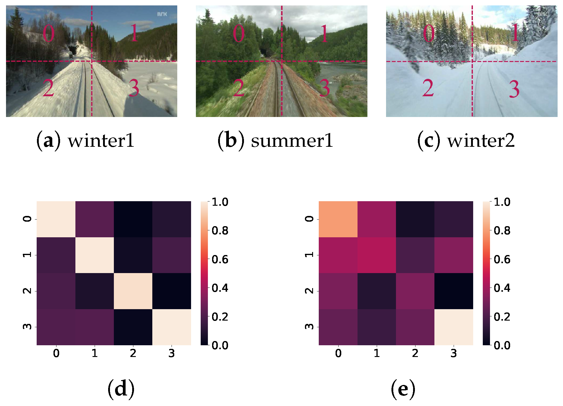
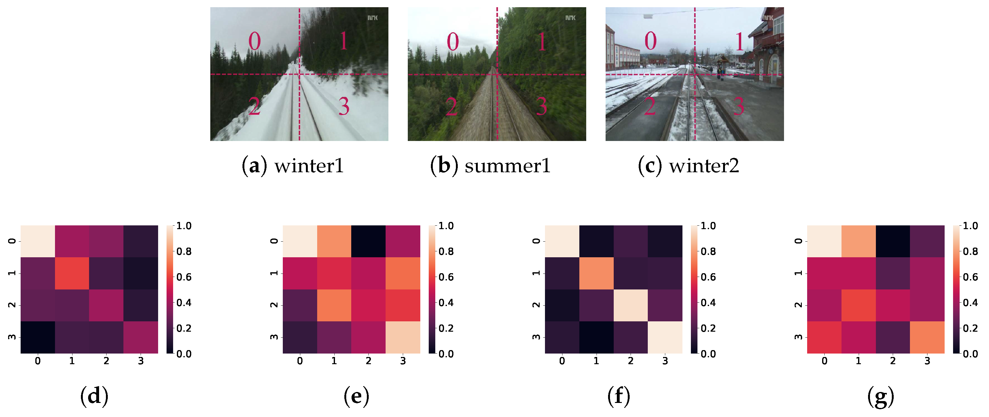
4.1. Datasets

To evaluate the performance of the proposed system in response to the appearance-changing conditions for LCD, we chose three widely used datasets as the test set (i.e., Gardens Point [50], Nordland [51], and St. Lucia [52] datasets). The details of these three datasets are shown in

Table 2. Description of the Testing Loop Closure Detection Datasets with Changing Environmental Conditions.

Dataset	Image Resolution & Frequency	Image Type	Environment	Appearance Variation	Viewpoint Variation
Gardens Point [50]	1920 × 1080, 30 Hz	RGB	Campus	Day-Night	Moderate
Nordland [51]	1920 × 1080, 25 Hz	RGB	Train journey	Winter-Summer	Small
St. Lucia [52]	640 × 480, 15 Hz	RGB	Suburban	Morning-Afternoon	Moderate

, and the appearance variations of some examples are shown in Figure 6.

The details of the datasets are as follows:

Gardens Point dataset is collected on the campus of Queensland University of Technology while crossing the walkways during the day (along both sides) and at night (along the right side only). The day-right and night-right pairs are adopted as DAY and NIGHT to test the performance under significant illumination variation. The ground truth is created manually according to the location.

Nordland dataset is produced from a TV documentary that chronicles a train journey covering the changing appearance of four seasons. After arranging images from different seasons following their positions, the ground truth can be constructed based on image indexes. Images taken in winter and summer (denoted as WINTER and SUMMER) that contain significant variations in appearance are selected as part of the test set.

St. Lucia dataset is captured in the suburbs at five different times (8:45, 10:00, 12:10, 14:10, and 15:45), with significant appearance changes due to the illumination changes. The ground truth is obtained from GPS logs. For the intense contrasts, SL0845 and SL1410 (collected at 8:45 and 14:10) are selected to form the test set.

4.2. Evaluation Metrics

Evaluation techniques typically focus on precision-recall metrics [53]. Precision is defined as the ratio of accurate matches (i.e., true positives (TP)) to the total system detections (i.e., true positives plus false positives (FP)). Recall denotes the ratio of true positives to the total ground truth (i.e., the sum of true positives and false negatives (FN)). They can be defined as follows:

$$Precision={\displaystyle \frac{TP}{TP+FP}}$$

(17)

$$Recall={\displaystyle \frac{TP}{TP+FN}}$$

(18)

Based on this, we adopt the Precision-Recall (PR) curve to evaluate the relationship between these metrics. The curve closer to the top right has better performance.

In addition, two other evaluation metrics are also adopted here: (1) the mean average precision (mAP), which refers to the coverage area under the PR curve as:

$$AP={\int }_0^{1}P\left(r\right)\mathrm{d}r$$

(19)

where $P\left(r\right)$ represents the PR curve and r is the recall. (2) the maximum recall rate at 100% precision. Note that the size of the area under the PR curve is positively correlated with the effectiveness of the LCD methods.

4.3. Experimental Results

4.3.1. Qualitative and Quantitative Comparisons

In this experiment, comparisons are made on the Gardens Point, Nordland, and St. Lucia datasets. To comprehensively measure the effectiveness of MetricNet, we select multiple typical and representative approaches from different perspectives for comparison, such as the methods based on learned feature representations (Place-ResNet [23], NetVLAD [24], CAE-VLAD-Net [25]), sequence-to-sequence methods (SeqSLAM [5], MCN [31], SMCN [32]), methods designed for appearance variations (SAES [35], CALC2.0 [36], Schubert et al. [37]), and viewpoint changes (Jin et al. [42]).

To test SAES, we use the model trained on the SPED_900 dataset by the authors. The CALC2.0 is trained on the COCO dataset [54], and the implementation used for the experiments is the same as described in their paper. As for Place-ResNet, the pre-trained models are utilized to make the comparison. The MATLAB source of NetVLAD is available from [24] along with several sets of weights. The results of SeqSLAM [5], MCN [31], SMCN [32], CAE-VLAD-Net [25], Jin et al. [42], and Schubert et al. [37] presented in this section are obtained from their published studies. For a fair comparison, the versions of the models chosen for the experiments are relevant to the methodology in our paper and largely follow the settings in their published papers.

We evaluate the model’s effectiveness from multiple perspectives. Firstly, the PR curve results of the methods designed for appearance variations are compared. The PR curves are drawn based on the experimental results, as shown in Figure 7. It can be seen that, as the similarity threshold increases, all the recall rates show a slow downward trend when the precision is high. MetricNet achieves the most promising performance due to its PR curve closer to the upper right corner. It demonstrates that MetricNet has a relatively prominent generalization ability in dealing with the test set with significant appearance variations.

Compared to SAES, the backbone of our method, the improvements of MetricNet are mainly due to the utilization of channel-wise attention distillation and adaptively weighted similarity scores. Although our method achieves slightly lower precision as the recall rate increases up to a certain threshold on the Gardens Point and St. Lucia datasets, MetricNet is more advantageous in terms of the area under the PR-curve. It is noteworthy that our method performs best on the Nordland dataset compared to the experimental results on other datasets, highlighting the robustness of MetricNet to seasonal variations. We attribute this to the fact that the images in the dataset were taken along a fixed train track, which minimizes changes in viewpoint. Illumination variations have long posed a challenge in visual tasks. While our method exhibits some sensitivity to illumination variations in the St. Lucia dataset, it achieves the best performance overall.

The corresponding results of the maximum recall rate at 100% precision are shown in Figure 8. It can be seen that MetricNet can achieve the highest recall rate at 100% precision, reaching 43.97%, 44.49%, and 26.71% on the three datasets, respectively. Compared to the other approaches, MetricNet improves performance by up to 10–30%, implying the robustness of MetricNet in reducing false positives for true loop closures. We conclude that improving the discrimination between positive and negative samples in the Similarity Measurement Module is helpful under such conditions.

To quantitatively verify the performance of MetricNet and other competitive SOTA algorithms, we compare their mean average precision (area under the PR curve), as shown in

Table 3. The mAP Comparison of Different Networks.

Algorithm	Dataset
	Gardens Point	Nordland	St. Lucia
SAES [35]	0.6997	0.7162	0.7098
CALC2.0 [36]	0.7284	0.6348	0.5869
Schubert et al. [37]	0.6900	0.7500	0.6800
Place-ResNet [23]	0.3048	0.8209	0.6860
NetVLAD [24]	0.7433	0.5320	0.5660
SeqSLAM [5]	0.4300	0.7233	0.2267
MCN [31]	0.7400	0.8211	0.6241
SMCN [32]	0.6500	0.5300	-
CAE-VLAD-Net [25]	0.8400	0.7500	-
Jin et al. [42]	0.8380	0.7280	-
Pairwise	0.5320	0.6843	0.5781
MetricNet_$\omega$	0.7289	0.6389	0.6920
MetricNet_$\alpha$	0.7793	0.8173	0.7422
MetricNet	0.7831	0.8458	0.7476

- means that the corresponding method did not experiment on the open dataset. The best performance is in bold and the second best is underlined.

. Compared to the most related method, SAES, MetricNet outperforms it by up to 11.92%, 18.10%, and 5.33% on the Gardens Point, Nordland, and St. Lucia datasets, respectively. This demonstrates that our feature refinement and weighted similarity modules can significantly enhance the accuracy of LCD. It also shows that MetricNet and SAES achieve the two best results on St. Lucia, which verifies the robustness of the patch-based LCD architecture.

As for the other two models designed for changing environments, CALC2.0 [36] and Schubert et al. [37] obtain reliable results by using different technical solutions. By taking semantic and geometric information into account, CALC2.0 is able to perform well under changing lighting conditions. Schubert et al.’s work also proves the importance of clustering and PCA-based descriptor standardization. However, MetricNet yields more promising and stable results. It can be seen that our method performs well without the addition of extra perceptual information. Additionally, incorporating similarity measurement inspired by metric learning can further enhance the strengths of the proposed method.

Although the SOTA methods based on sequence-to-sequence matching, i.e., SeqSLAM [5], MCN [31], and SMCN [32], produce promising average precision by exploiting the sequential characteristic of robotic data streams, their results are inferior to those of MetricNet when it comes to long-term operation with significant appearance variations. The results of Place-ResNet [23], NetVLAD [24], and CAE-VLAD-Net [25] demonstrate their robustness to environmental changes to some extent. The learned feature representation of CAE-VLAD-Net is more effective than the simple CNN-based network used in our method. We conclude this is mainly because of the combination of convolutional neural networks and stacked auto-encoders. Jin et al. [42] propose the multi-tuplet clusters loss function together with a mini-batch construction scheme, which shows advantages when dealing with changing illumination. Nevertheless, our approach yields much better performance on seasonal changes in Nordland.

We further conduct an ablation experiment to evaluate the effectiveness of the self-adaptive parameters. Note that the Pairwise baseline is achieved by a cosine similarity-based comparison using deep image descriptors computed by AlexNet. MetricNet_$\omega$ is the ablation model with ${\omega }_i$ = 1/4. MetricNet_$\alpha$ is the version with the constant parameter $\alpha$ calculated by:

$$\alpha ={\displaystyle \frac{1}{1+e^d}}$$

(20)

where d is calculated by Equation (9). It can be seen that MetricNet delivers the best estimation on the Nordland and St. Lucia datasets and the third-best one on Gardens Point. When compared to MetricNet_$\omega$, the results of MetricNet_$\alpha$ are much closer to those of MetricNet. They both yield lower average precision than MetricNet. This demonstrates that the parameters $\omega$ and $\alpha$ both have a significant impact on loop closure detection, and different ${\omega }_i$ for each $M_{ii}$ makes the method more robust in distinguishing positive and negative pairs. Besides, compared with Pairwise, MetricNet achieves better average precision of up to 47.20%, 23.60%, and 29.3% on Gardens Point, Nordland, and St. Lucia datasets, respectively.

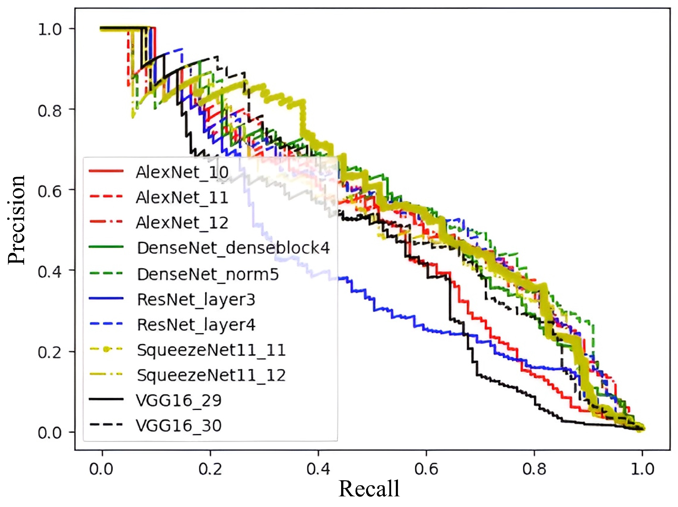
4.3.2. Evaluation of Feature Extraction Component

To evaluate the performance of the feature extraction module, we present an ablation study comparing MetricNet with the closely related patch-matching-based method like [35]. The approach [35] directly divides each input image into four patches for further deep feature extraction. In this experiment, we named this ablation version as MetricNet_direct.

The experimental results on the Nordland dataset are shown in Figure 9. The frames of winter1 (Figure 9a) and summer1 (Figure 9b) are collected at the same place, while winter2 in Figure 9c is captured from a different location. The similarity matrices of winter1 and summer1 calculated by MetricNet_direct and MetricNet are shown in Figure 9d and Figure 9f, respectively. The similarity matrices of winter2 and summer1 calculated by MetricNet_direct and MetricNet are shown in Figure 9e and Figure 9g, respectively.

It can be seen that our feature refinement in the Channel Weighting Module significantly improves the performance of MetricNet. It can help the proposed method construct a more robust similarity matrix for subsequent similarity score calculation. This superior similarity matrix naturally provides a more stable classification basis for the similarity measurement. Although both MetricNet_direct and MetricNet achieve promising performance, MetricNet enlarges the difference between positive and negative pairs. When encountering positive pairs, the diagonal values of MetricNet are much larger than the off-diagonal ones. For the negative pairs, the values of the similarity matrix tend to be more random. We can conclude that the MetricNet algorithm has the ability to make the difference between positive and negative more prominent, making the inputs easier to distinguish.

To demonstrate this conclusion more clearly, we compare the differences between the mean of diagonal and off-diagonal values (calculated by Equation (9)) in the positive-pair and negative-pair similarity matrices. The differences d generated by MetricNet and MetricNet_direct can be defined as $d_1$ and $d_2$, respectively. We plot the probability density distribution of $\Delta$ = $d_1-d_2$ for positive and negative pairs on each dataset. As shown in Figure 10, the horizontal axis represents the similarity difference of $\Delta$, and the vertical axis represents the corresponding probability density. The corresponding probability density function can be expressed as:

$$f(\Delta )={\displaystyle \frac{1}{\sqrt{2\pi {\sigma }^2}}}{e}^{-\frac{{(\Delta -\mu )}^2}{2{\sigma }^2}}$$

(21)

where $\mu$ and $\sigma$ denote the mean and standard deviation of $\Delta$, respectively.

The area under the curve represents the probability of $\Delta$. When $\Delta$ > 0, we fill the area under the curve with orange, otherwise with medium violet red. As shown in Figure 10, testing on the positive pairs from three datasets, the similarity differences obtained by MetricNet are mostly more significant than those obtained by MetricNet_direct. It means that MetricNet’s weighted similarity matrix can make the image descriptors more distinguishable. Besides, as for the negative pairs, MetricNet tends to generate the similarity matrix with more random diagonal and off-diagonal values, where the difference between these elements is evidently smaller.

All the comparisons can demonstrate that the utilization of attention-based channel weighting and the similarity matrix weighted by relative value relation can help improve the discriminability of descriptors for positive pairs and reduce the differences of values in the similarity matrix for negative pairs. Moreover, the visual information at the boundaries of each patch is integral for feature extraction. Using overlapping convolution kernels in convolutional neural networks to retain contextual information at the boundaries of feature blocks is more effective than directly segmenting the original image.

4.3.3. Evaluation of Similarity Measurement Component

In this section, another ablation study is conducted to evaluate the proposed similarity measurement component. We utilized three conventional distance metrics, i.e., cosine, Euclidean, and average similarity (AVE-SIMI) distance, to replace the adaptive weighted similarity matrix in MetricNet. In this experiment, the cosine and Euclidean distances are computed directly to obtain the similarity matrix based on the complete image features without dividing them into patches. As for the version with AVE-SIMI, all the similarity matrix elements are directly averaged for the final measurement.

The PR curves tested on three datasets (i.e., Gardens Point, Nordland, and St. Lucia datasets) are shown in Figure 11. It can be observed that both MetricNet and the ablation models can provide promising precision at low recall rates. However, MetricNet performs better when the recall rate is high. It can be concluded that MetricNet can correctly detect more true loops than other versions, which reveals the effectiveness of the proposed similarity measurement. We conclude that this is mainly because the similarity between images is reflected in the absolute distance and direction between the feature descriptors, and the lack of spatial information in the features is compensated by the construction of the similarity matrix based on adaptive weighting in MetricNet.

Figure 12 shows their maximum recall rate at the precision of 100%. Testing on all the datasets, MetricNet obtains the highest recall rate at 100% precision, and the method based on Euclidean distance gets the worst performance. The experimental results reveal that MetricNet can yield fewer false loop detections.

The mean average precision of MetricNet and the ablation methods is shown in

Table 4. The mAP Comparison of Different Measurement Methods.

Dataset	Algorithm
	Euclidean	Cosine	AVE-SIMI	MetricNet
Gardens Point	0.4932	0.5663	0.5805	0.7831
Nordland	0.4638	0.4885	0.4736	0.8458
St. Lucia	0.3828	0.5205	0.5659	0.7476

The best performance is in bold and the second best is underlined.

and Figure 13. It can be seen that the proposed method achieves the best mAP performance on all three datasets, which indicates the considerable reliability of MetricNet in handling scenes with significant appearance variations.

The above comparisons emphasize the meaningfulness of optimizing the similarity measurement of LCD networks. After comparing the Euclidean and cosine-based methods, it can be found that the full utilization of the image information to construct a similarity matrix will partially solve the lack of sufficient global spatial cues from the feature extraction. Meanwhile, after using the adaptive weighting mechanism, MetricNet enhances the difference between positive and negative pair similarity. MetricNet can fully consider the contributions of various features to the overall similarity calculation, which can be reflected in the comparisons with AVE-SIMI.

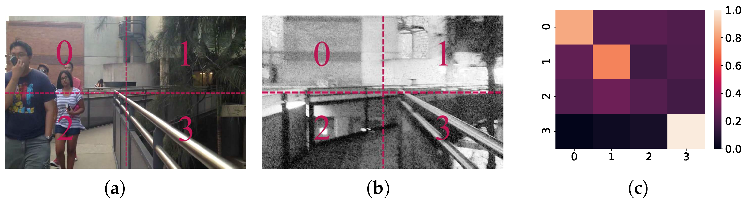
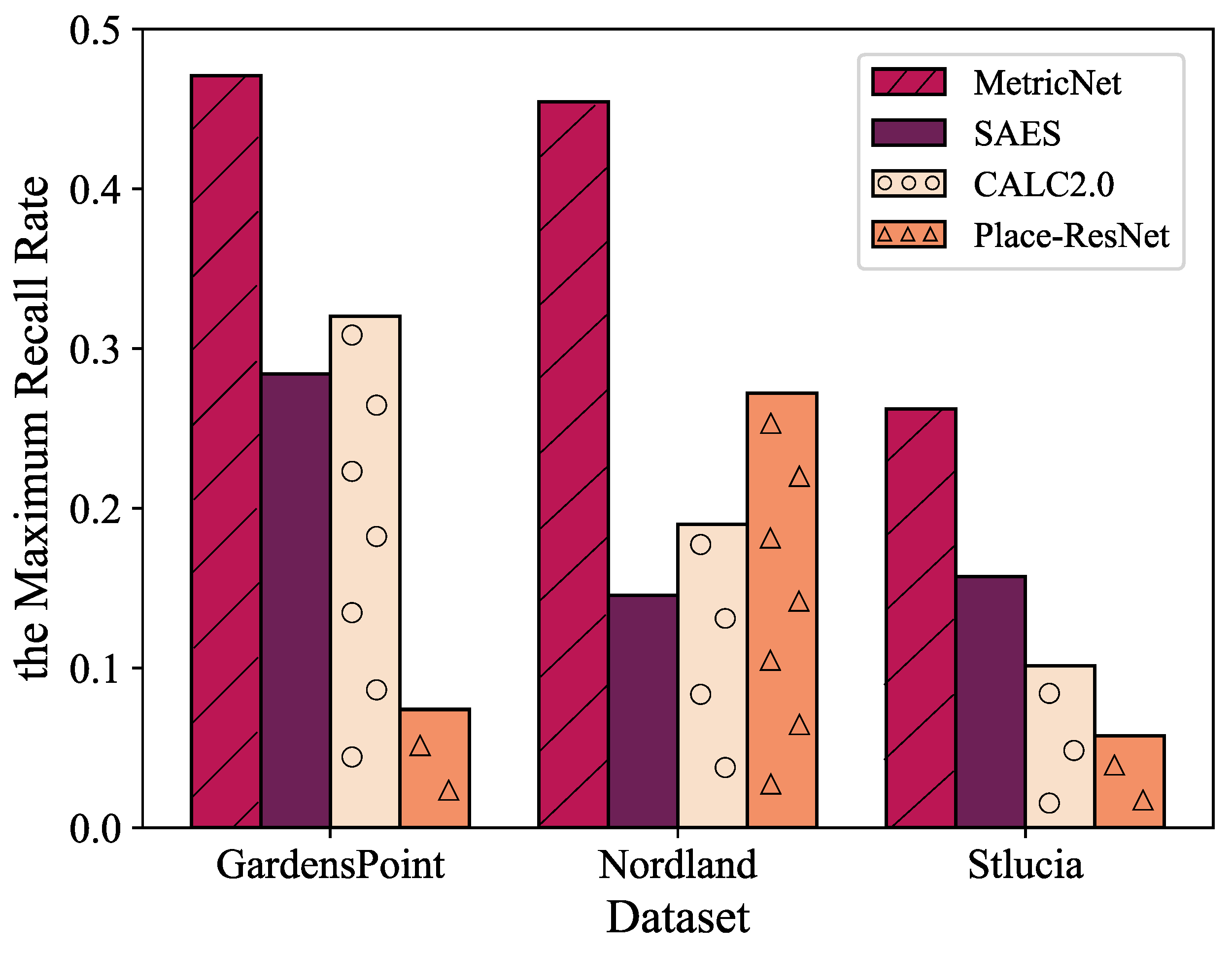
4.3.4. Results for Distinct Viewpoint Variations

Although MetricNet is an LCD model designed to handle test scenes with significant appearance variations, we also introduce another two open datasets (Oxford5K [55] and Paris6K [56]) to verify the effectiveness of the proposed method. Oxford5K is a dataset containing 5062 images of buildings from 11 landmarks in Oxford. Each landmark has 5 query instances, and 55 query groups are generated. Besides, Paris6K contains 6412 images of Paris landmarks, which are classified into 12 categories. Both of them have significant variations in viewpoint and appearance, as shown in Figure 14.

The images in these two datasets are not collected sequentially, and they are usually used for image retrieval rather than localization tasks. Therefore, the sequence-based LCD algorithms cannot work in this condition. Since it is unfair to adopt state-of-the-art algorithms specifically designed for viewpoint variations, we compare the proposed method with related works, such as CBE [13], SGH [14], ITQ [12], LPM [18], UBEF [15], and SMVF-CVT [19], as shown in

Table 5. The mAP Comparison of Different Networks.

Algorithm	Dataset
	Oxford5K	Paris6K
CBE [13]	0.5829	0.6989
SGH [14]	0.4726	0.5647
ITQ [12]	0.6006	0.5980
LPM [18]	0.6065	-
UBEF [15]	0.6249	0.6642
SMVF-CVT [19]	0.6514	0.7281
Proposed methods
MetricNet	0.5908	0.5732
MetricNet_3×3	0.6007	0.5767

- means that the corresponding method did not experiment on the open dataset. The best performance is in bold, and the second best is underlined.

.

Note that all the binary encoding-based algorithms (i.e., CBE, SGH, ITQ, and UBEF) utilize CNN-based image descriptors as features. SMVF-CVT simultaneously uses multi-view features, such as CNN, VLAD+, and TEDA. We also include another ablation model, MetricNet_3×3 (i.e., the version with the same backbone as MetricNet but have the feature maps divided into $3\times 3$ patches), to handle this more challenging situation. MetricNet_3×3 has a smaller particle size when processing feature maps for similarity matrix construction.

Despite the viewpoint variations of the Oxford5K and Paris6K datasets being significantly dramatic, the proposed methods still achieve reliable performance compared to the other algorithms. The results of SMVF-CVT demonstrate that utilizing multi-view fusion features can help improve image matching performance, which is designed for instance-level image retrieval. It can also be seen that MetricNet_3×3 is more effective in dealing with the testing datasets having significant viewpoint variations. It gets slightly higher mean average precision than the original version on the Oxford5K and Paris6K datasets. We attribute this to the version that splits images into more patches, enabling the network to focus on relations between more refined feature sub-regions, thereby enhancing the model’s robustness to significant viewpoint variations.

Although our network is able to produce relatively reliable detection results to some extent, it is still not comparable to professional methods for image retrieval tasks. We believe this limitation arises because the algorithm relies solely on a single image without considering additional perceptual information like semantics, which limits the validity of the proposed method facing viewpoint variations. Moreover, the patch-to-patch design of MetricNet is not adequate for the task of filtering and selecting the most relevant regions.

4.3.5. Application of Loop Closure Detection

To validate the practical effectiveness of the proposed method in the vSLAM localization problem, we integrate MetricNet with a localization method and use its estimations to optimize the VO’s prediction. To ensure the reasonableness of this experiment, we only perform the optimization by adding loop closure constraints to trajectories where MetricNet predicts the existence of closed loops. For this experiment, we use one of the most influential outdoor VO/SLAM benchmarks, KITTI [57], as the experimental dataset. Following the commonly used train/test split in deep VOs, we adopt Sequence 00, 02, 08, and 09 of the KITTI dataset to fine-tune the MetricNet and utilize Sequence 05 and 06 to perform the evaluation. ContextAVO [58] is adopted as the visual front-end, with pose graph optimization implemented in g2o [59] as the back-end.

The visualization results are illustrated in Figure 15. It can be seen that the trajectories optimized based on associations from loop closure detection effectively reduce the cumulative error and drift. Despite some inconsistent information changes between query and matched images, i.e., dynamic objects and occlusions, the prediction of MetricNet remains promising. This suggests that MetricNet is able to provide correct and effective associations for place recognition in localization applications.

4.3.6. Computational Performance

The average computational cost of two proposed methods (i.e., MetricNet and MetricNet_3×3) and SAES [35] is compared in the following experiments. We test the computational cost of all module processes: (1) the feature extraction process of the neural networks, (2) the construction of the similarity matrices, and (3) the similarity calculation between image pairs. The Nordland dataset is utilized here because of its relatively long length. An Intel Xeon CPU E5-2678 v3 (2.50 GHz) and an NVIDIA GeForce Titan XP GPU are used here.

As shown in

Table 6. Computational Performances on the Nordland Dataset.

Algorithm	Processing Time(s)
	Feature Extraction	Similarity Matrix Construction	Similarity Calculation
SAES [35]	0.0218	0.0065	0.0025
MetricNet	0.0282	0.0045	0.0020
MetricNet_3×3	0.0282	0.0047	0.0021

, the feature extraction component takes more execution time than the other two processes. This is mainly because of the large number of computations in deep neural networks. Besides, due to the calculation of channel weighting, our methods take more time in feature extraction.

Compared with SAES, the two proposed methods greatly reduce the computational cost of constructing the similarity matrix and calculating the similarity score. Moreover, MetricNet outperforms MetricNet_3×3 by up to 4.4% and 5.0% in these two processes, respectively. Though the effects of both proposed methods are considerable, MetricNet proved to be more robust in terms of efficiency. Note that the parameters and GFLOPs of MetricNet are 2.47 M and 1.03 G, respectively.

In loop closure detection, it is significant to calculate the similarity score in real-time. With the increasing number of previous images in the database, the computational cost of pairwise image matching will gradually increase. Therefore, we further test the algorithms’ computational performance when the frame index rises. As shown in Figure 16, as the number of previous images in the database grows, MetricNet achieves higher efficiency and better real-time performance.

5. Conclusions

This paper proposes a novel LCD framework, MetricNet, for dramatic appearance variations, such as illumination, seasonal changes, and dynamic interference. In the proposed method, feature extraction and similarity measurement components are trained and deployed in an end-to-end manner. It takes the current and previous image pairs as input and extracts the high-dimensional visual features utilizing the AlexNet-based feature extraction network. The self-attention component Channel Weighting Module is designed to refine the image descriptors to preserve discriminative cues. Then the promising similarity score is adaptively weighted in the Similarity Measurement Module based on the feature relationship of the patch-by-patch similarity matrix, which helps to further improve the detection performance. Extensive experiments on various datasets validate the appealing precision, generalization ability, and dependability of MetricNet in scenes with significant appearance and even viewpoint variations. Compared to many state-of-the-art learning-based methods, MetricNet’s average accuracy has increased by 7.51%, 3.03%, and 5.33%, respectively.

Although our model has achieved feasible results in LCD, there are still shortcomings of MetricNet in dealing with sequential input and image retrieval problems with significant viewpoint variations. In addition, MetricNet currently only applies to images of fixed size. Images of different sizes need to be cropped or resized before entering the network, which may result in incomplete image information compared to the original, leading to poor loop closure accuracy. In the future, we will further optimize the proposed method by jointly considering semantic, appearance, and geometric information. After utilizing this environmental understanding information, LCD methods will provide a higher degree of invariance to environmental changes.To solve the problem of fixed-size input, we intend to introduce spatial pyramid pooling (SPP) and various feature fusion methods to improve input adaptability and image feature representation capabilities. Furthermore, to achieve long-term operation in LCD, incremental learning technologies will be investigated in our future network.

References

1. Fuentes-Pacheco, J.; Ruiz-Ascencio, J.; Rendón-Mancha, J.M. Visual simultaneous localization and mapping: A survey. Artif. Intell. Rev. 2015, 43, 55–81. [Google Scholar] [CrossRef]
2. Mur-Artal, R.; Tardós, J.D. Orb-slam2: An open-source slam system for monocular, stereo, and rgb-d cameras. IEEE Trans. Robot. 2017, 33, 1255–1262. [Google Scholar] [CrossRef]
3. Labbe, M.; Michaud, F. Appearance-based loop closure detection for online large-scale and long-term operation. IEEE Trans. Robot. 2013, 29, 734–745. [Google Scholar] [CrossRef]
4. Csurka, G.; Dance, C.; Fan, L.; Willamowski, J.; Bray, C. Visual categorization with bags of keypoints. In Proceedings of the Workshop on Statistical Learning in Computer Vision, ECCV, Prague, Czech Republic, 11–14 May 2004; Volume 1, pp. 1–2. [Google Scholar]
5. Milford, M.J.; Wyeth, G.F. SeqSLAM: Visual route-based navigation for sunny summer days and stormy winter nights. In Proceedings of the 2012 IEEE International Conference on Robotics and Automation, St. Paul, MN, USA, 14–18 May 2012; pp. 1643–1649. [Google Scholar]
6. Hou, Y.; Zhang, H.; Zhou, S. Convolutional neural network-based image representation for visual loop closure detection. In Proceedings of the 2015 IEEE International Conference on Information and Automation, Lijiang, China, 8–10 August 2015; pp. 2238–2245. [Google Scholar]
7. Calonder, M.; Lepetit, V.; Strecha, C.; Fua, P. Brief: Binary robust independent elementary features. In Proceedings of the European Conference on Computer Vision, Heraklion, Greece, 5–11 September 2010; Springer: Berlin/Heidelberg, Germany, 2010; pp. 778–792. [Google Scholar]
8. Bay, H.; Tuytelaars, T.; Van Gool, L. Surf: Speeded up robust features. In Proceedings of the European Conference on Computer Vision, Graz, Austria, 7–13 May 2006; Springer: Berlin/Heidelberg, Germany, 2006; pp. 404–417. [Google Scholar]
9. Siam, S.M.; Zhang, H. Fast-SeqSLAM: A fast appearance based place recognition algorithm. In Proceedings of the 2017 IEEE International Conference on Robotics and Automation (ICRA), Singapore, 29 May–3 June 2017; pp. 5702–5708. [Google Scholar]
10. Cummins, M.; Newman, P. FAB-MAP: Probabilistic localization and mapping in the space of appearance. Int. J. Robot. Res. 2008, 27, 647–665. [Google Scholar] [CrossRef]
11. Jégou, H.; Douze, M.; Schmid, C.; Pérez, P. Aggregating local descriptors into a compact image representation. In Proceedings of the 2010 IEEE Computer Society Conference on Computer Vision and Pattern Recognition, San Francisco, CA, USA, 13–18 June 2010; pp. 3304–3311. [Google Scholar]
12. Gong, Y.; Lazebnik, S.; Gordo, A.; Perronnin, F. Iterative quantization: A procrustean approach to learning binary codes for large-scale image retrieval. IEEE Trans. Pattern Anal. Mach. Intell. 2012, 35, 2916–2929. [Google Scholar] [CrossRef] [PubMed]
13. Yu, F.; Kumar, S.; Gong, Y.; Chang, S.F. Circulant binary embedding. In Proceedings of the International Conference on Machine Learning, PMLR, Beijing, China, 22–24 June 2014; pp. 946–954. [Google Scholar]
14. Jiang, Q.Y.; Li, W.J. Scalable graph hashing with feature transformation. In Proceedings of the Twenty-Fourth International Joint Conference on Artificial Intelligence, Buenos Aires, Argentina, 25–31 July 2015. [Google Scholar]
15. He, Y.; Chen, Y. A Unified Binary Embedding Framework for Image Retrieval. In Proceedings of the 2021 International Joint Conference on Neural Networks (IJCNN), Shenzhen, China, 18–22 July 2021; pp. 1–7. [Google Scholar]
16. Lowe, D.G. Distinctive image features from scale-invariant keypoints. Int. J. Comput. Vis. 2004, 60, 91–110. [Google Scholar] [CrossRef]
17. Rublee, E.; Rabaud, V.; Konolige, K.; Bradski, G. ORB: An efficient alternative to SIFT or SURF. In Proceedings of the 2011 International Conference on Computer Vision, Barcelona, Spain, 6–13 November 2011; pp. 2564–2571. [Google Scholar]
18. Ma, J.; Zhao, J.; Jiang, J.; Zhou, H.; Guo, X. Locality preserving matching. Int. J. Comput. Vis. 2019, 127, 512–531. [Google Scholar] [CrossRef]
19. Li, J.; Yang, B.; Yang, W.; Sun, C.; Xu, J. Subspace-based multi-view fusion for instance-level image retrieval. Vis. Comput. 2021, 37, 619–633. [Google Scholar] [CrossRef]
20. Krizhevsky, A.; Sutskever, I.; Hinton, G.E. Imagenet classification with deep convolutional neural networks. Adv. Neural Inf. Process. Syst. 2012, 25, 1–9. [Google Scholar] [CrossRef]
21. Simonyan, K.; Zisserman, A. Very deep convolutional networks for large-scale image recognition. arXiv 2014, arXiv:1409.1556. [Google Scholar]
22. He, K.; Zhang, X.; Ren, S.; Sun, J. Deep residual learning for image recognition. In Proceedings of the IEEE Conference on Computer Vision and Pattern Recognition, Las Vegas, NV, USA, 27–30 June 2016; pp. 770–778. [Google Scholar]
23. Zhou, B.; Lapedriza, A.; Khosla, A.; Oliva, A.; Torralba, A. Places: A 10 million image database for scene recognition. IEEE Trans. Pattern Anal. Mach. Intell. 2017, 40, 1452–1464. [Google Scholar] [CrossRef]
24. Arandjelovic, R.; Gronat, P.; Torii, A.; Pajdla, T.; Sivic, J. NetVLAD: CNN Architecture for Weakly Supervised Place Recognition. In Proceedings of the IEEE Conference on Computer Vision and Pattern Recognition, Las Vegas, NV, USA, 27–30 June 2016; pp. 5297–5307. [Google Scholar]
25. Liu, Y.; Li, Y.; Zhang, H.; Xiong, N. CAE-VLAD-Net: A Loop Closure Detection System for Mobile Robots Using Convolutional Auto-Encoders Network with VLAD. 2023. Available online: https://www.researchsquare.com/article/rs-2601576/v1 (accessed on 3 June 2024).
26. An, S.; Zhu, H.; Wei, D.; Tsintotas, K.A.; Gasteratos, A. Fast and incremental loop closure detection with deep features and proximity graphs. J. Field Robot. 2022, 39, 473–493. [Google Scholar] [CrossRef]
27. Yu, G.; Li, H.; Wang, Y.; Chen, P.; Zhou, B. A review on cooperative perception and control supported infrastructure-vehicle system. Green Energy Intell. Transp. 2022, 1, 100023. [Google Scholar] [CrossRef]
28. Benbihi, A.; Arravechia, S.; Geist, M.; Pradalier, C. Image-based place recognition on bucolic environment across seasons from semantic edge description. In Proceedings of the 2020 IEEE International Conference on Robotics and Automation (ICRA), Paris, France, 31 May–31 August 2020; pp. 3032–3038. [Google Scholar]
29. Chen, Z.; Maffra, F.; Sa, I.; Chli, M. Only look once, mining distinctive landmarks from convnet for visual place recognition. In Proceedings of the 2017 IEEE/RSJ International Conference on Intelligent Robots and Systems (IROS), Vancouver, BC, Canada, 24–28 September 2017; pp. 9–16. [Google Scholar]
30. Lu, F.; Chen, B.; Zhou, X.D.; Song, D. STA-VPR: Spatio-temporal alignment for visual place recognition. IEEE Robot. Autom. Lett. 2021, 6, 4297–4304. [Google Scholar] [CrossRef]
31. Neubert, P.; Schubert, S.; Protzel, P. A neurologically inspired sequence processing model for mobile robot place recognition. IEEE Robot. Autom. Lett. 2019, 4, 3200–3207. [Google Scholar] [CrossRef]
32. Huang, G.; Chen, A.; Gao, H.; Yang, P. SMCN: Simplified mini-column network for visual place recognition. J. Phys. Conf. Ser. 2021, 2024, 012032. [Google Scholar] [CrossRef]
33. Liu, Y.; Xiang, R.; Zhang, Q.; Ren, Z.; Cheng, J. Loop closure detection based on improved hybrid deep learning architecture. In Proceedings of the 2019 IEEE International Conferences on Ubiquitous Computing & Communications (IUCC) and Data Science and Computational Intelligence (DSCI) and Smart Computing, Networking and Services (SmartCNS), Shenyang, China, 21–23 October 2019; pp. 312–317. [Google Scholar]
34. Chen, B.; Yuan, D.; Liu, C.; Wu, Q. Loop closure detection based on multi-scale deep feature fusion. Appl. Sci. 2019, 9, 1120. [Google Scholar] [CrossRef]
35. Zhao, C.; Ding, R.; Key, H.L. End-To-End Visual Place Recognition Based on Deep Metric Learning and Self-Adaptively Enhanced Similarity Metric. In Proceedings of the 2019 IEEE International Conference on Image Processing (ICIP), Taipei, Taiwan, 22–25 September 2019; pp. 275–279. [Google Scholar]
36. Merrill, N.; Huang, G. CALC2.0: Combining appearance, semantic and geometric information for robust and efficient visual loop closure. In Proceedings of the 2019 IEEE/RSJ International Conference on Intelligent Robots and Systems (IROS), Venetian Macao, Macau, 3–8 November 2019; pp. 4554–4561. [Google Scholar]
37. Schubert, S.; Neubert, P.; Protzel, P. Unsupervised learning methods for visual place recognition in discretely and continuously changing environments. In Proceedings of the 2020 IEEE International Conference on Robotics and Automation (ICRA), Paris, France, 31 May–31 August 2020; pp. 4372–4378. [Google Scholar]
38. Osman, H.; Darwish, N.; Bayoumi, A. PlaceNet: A multi-scale semantic-aware model for visual loop closure detection. Eng. Appl. Artif. Intell. 2023, 119, 105797. [Google Scholar] [CrossRef]
39. Arshad, S.; Kim, G.W. Role of deep learning in loop closure detection for visual and lidar slam: A survey. Sensors 2021, 21, 1243. [Google Scholar] [CrossRef]
40. Gao, X.; Zhang, T. Unsupervised learning to detect loops using deep neural networks for visual SLAM system. Auton. Robot. 2017, 41, 1–18. [Google Scholar] [CrossRef]
41. Balaska, V.; Bampis, L.; Kansizoglou, I.; Gasteratos, A. Enhancing satellite semantic maps with ground-level imagery. Robot. Auton. Syst. 2021, 139, 103760. [Google Scholar] [CrossRef]
42. Jin, S.; Gao, Y.; Chen, L. Improved deep distance learning for visual loop closure detection in smart city. Peer-to-Peer Netw. Appl. 2020, 13, 1260–1271. [Google Scholar] [CrossRef]
43. Garg, S.; Suenderhauf, N.; Milford, M. Semantic–geometric visual place recognition: A new perspective for reconciling opposing views. Int. J. Robot. Res. 2022, 41, 573–598. [Google Scholar] [CrossRef]
44. Yu, C.; Liu, Z.; Liu, X.J.; Qiao, F.; Wang, Y.; Xie, F.; Wei, Q.; Yang, Y. A DenseNet feature-based loop closure method for visual SLAM system. In Proceedings of the 2019 IEEE International Conference on Robotics and Biomimetics (ROBIO), Dali, China, 6–8 December 2019; pp. 258–265. [Google Scholar]
45. Kulis, B. Metric learning: A survey. Found. Trends® Mach. Learn. 2013, 5, 287–364. [Google Scholar] [CrossRef]
46. Chen, Z.; Jacobson, A.; Sünderhauf, N.; Upcroft, B.; Liu, L.; Shen, C.; Reid, I.; Milford, M. Deep learning features at scale for visual place recognition. In Proceedings of the 2017 IEEE International Conference on Robotics and Automation (ICRA), Singapore, 29 May–3 June 2017; pp. 3223–3230. [Google Scholar]
47. Paszke, A.; Gross, S.; Massa, F.; Lerer, A.; Bradbury, J.; Chanan, G.; Killeen, T.; Lin, Z.; Gimelshein, N.; Antiga, L.; et al. Pytorch: An imperative style, high-performance deep learning library. Adv. Neural Inf. Process. Syst. 2019, 32, 1–12. [Google Scholar]
48. Deng, J.; Dong, W.; Socher, R.; Li, L.J.; Li, K.; Fei-Fei, L. Imagenet: A large-scale hierarchical image database. In Proceedings of the 2009 IEEE Conference on Computer Vision and Pattern Recognition, Miami, FL, USA, 20–25 June 2009; pp. 248–255. [Google Scholar]
49. Kingma, D.P.; Ba, J. Adam: A method for stochastic optimization. arXiv 2014, arXiv:1412.6980. [Google Scholar]
50. Glover, A. Day and night, left and right. Zenodo, 2014; 10. [Google Scholar] [CrossRef]
51. Sünderhauf, N.; Neubert, P.; Protzel, P. Are we there yet? Challenging SeqSLAM on a 3000 km journey across all four seasons. In Proceedings of the Workshop on Long-Term Autonomy, IEEE International Conference on Robotics and Automation (ICRA), Karlsruhe, Germany, 6–10 May 2013; p. 2013. [Google Scholar]
52. Glover, A.J.; Maddern, W.P.; Milford, M.J.; Wyeth, G.F. FAB-MAP+ RatSLAM: Appearance-based SLAM for multiple times of day. In Proceedings of the 2010 IEEE International Conference on Robotics and Automation, Anchorage, AK, USA, 3–8 May 2010; pp. 3507–3512. [Google Scholar]
53. Powers, D.M. Evaluation: From precision, recall and F-measure to ROC, informedness, markedness and correlation. arXiv 2020, arXiv:2010.16061. [Google Scholar]
54. Caesar, H.; Uijlings, J.; Ferrari, V. Coco-stuff: Thing and stuff classes in context. In Proceedings of the IEEE Conference on Computer Vision and Pattern Recognition, Salt Lake City, UT, USA, 18–22 June 2018; pp. 1209–1218. [Google Scholar]
55. Philbin, J.; Chum, O.; Isard, M.; Sivic, J.; Zisserman, A. Object retrieval with large vocabularies and fast spatial matching. In Proceedings of the 2007 IEEE Conference on Computer Vision and Pattern Recognition, Minneapolis, MN, USA, 17–22 June 2007; pp. 1–8. [Google Scholar]
56. Philbin, J.; Chum, O.; Isard, M.; Sivic, J.; Zisserman, A. Lost in quantization: Improving particular object retrieval in large scale image databases. In Proceedings of the 2008 IEEE Conference on Computer Vision and Pattern Recognition, Anchorage, AK, USA, 23–28 June 2008; pp. 1–8. [Google Scholar]
57. Geiger, A.; Lenz, P.; Urtasun, R. Are we ready for autonomous driving? the kitti vision benchmark suite. In Proceedings of the 2012 IEEE Conference on Computer Vision and Pattern Recognition, Providence, RI, USA, 16–21 June 2012; pp. 3354–3361. [Google Scholar]
58. Song, R.; Zhu, R.; Xiao, Z.; Yan, B. ContextAVO: Local context guided and refining poses for deep visual odometry. Neurocomputing 2023, 533, 86–103. [Google Scholar] [CrossRef]
59. Kümmerle, R.; Grisetti, G.; Strasdat, H.; Konolige, K.; Burgard, W. G2o: A general framework for graph optimization. In Proceedings of the 2011 IEEE International Conference on Robotics and Automation, Shanghai, China, 9–13 May 2011; pp. 3607–3613. [Google Scholar]
Figure 1. The pipeline of the proposed MetricNet.
Applsci 14 06276 g001
Figure 2. Comparison results of different pre-trained networks.
Applsci 14 06276 g002
Figure 3. Visualization of features extracted from different layers of AlexNet.
Applsci 14 06276 g003
Figure 4. The input images and the corresponding similarity matrixes. The winter1 in (a) and summer1 in (b) is a positive pair, while summer1 in (b) and winter2 in (c) is negative one. (d) similarity matrix of winter1 and summer1. (e) similarity matrix of summer1 and winter2.
Applsci 14 06276 g004
Figure 5. The frames and corresponding similarity matrix captured at the same place have apparent appearance variations. (a) image captured during day time. (b) image captured in the night. (c) Similarity Matrix of (a) and (b).
Applsci 14 06276 g005
Figure 6. The appearance variations of sample images from GardensPoint, Nordland, and St. Lucia datasets.
Applsci 14 06276 g006
Figure 7. The PR curves of different networks on the (a) Gardens Point, (b) Nordland, and (c) St. Lucia datasets.
Applsci 14 06276 g007
Figure 8. The maximum recall rate at 100% precision of different networks.
Applsci 14 06276 g008
Figure 9. The similarity matrixes obtained by MetricNet_direct and MetricNet. (d) Similarity matrix of winter1 and summer1 obtained by MetricNet_direct. (e) Similarity matrix of winter2 and summer1 obtained by MetricNet_direct. (f) Similarity matrix of winter1 and summer1 obtained by MetricNet. (g) Similarity matrix of winter2 and summer1 obtained by MetricNet.
Applsci 14 06276 g009
Figure 10. The probability density distribution of Δ , where Δ = d 1 d 2 ( d 1 and d 2 are the differences d in Equation (9) calculated by MetricNet and MetricNet_direct, respectively).
Applsci 14 06276 g010
Figure 11. The PR-curves of different distance measurement on (a) Gardens Point, (b) Nordland, and (c) St. Lucia datasets.
Applsci 14 06276 g011
Figure 12. The maximum recall rate at 100% precision of different measurement methods.
Applsci 14 06276 g012
Figure 13. The mean average precision comparisons of different measurement methods.
Applsci 14 06276 g013
Figure 14. The dramatic viewpoint variations of sample images from Oxford5K and Paris6K datasets.
Applsci 14 06276 g014
Figure 15. Trajectories before and after the optimization based on the results of MetricNet (left), and examples of retrieval results of place recognition for queries on the KITTI dataset (right). The yellow boxes outline the information that changed in the query and matched images.
Applsci 14 06276 g015
Figure 16. Comparison of computational cost of MetricNet and SAES in loop closure detection.
Applsci 14 06276 g016