Reversible Data Hiding Algorithm in Encrypted Images Based on Adaptive Median Edge Detection and Matrix-Based Secret Sharing

Abstract

Reversible data hiding in encrypted images (RDH-EI) schemes based on secret sharing have emerged as a significant area of research in privacy protection. However, existing algorithms have limitations, such as low embedding capacity and insufficient privacy protection. To address these challenges, this paper proposes an RDH-EI scheme based on adaptive median edge detection (AMED) and matrix-based secret sharing (MSS). The algorithm creatively leverages the AMED technique for precise image prediction and then integrates the (r, n)-threshold MSS scheme to partition the image into n encrypted images. Simultaneously, it embeds identifying information during segmentation to detect potential attacks during transmission. The algorithm allows multiple data hiders to embed secret data independently. Experimental results demonstrate that the proposed algorithm significantly enhances the embedding rate while preserving reversibility compared to current algorithms. The average maximum embedding rates achieved are up to 5.8142 bits per pixel (bpp) for the (3, 4)-threshold scheme and up to 7.2713 bpp for the (6, 6)-threshold scheme. With disaster-resilient features, the algorithm ensures $(n-r)$ storage fault tolerance, enabling secure multi-party data storage. Furthermore, the design of the identifying information effectively evaluates the security of the transmission environment, making it suitable for multi-user cloud service scenarios.

1. Introduction

Advancements in cloud service technology and mobile communication terminals have led to an increased upload of multimedia data to cloud servers for storage via the Industrial Internet of Things (IIoT) [1]. This trend amplifies security risks concerning users’ private data. In response to this, the technology of reversible data hiding in encrypted images (RDH-EI) [2,3] has been developed to enhance data security in cloud environments, and facilitate the authentication and management of encrypted data. This technique allows for the embedding of secret data, such as check digits, into encrypted images while maintaining the privacy of the embedded secrets. Moreover, it enables receivers to fully recover the image and extract the secret data accurately.

The transmission of information in cloud service environments is intricate and diverse. Current RDH-EI algorithms are typically categorized based on their suitability for single-user or multi-user scenarios. Single-user-oriented algorithms fall under three main classes: vacating room after encryption (VRAE) [4,5], vacating room before encryption (VRBE) [6,7], and vacating room in encryption (VRIE) [8,9]. While most VRAE methods [10] employ lightweight ciphers to preserve pixel correlations when encrypting the carrier image, it has been shown that these ciphers, such as group substitution, are vulnerable under ciphertext-only attacks, as highlighted by Qu et al. [11]. To mitigate these vulnerabilities, some embedding algorithms based on homomorphic encryption [12,13] have been proposed. However, VRAE algorithms often face limitations in embedding capacity due to the high entropy of ciphertext state data. On the other hand, VRBE algorithms [14,15] directly utilize correlations between plaintext pixels to embed additional redundancy space. For instance, Wang et al. [16] employed Huffman coding to compress the most significant bits (MSBs) of image pixels, creating embeddable space and maintaining high-quality image recovery [17]. Zhang et al.’s algorithm [18] enhances embedding capacity through weighted prediction techniques, although it remains constrained by image texture features. Breaking through these limitations, VRIE algorithms, like that of Wu et al. [9], use random number substitution to embed secret data during the encryption process. While these algorithms enable covert communication, they are typically limited to single data hiders, falling short in meeting the multi-user data storage demands and thereby limiting their practicality in IIoT scenarios.

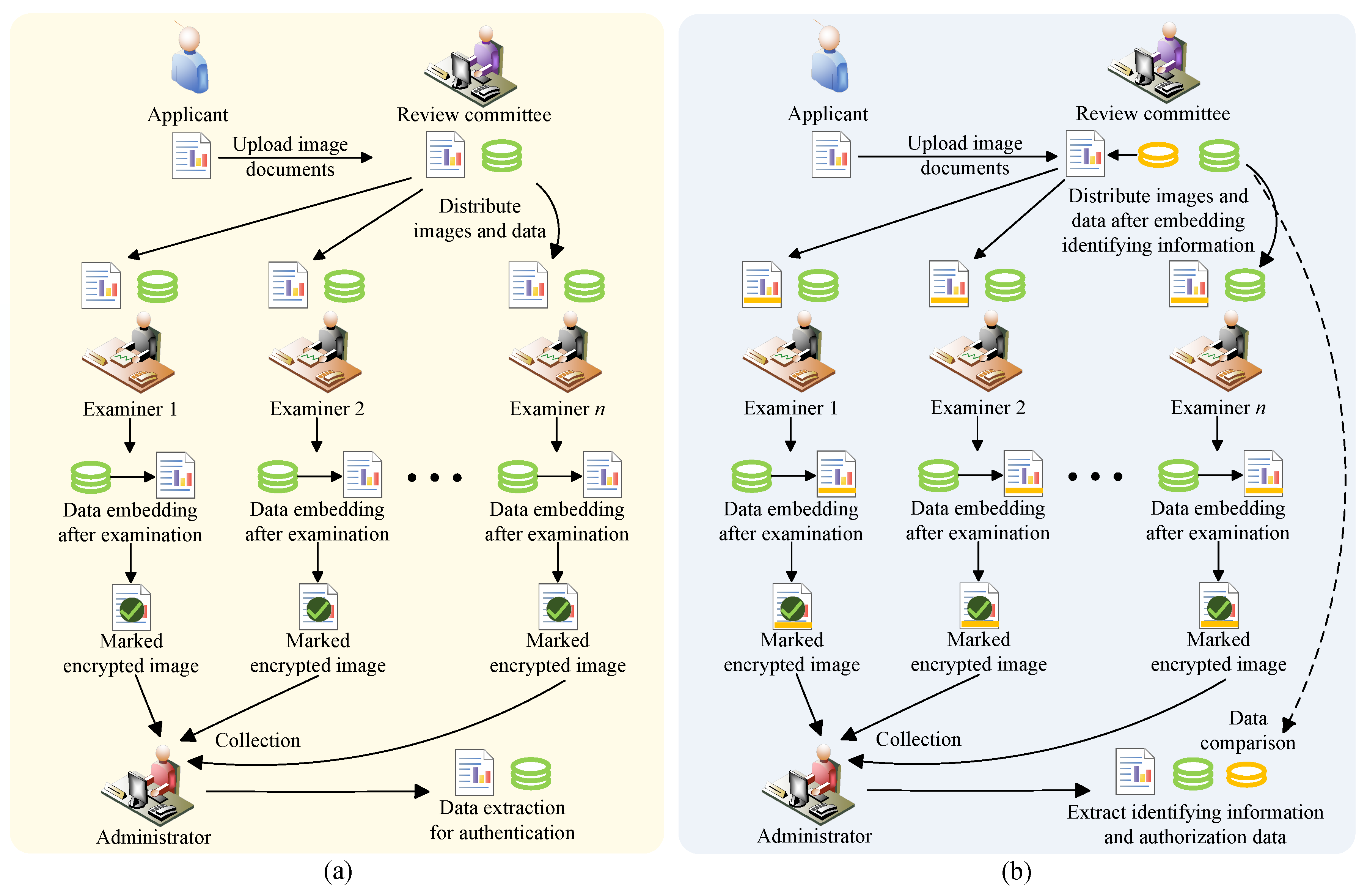
In 2020, Chen et al. introduced a hiding model based on secret sharing and multi-party embedding [19], distributing secret shares among various data hiders to achieve independent embedding. Zhao et al.’s algorithm adeptly conceals communication activities during multi-party data exchanges [20]. Xiong et al. [21] elaborated on the application of the RDH-EI algorithm in the context of the double-blind Inter Partes Review (IPR) scenario, as depicted in Figure 1a. The applicant entrusts the review committee with an encrypted image representing the patent file, which subsequently forwards the patent file and authorization data to each examiner. If the reviewer approves the patent, authorization data will be embedded into encrypted images to produce marked encrypted images. When the administrator extracts sufficient authorization data from the collected marked encrypted images, the patent passes the review. In 2022, Hua et al. [22] proposed an RDH-EI algorithm based on feedback secret sharing, enhancing the security of existing algorithms. Hua et al. [23] also proposed an RDH-EI scheme based on matrix-based secret sharing (MSS), enabling the complete restoration of the carrier image. In 2023, Yu et al. [24] proposed an RDH-EI scheme based on ciphertext sharing and hybrid coding to enhance embedding capacity. Hua et al. [25] also introduced a high-capacity RDH-EI scheme based on preprocessing-free secret sharing. However, secret sharing may reduce pixel correlation in the sub-secret image, resulting in wasted redundant space and potential security vulnerabilities. In cases of tampering during transmission, these algorithms may struggle to effectively detect such behavior due to the lack of a reference for confirmation, as both tampered and legitimate marked encrypted images appear visually indistinguishable as noisy images. This limitation compromises the ability to verify the authenticity of transmitted data in practical applications, posing security risks.

To address this issue, this paper proposes an RDH-EI algorithm based on adaptive median edge detection (AMED) and MSS secret sharing for distributed environments. Firstly, we introduce the innovative AMED pixel prediction technology, which achieves high prediction accuracy. Leveraging AMED technology and Huffman coding, we predict and recode the original image to generate the transitional image. Subsequently, using (r, n)-threshold MSS secret sharing in the $GF\left(2^8\right)$ domain, the transitional image is fragmented into n encrypted images, with identifying information embedded. The encrypted images are then distributed to individual data hiders, who independently embed secret data to acquire n marked encrypted images. Upon collecting r marked encrypted images, the original image can be reconstructed using the corresponding key, and the embedded data can be extracted. Discrepancies in the embedded identifying information before and after embedding can reveal tampering attacks. The algorithm is illustrated in the context of the IPR scenario in Figure 1b. Experimental results indicate a marked improvement in the embedding capacity of the proposed algorithm compared to the current algorithms [5,14,21,22,23,24]. Furthermore, the algorithm also possesses resilience, allowing up to $(n-r)$ fault points to occur.

Table 1. Comparison of previous algorithm limitations and solutions offered by our proposed algorithm.

RDH-EI Algorithms	Limitations	Approach to Problem-Solving
Puech et al. [4]	Low security	Using scrambling and exclusive or (XOR) encryption
Wang et al. [10] and Shirisha et al. [26]	Low prediction accuracy	Using AMED technology
Ren et al. [13]	High-entropy constraints on ciphertext state	Pre-encryption recoding
Zhang et al. [18]	Embedding rate constrained by image texture	Utilizing the characteristics of the cipher itself to embed data.
Yu et al. [24] and Hua et al. [25]	Inability to ensure data integrity	Designing identifying information for detection

outlines the limitations of previous algorithms and the solutions provided by the algorithm presented in this paper.

The main contributions of this paper’s algorithm are as follows:

• Introduction of the innovative AMED prediction technique, achieving superior prediction accuracy and surpassing the limitations of fixed predictors in existing MED techniques [15,26]. This enhancement significantly boosts the embedding capability of the algorithm.
• This article introduces an RDH-EI algorithm based on AMED prediction and MSS secret sharing, innovatively executing image segmentation within the $GF\left(2^8\right)$ domain. Compared to existing algorithms [23], the proposed method does not require additional data to store overflow pixels and avoids complex preprocessing, effectively reducing the usage of embedding space.
• The creative design of identifying information effectively enhances the monitoring of the security of the transmission environment and ensures the authenticity of the data.
• In comparison with existing algorithms, the algorithm proposed in this paper not only guarantees reversibility but also effectively increases embedding rates, thereby enhancing its practicality.

The subsequent sections of this paper unfold as follows: Section 2 elaborates on key technologies related to the algorithm, Section 3 specifies implementation details, Section 4 showcases experimental results and data analyses, and Section 5 concludes with a summary and outlook.

2. Key Technologies

2.1. MED Pixel Prediction

Pixel prediction techniques use known pixel values or contextual information to predict the value of a target pixel. When the predicted value closely matches the target pixel, it can be combined with coding strategies to achieve storage compression. This compression creates extra space that allows for the embedding of high-capacity secret data. Since its introduction by Li et al. [27], the MED predictor has been widely adopted in various data hiding algorithms due to its exceptional prediction accuracy [10,26]. In Figure 2, the MED predictor uses three neighboring pixel values around the target pixel $x(i,j)$ to estimate its value, resulting in the predicted value $px(i,j)$. The process of pixel prediction is detailed in the Equation (1).

$$px(i,j)=\left\{\begin{array}{c}max\left(x\right(i-1,j),x(i,j-1\left)\right) , if x(i-1,j-1)\le min\left(x\right(i-1,j),x(i,j-1\left)\right)\hfill \\ min\left(x\right(i-1,j),x(i,j-1\left)\right) , if x(i-1,j-1)\ge max\left(x\right(i-1,j),x(i,j-1\left)\right)\hfill \\ x(i-1,j)+x(i,j-1)-x(i-1,j-1), otherwise\hfill \end{array}\right.$$

(1)

In 2021, Wang et al. [10] introduced an RDH-EI algorithm that leverages this prediction technique, achieving an average embedding rate of 2.8764 bpp. Shirisha et al. [26] developed an RDH-EI scheme optimized for cloud service environments, combining the MED prediction technique with the logistic map’s sequence generation method to increase embedding capacity and ensure privacy protection during user information transmission, achieving a maximum embedding rate of 3.781 bpp. However, these algorithms typically identify embedding spaces based solely on local pixel correlation, without fully leveraging the distinct texture features of pixel blocks. To address this, the algorithm presented in this paper introduces the AMED prediction technique, incorporating adaptive parameters into the MED prediction method. This enhancement eliminates the limitations of fixed predictors, significantly improving pixel prediction accuracy and, consequently, the embedding rate of the RDH-EI scheme.

2.2. Matrix-Based Secret Sharing

In 2022, Hua et al. [23] introduced a secure $(r,n)$-threshold MSS scheme that leverages the invertibility of matrix operations and the uniqueness of their results. This scheme enhances secret sharing by incorporating a ciphertext feedback strategy, thereby significantly bolstering its security. Additionally, Hua et al. developed an RDH-EI scheme based on this secret sharing approach, which notably increased the embedding rate at that time. However, the scheme did not fully exploit the available redundant space during the encryption process. To optimize the utilization of this space, this paper employs the MSS technique to segment images in the domain $GF$(256) and embeds the identifying information during the segmentation process, consequently enhancing the algorithm’s security. The MSS scheme is constructed as follows:

Initially, an n × r matrix X is constructed so that the determinant of any n × r submatrix is coprime with F, following the outlined steps below:

• Generate n random positive integers $q_1$, $q_2$, …, $q_n$, each $q_k$ ($1\le k\le n$) being smaller than the prime F.
• Produce n distinct positive integers $p_1$, $p_2$, …, $p_n$, with each $p_k$ ($1\le k\le n$) also less than F.
• Initialize an n × r matrix where the first column is filled with the n integers $q_k$, and the elements of columns 2 through r are calculated using $x(i,j)$ = $x(i,j-1)$ × $(pi+j-2)$.

For partitioning the secret s, the sharing vector is constructed as $\mathit{a}={[s,a_1,\dots ,a_{r-1}]}^T$, where $a_1,\dots ,a_{r-1}$ are (r – 2) randomly chosen values. If the secret being shared is the first in a set, $a_1$ can be any value; otherwise, $a_1$ is a randomly chosen sub-secret from the previous secret, to incorporate ciphertext feedback for enhanced security. Secret sharing is executed according to the following equation, resulting in a vector $\mathit{f}={[f_1,f_2,\dots ,f_n]}^T$, which comprises n sub-secrets.

$$\mathit{f}=\mathit{X}\times \mathit{a}modF$$

(2)

The i-th sub-secret can also be computed from the following equation:

$$f_i=s\times x_{i1}+\sum _{j=2}^r{x}_{ij}{a}_{j-1} modF$$

(3)

Here, $x_{ij}$ represents the j-th element of the i-th row of the coefficient matrix X.

We assume that the receiver $P_i$ holds the sub-secret ($I{D}_i$, ${\mathit{f}}_i$), where i is the identification serial number. When r shares ($I{D}_1$, ${\mathit{f}}_1$), ($I{D}_2$, ${\mathit{f}}_2$), …, ($I{D}_r$, ${\mathit{f}}_r$) are collected, the first step involves generating the n × r coefficient matrix X. Then, the 1st, 2nd, …, r-th rows of matrix X are selected to construct the matrix Xr. The det(Xr) and F are mutually prime. The secret s can be obtained by the following equation:

$$\mathit{a}=\mathit{X}{\mathit{r}}^{-1}\times {\mathit{f}}^{\left(r\right)}modF$$

(4)

Here, ${\mathit{f}}^{\left(r\right)}={[f_1,f_2,\dots ,f_r]}^T$ represents a reconstructed vector of r sub-secrets. The first element of vector a is extracted to retrieve the secret s. In the context of an $(r,n)$-threshold MSS, any party with fewer than r sub-secrets cannot extract valid information, underscoring the algorithm’s robust tolerance and heightened security. The algorithm’s resilience and security are fortified by introducing random parameters during the encryption process for data embedding via data replacement. This embedding mechanism is incorporated into the proposed algorithm, augmenting its disaster resistance and enabling secure distributed data storage in cloud service environments.

3. The Proposed Method

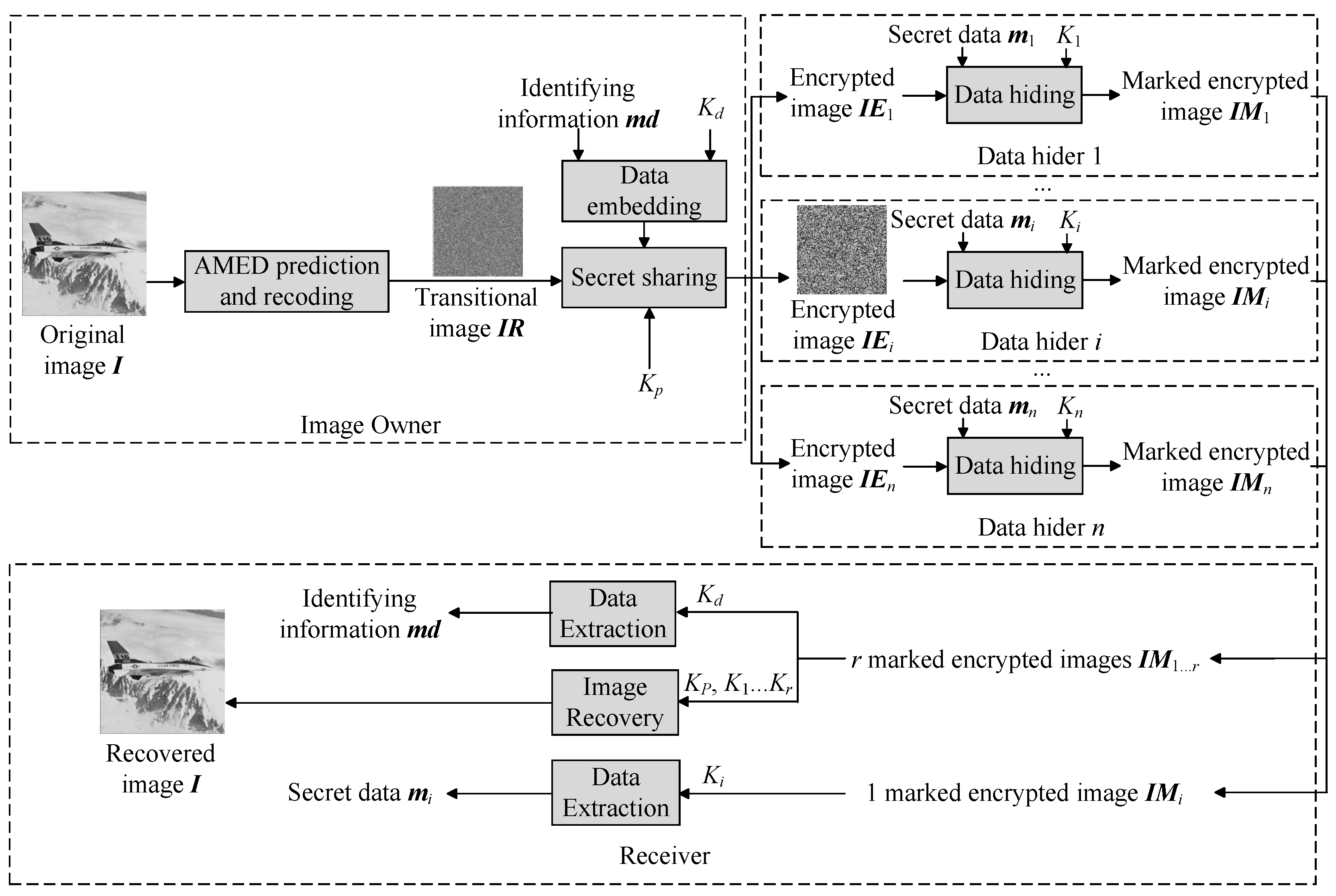
This study proposes an RDH-EI algorithm with a substantial embedding capacity, leveraging the correlation between image pixels and the encryption features of MSS. The algorithm’s framework is illustrated in Figure 3. Initially, the image owner preprocesses the original image I using the AMED pixel prediction technique, resulting in the transitional image IR. Subsequently, the image is shared using an $(r,n)$-threshold MSS, with the concurrent embedding of identifying information. Subsequent to this stage, the resulting n encrypted images ${\mathit{IE}}_k$ are distributed to individual data hiders for autonomous embedding, yielding n marked encrypted images ${\mathit{IM}}_k$. The recipient can leverage the key to extract the embedded secret data from each marked encrypted image individually or fully reconstruct the image to accurately extract both the secret data and identifying information by collecting any r marked encrypted images. Additionally, the recipient can detect tampering attempts in the transmission environment by comparing the identifying information pre- and post-embedding. The algorithm further utilizes the threshold characteristic of secret sharing to enhance data disaster resistance, accommodating up to $(n-r)$ failure points.

3.1. AMED Prediction and Recoding

3.1.1. Block-Level Pixel Prediction

To enhance the embedding capacity by leveraging pixel correlation, we employ direct pixel prediction on plaintext images. Initially, the carrier image I with dimensions $M\times N$ is partitioned into pixel blocks of size $B\times B$, where $B\ge 3$, resulting in $BM\times BN$ blocks. The block sizes BM and BN are determined by the following equation:

$$\left\{\begin{array}{c}BM=M÷B\hfill \\ BN=N÷B\hfill \end{array}\right.$$

(5)

To predict all pixels after block segmentation, we extend the pixel blocks as follows, so that edge pixels of the blocks also have reference pixels:

• When the pixel block contains the image pixel $x(1,1)$, the block is not expanded.
• When the pixel block does not contain the image pixel $x(1,1)$ but contains the pixel $x(1,j_0)$ with $j_0>1$, we add a column of random pixels to the left side of the pixel block, expanding it to a pixel block of size $B\times (B+1)$.
• When the pixel block does not contain the image pixel $x(1,1)$ but contains the pixel $x(i_0,1)$ with $i_0>1$, we add a row of random pixels on top of the pixel block, expanding it to a pixel block of size $(B+1)\times B$.
• Other cases: We add a column and a row of random pixels to the left and above the remaining pixel block, respectively, expanding it to a pixel block of size $(B+1)\times (B+1)$.

The target pixel $x(i,j)$ in the z-th pixel chunk is predicted using the AMED predictor to obtain the predicted value $px(i,j)$, as shown in Equation (6). Initially, the adaptive parameters $p_1$, $p_2$, and $p_3$ are determined, with their experimental values set to $p_1=0$, $p_2=0$, and $p_3=0$. These adaptive parameters remain constant when predicting pixels within the same pixel chunk.

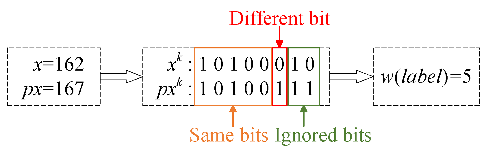
$$px(i,j)=\left\{\begin{array}{c}max(x(i-1,j),x(i,j-1))+p_1 , if x(i-1,j-1)\le min(x(i-1,j),x(i,j-1))\hfill \\ min(x(i-1,j),x(i,j-1))+p_2 , if x(i-1,j-1)\ge max(x(i-1,j),x(i,j-1))\hfill \\ x(i-1,j)+x(i,j-1)-x(i-1,j-1)+p_3, otherwise\hfill \end{array}\right.$$

(6)

The pixel value $x(i,j)$ is converted into an eight-bit binary string:

$$x^k(i,j)=⌊{\displaystyle \frac{mod(x(i,j),2^{9-k})}{2^{8-k}}}⌋,k=1,2,\cdots ,8$$

(7)

Here, $x_k(i,j)$ represents the value in the k-th bit plane, progressing from the highest bit, with $x_k(i,j)\in 0,1$. Similarly, transforming the predicted pixel value yields $p{x}_k(i,j)$, where k = 1, 2, …, 8. We compare $x_k(i,j)$ to $p{x}_k(i,j)$ bit by bit, starting from the most significant bit (MSB), to determine the number of consecutive identical bits and assign this as the label value $w(i,j)$ until a discrepancy is detected. The label value $w(i,j)$ ranges from 0 to 8, inclusive, where $w(i,j)=0$ indicates $x_k(i,j)\ne p{x}_k(i,j)$; $w(i,j)=8$ indicates $x(i,j)=px(i,j)$. For instance, considering the target pixel $x(i,j)=162$ and the predicted value $px(i,j)=167$. Comparing them reveals that the first five bits are identical, while the sixth bit differs, leading to a labeled value of w equal to 5. This process is illustrated in Figure 4:

AMED prediction is applied to all pixels within the pixel block, excluding those in the initial row and column, resulting in a total of ${(B-1)}^2$ tagged values and forming the tag map for the pixel block.

3.1.2. Calculating the Load Capacity for Secret Data of Pixel Blocks

We utilize Huffman coding to compress the labeled value w. There are nine potential values of w, thus necessitating nine distinct Huffman codes to represent these variations. Specifically, the codes 00, 01, 100, 101, 1100, 1101, 1110, 11110, 11111 are assigned to represent the nine encodings. The frequency of each label value within the pixel block is calculated, allowing for the use of shorter codes for labels with higher occurrence probabilities and longer codes for those with lower probabilities. Consequently, “0” is assigned to the label with the highest frequency, while “11111” corresponds to the least frequent label. For example, in a $64\times 64$ pixel block of a MAN image, following the successful prediction of pixel values, each pixel’s label is determined and encoded using Huffman coding. The statistical results illustrating the frequency distribution of label values within the block are provided in

Table 2. Pixel coding and load capacity statistics.

Label	Capacity (bits)	Distribution	Code	Code Length (bits)	Load (bits)
0	1	147	11111	5	−4
1	2	148	11110	5	−3
2	3	231	1110	4	−1
3	4	504	101	3	1
4	5	809	00	2	3
5	6	674	01	2	4
6	7	633	100	3	4
7	8	369	1101	4	4
8	8	454	1100	4	4

below.

Taking label $w=5$ as an illustration, based on the predicted pixel, we can deduce the highest six bits of the target pixel, enabling the substitution of these six bits with secret data for embedding. However, it remains imperative to record the label w utilizing the encoding “01”. Thus, for a solitary pixel possessing a label value of 5, its capacity to accommodate payload information can be expressed as $load(i,j)=5+1-2=4$. The load capacity of all pixels is computed according to Equation (8), yielding the data in column 6 of Table 2.

$$load(i,j)=\left\{\begin{array}{c}w+1-long\left(code\right(x(i,j)\left)\right),w\ne 8\hfill \\ w-long\left(code\right(x(i,j)\left)\right),w=8\hfill \end{array}\right.$$

(8)

Next, the load capacity of all pixels within the pixel block, excluding the first row and the first column, is computed to determine the pixel block’s load capacity, denoted as $load\left(z\right)$.

During the pixel prediction process, with the adaptive parameters fixed as $p_1=p_{10}$, $p_2=p_{20}$, and $p_3=p_{30}$, the load capacity of the pixel block, represented as $loa{d}_{p10,p20,p30}\left(z\right)$, is determined. The optimal parameter combination is identified through adaptive training. By traversing through all feasible values of $p_1$, $p_2$, and $p_3$, where the parameter values are constrained to integers from −3 to 4 (i.e., $p_i\in \mathbb{Z}$, $-3\le p_i\le 4$, resulting in a total of 24 potential combinations for the adaptive parameters $p_1$, $p_2$, and $p_3$ (i.e., $3\times 8=24$ possibilities). Consequently, there are 24 distinct values of $loa{d}_{p1,p2,p3}\left(z\right)$ for a pixel. Once these data reach their maximum value, the corresponding adaptive parameters are recorded as $p_1=p_{1n}$, $p_2=p_{2n}$, and $p_3=p_{3n}$. At this stage, the accuracy of the AMED median predictor is optimized, thereby maximizing the loading capacity of the image pixel block. The label value $w(i,j)$ is then designated as the final label for the pixels within the pixel block.

The method described above is applied to dynamically predict each pixel block of the original image, resulting in the derivation of labels for all pixels in the original image except those in the first row and column. This dataset is referred to as W. Subsequently, we document the optimal adaptive parameters that maximize the loading capacity.

3.1.3. Recoding

Initially, 3 bits are allocated to record the chunk size B. In the experiments outlined in this paper, B takes on values of 512, 256, 128, 64, and 32, which will be thoroughly elaborated on in the experimental section. Following this, $32\times BN\times BM$ bits are utilized to document the adaptive parameter ARP for all pixel blocks within the image, 32 bits are utilized to to record the Huffman coding rule (HCR). We convert W into a binary sequence WS, allocating an additional 22 bits to record the length of WS as $WL$. Finally, we concatenate $WL$, B, ARP, HCR, and WS in sequence with the pixel values of the first row and the first column of the original image to generate an edge information object identified as O.

Moving forward, we now proceed to integrate the edge information. Initially, we replace the pixel values of the first row and first column of the encrypted image with the first $8(M\times N-1)$ bits of the edge information O. Subsequently, leveraging the pixel label as a reference, we embed the remaining edge information into the encrypted image through bit substitution. This embedding takes place within the highest $(w+1)$ MSB of the unreplaced pixels in the encrypted image. The embedding formula is detailed as follows:

$${x_e}^{\prime }(i,j)=\left\{\begin{array}{c}{x}_e(i,j)mod{2}^{7-w}+{\displaystyle \sum _{l=0}^w}(s_l\times 2^{7-l}), 0\le w\le 6\hfill \\ {\displaystyle \sum _{l=1}^8}(s_l\times 2^{8-l}), 7\le w\le 8\hfill \end{array}\right.$$

(9)

The pixel value post-information embedding is represented as $x_e^{\prime }(i,j)$, where $s_l$ denotes the auxiliary information that can be embedded into the current pixel, and l signifies the load capacity of a single pixel. Following the embedding of all edge information, random noise is generated and embedded into the remaining positions post-edge information, as described in Equation (9), resulting in the transitional image denoted as IR.

3.2. Image Sharing and Identifying Information Embedding

In this study, the algorithm opts for $q=2_8$ to establish a finite field for executing secret sharing of the image within the domain. The image is divided into three parts: part A contains pixels with data WL, part B holds the remaining edge information, and part C encompasses the other pixels. For part B, a $(r,n)$-threshold secret sharing scheme is exclusively employed. Initially, a sequence of coefficient matrices $\mathit{Xs}={\mathit{X}}_1,{\mathit{X}}_2,\dots ,{\mathit{X}}_{LB}$ is generated based on the key $K_p$, where LB represents the number of pixels in part B. For segmenting pixel values $\mathit{IR}(i,j)$ and embedding identifying information, 8($r-1$) bits of data are extracted from the identifying information $\mathit{md}={0,1}^N$. After encryption with the identifying information hiding key $K_d$, every 8 bits are converted into decimal numbers, resulting in the sequence $\mathit{ms}=m{s}_1,m{s}_2,\dots ,m{s}_{r-1}$.

Then, the sharing vector ${\mathit{a}}_{ij}$ = [$\mathit{IR}(i,j)$, ${\mathit{a}}_1(i,j)$, …, ${\mathit{a}}_{r-1}{(i,j)]}^T$ is constructed, and the mapping $e_{ij}:(i,j)\to f_k(i,j)$ is generated by the key $K_p$, where $f_k(i,j)$ is the sub-secret of the previous pixel of pixel $\mathit{IR}(i,j)$, k is the position index of the sub-secret in the vector f, $k\in 1,2,\dots ,n$. When $\mathit{IR}(i,j)$ is the first pixel in part B, $f_k(i,j)$ is a random value. Calculate $a_1(i,j)$ with $a_2(i,j),a_3(i,j),\dots ,a_{r-1}(i,j)$, $h\in 1,2,\dots ,r-1$ from the following equation:

$$\left\{\begin{array}{c}{a}_1(i,j)=f_k(i,j)+m{s}_1\hfill \\ a_h(i,j)=m{s}_h\hfill \end{array}\right.$$

(10)

Determine ${\mathit{X}}_k$, $k\in 1,2,\dots ,LB$ in the generated sequence of Xs from the positional ordinal number of pixel $\mathit{IR}(i,j)$ in the pixel of part B. Finally, we perform secret sharing according to the equation, and embed ms:

$$\left(\begin{array}{c}{f}_1(i,j)\\ f_2(i,j)\\ ⋮\\ f_n(i,j)\end{array}\right)=\left(\begin{array}{cccc}{x}_{11}& x_{12}& \dots & x_{1r}\\ x_{21}& x_{22}& \dots & x_{2r}\\ ⋮& ⋮& \ddots & ⋮\\ x_{n1}& x_{n2}& \dots & x_{nr}\end{array}\right)\times \left(\begin{array}{c}\mathit{IR}(i,j)\\ a_1(i,j)\\ ⋮\\ a_{r-1}(i,j)\end{array}\right)modq$$

(11)

Once all pixel values in part B have been shared, $f_k(i,j)$ of the same identity k are aggregated to obtain n sub-secrets ${\mathrm{B}}_k$ of part B. These are then combined with parts A and C to generate n encrypted images ${\mathit{IE}}_k$, which are distributed by the image owner to n data hiders.

3.3. Secret Data Hiding

As a data hider $I{D}_i$, the secret data ${\mathit{m}}_i={0,1}^N$ is first encrypted using the data hiding key $K_i$ to produce the encrypted data ${\mathit{m}}_i^{\prime }={0,1}^N$. Subsequently, the partial edge information can be extracted from the first row and column of the encrypted image, containing parameters such as $WL$, B, ARP, HCR with the partial WS. By converting pixel values to 8-bit binary according to Equation (7), based on the partial WS, and referencing the HCR, the labeled values of the partial pixels can be determined, indicating the embedding positions of these pixels, specifically the high $(w+1)$ bits of the pixel values. By iteratively extracting and processing the edge information, all embedded edge information can be obtained.

Then we divide the image ${\mathit{IE}}_k$ into part A, part ${\mathrm{B}}_k$, and part C, and replace the pixel values of part C with ${\mathit{m}}_i^{\prime }$ to complete the embedding operation to obtain the embedded image ${\mathit{IA}}_k$, and then we perform the double encryption of scrambling encryption and XOR encryption to further improve the security of the embedded image. We first divide the image ${\mathit{IA}}_k$ into pixel blocks of size $B\times B$, use the key $K_i$ to generate a random number sequence, and then sort the random number sequence to obtain the index vector of the pixel blocks. Finally, the image blocks are scrambled according to the index vector to obtain the image ${\mathit{IE}}_k^{\prime }$. Then, we perform XOR encryption on the image: generate an $M\times N$ random matrix ${\mathit{P}}_k$ according to the key $K_i$, and encrypt the image ${\mathit{IE}}_k^{\prime }$ according to the following equation, finally obtaining marked encrypted images ${\mathit{IM}}_k$:

$${\mathit{IM}}_k(i,j)={\mathit{P}}_k(i,j)\oplus \mathit{IE}{ }_k^{\prime }(i,j)$$

(12)

The operation denoted by ⊕ corresponds to modulo 256 addition, with $i,j$ representing the position index where $1<i\le M$, $1<j\le N$.

3.4. Data Extraction and Image Recovery

Based on the possession of specific keys, the receiver can extract secret data from any marked encrypted image, or extract identifying data from r marked encrypted images and reconstruct the original image.

3.4.1. Secret Data Extraction

In the role of the recipient, the initial step involves employing the key $K_{si}$ to perform inverse scrambling and XOR decryption on the marked encrypted image ${\mathit{IM}}_k$, resulting in the recovery of the image ${\mathit{IA}}_k$. Subsequently, the receiver implements analogous procedures to those used during the secret data embedding phase to extract both the edge information $\mathit{O}$ and the encrypted data $\mathit{m}{’}_i$. Finally, decryption of $\mathit{m}{’}_i$ is carried out with the key $K_{si}$ to unveil the secret data ${\mathit{m}}_i$.

3.4.2. Image Recovery

The recipient independently conducts the aforementioned procedures on each of the r-marked encrypted images to isolate the portion ${\mathrm{B}}_{\mathrm{k}}$ from the images.

The identifiers for the data hiders are denoted as $i_1$, $i_2$, …, $i_r$, respectively. Utilizing the key $K_p$, we generate $\mathit{Xs}={\mathit{X}}_1,{\mathit{X}}_2,\dots ,{\mathit{X}}_{LB}$, and then select the $i_1,i_2,\dots ,i_r$ rows from the coefficient matrix ${\mathit{X}}_i$ to form the matrix ${\mathit{Xr}}_i$. The inverse matrix ${\mathit{Xr}}_i^{-1}$ is then calculated using the following equation:

$${\mathit{Xr}}_i^{-1}={\displaystyle \frac{{\mathit{Xr}}_i^{*}}{det({\mathit{Xr}}_i)}} mod256$$

(13)

where ${\mathit{Xr}}_i^{*}$ represents the accompanying matrix of ${\mathit{Xr}}_i$. Next, we utilize the ${\mathrm{B}}_{\mathrm{k}}$ part of the r embedded images ${\mathit{IA}}_k$ to decrypt and restore pixel $\mathit{IR}(i,j)$. Assuming pixels $f_1(i,j)$, $f_2(i,j)$, …, $f_r(i,j)$ are utilized for decryption, $\mathit{IR}(i,j)$ is obtained from the Equation (14):

$$\left(\begin{array}{c}\mathit{IR}(i,j)\\ a_1(i,j)\\ ⋮\\ a_{r-1}(i,j)\end{array}\right)={\mathit{Xr}}_i^{-1}\times \left(\begin{array}{c}{f}_1(i,j)\\ f_2(i,j)\\ ⋮\\ f_r(i,j)\end{array}\right) mod256$$

(14)

We conduct the recovery operation on all pixels to obtain the transitional image IR. Subsequently, we replace the corresponding pixel values in image IR with the first row and column pixels of the original image found in the edge information O. The adaptive parameters $p_1$, $p_2$, and $p_3$ corresponding to pixel $x’(i,j)$ can be obtained from the ARP in O. Starting from pixel $\mathit{IR}(2,2)$, the AMED prediction is performed on pixel $x’(i,j)$ in the order of top-to-bottom and left-to-right, and the predicted value $px(i,j)$ can be obtained. From the pixel label value w in the edge information, the load capacity $load\left(z\right)$ of the pixel can be obtained so that we can recover the pixel value of the original image because the predicted pixel is the same as the original pixel with the high w bits, and the $(w+1)$-th MSB is inverted. The recovery process unfolds in the following manner:

$$x(i,j)=\left\{\begin{array}{c}⌊{\displaystyle \frac{px(i,j)}{2^{8-w}}}⌋\times 2^{8-w}+b_{w+1}\times 2^{7-w}+x^{\prime }(i,j)mod{2}^{7-w},if0\le w\le 7\hfill \\ px(i,j),ifw=8\hfill \end{array}\right.$$

(15)

where $b_{w+1}$ is the $(w+1)$-th MSB flip value of the predicted pixel $px(i,j)$ as shown in the following equation:

$$b_{w+1}=\left\{\begin{array}{c}0 , p{x}^{w+1}(i,j)=1\hfill \\ 1 , p{x}^{w+1}(i,j)=0\hfill \end{array}\right.$$

(16)

Upon the successful recovery of all pixels, the original image I can be obtained.

3.4.3. Identifying Information Extraction

To illustrate the extraction process of the identifying information embedded in the transitional image pixel $\mathit{IR}(i,j)$, consider the extraction of $\mathit{IR}(i,j),a_1(i,j),\dots ,a_{r-1}(i,j)$ as per Equation (14). Subsequently, the key $K_p$ defines the mapping $e_{ij}$, enabling the derivation of $f_k(i,j)$ from $a_1(i,j)$. By following the procedure outlined in Equation (17), the encrypted identifying information $m_1$ can be obtained:

$$m{s}_1=a_1(i,j)-f_k(i,j)$$

(17)

Following this, the application of Equation (10) enables the computation of $m{s}_2$, …, $m{s}_{r-1}$. Subsequently, decrypting the data using the key $K_d$ reveals part of the identifying information md. This operation is repeated to extract all the identifying information, and it is compared with the md prior to embedding. Consistency denotes a secure transmission environment, whereas discrepancies point towards a potential data tampering attack during data transmission.

The receiver can independently perform secret data extraction, image recovery, and identifying information extraction based on possessing the key. These operations can be conducted separately.

4. Experiments and Analysis of Results

For the assessment of the algorithm’s efficacy and to highlight its advancements over current methodologies, a total of 21,338 8-bit grayscale images were selected from three image datasets: BOSSBase [28], BOWS-2 [29], and UCID [30], for testing and comparison in experiments. The primary set of six test images utilized in these experiments are presented in Figure 5. The evaluation of the algorithm’s performance in this research focuses on four crucial aspects: reversibility, data embedding efficiency, data expansion, and security.

The experimental setup utilized an Intel® Core™ i5-9300H CPU (Lenovo, Beijing, China) operating at 2.40 GHz, equipped with 8 GB of memory, running on the Windows 11 platform, and utilizing the MATLAB R2021b simulation environment.

4.1. Reversibility

In this study, we implemented the proposed algorithm, based on the (3, 4)-threshold, to conduct embedding simulation experiments using the Jetplane image. Figure 6 illustrates images generated at different stages of the experiments. The sequence begins with the original image shown in Figure 6a, followed by the transitional image post-pixel prediction and encoding in Figure 6b. Figure 6c–f display the marked encrypted images produced after embedding random data, from which human eyes cannot discern any identifiable information about the secret data or the original image. Figure 6g visualizes the recovered image.

To ascertain whether the recovered image exhibits significant distortion, we utilize the peak signal-to-noise ratio (PSNR) as a comparative metric between the recovered image and the original image, measuring the reversibility of the algorithm. Typically, when the PSNR approaches infinity, the original image is considered fully recovered. The PSNR is calculated using the following equation:

$$\mathrm{PSNR}=10\times {log}_{10}\left[{\displaystyle \frac{{(2^k-1)}^2}{MSE}}\right]$$

(18)

where 4 is the image pixel depth and MSE is the mean square error, which can be derived from the following equation:

$$MSE={\displaystyle \frac{1}{M\times N}}\sum _{i=0}^{M-1}{\sum _{j=0}^{N-1}\left[T_{i,j}-T{ }_{i,j}^{\prime }\right]}^2$$

(19)

where M and N denote the image size, $T_{ij}$ and $T_{ij}^{\prime }$ are the pixels of the original image and the pixels of the recovered image, respectively.

Figure 7 shows a comparison of the rate distortion curves of the algorithms on the Lena image. The algorithm developed by Sahu et al. [5] sustains a stable PSNR of approximately 40 dB during image recovery. The algorithm by Datta et al. [7] employs matrix encoding for embedding, resulting in distortion during image recovery, with an average PSNR of 72.52 dB. Additionally, the algorithm by Kamil et al. [14] achieves a PSNR of 58.7 dB at an embedding rate of 1 bpp. The algorithm by Zhang et al. [18] discards certain data regarding the original image during encoding and embedding, which leads to image distortion. Similarly, the approach by Xiong et al. [21] experiences difficulty in fully recovering the original pixel due to bit flipping, causing image distortion. In contrast, the algorithm presented in this paper is tested in Matlab simulation experiments, and the PSNRs obtained are all ∞ with full reversibility. In the theoretical derivation, Equations (11) and (14) are inverse operations to each other, which ensures that the extracted pixel $\mathit{IR}(i,j)$ has the same value as before encryption, and the process of encoding the original image I into the transitional image IR is reversible, so that the recovered image is the same as the original image. The algorithm in this study achieves lossless image recovery and outperforms existing methodologies.

4.2. Data Embedding Performance

The embedding rate (ER) serves as a critical metric for gauging the effectiveness of an information hiding algorithm, quantifying the average amount of information embeddable per pixel in an image. The embedding rate can be calculated as follows:

$$\mathrm{ER}={\displaystyle \frac{\mathrm{Total}\mathrm{number}\mathrm{of}\mathrm{embedded}\mathrm{bits}}{\mathrm{Total}\mathrm{number}\mathrm{of}\mathrm{pixels}\mathrm{of}\mathrm{the}\mathrm{encrypted}\mathrm{image}}}$$

(20)

We can theoretically calculate the ER of the algorithm proposed in this paper:

$$\mathrm{ER}={\displaystyle \frac{8(r-1)(MN-3)+8(1-r+n)⌊Load/\phantom{Load8}8⌋}{nMN}}$$

(21)

where $Load$ represents the total load capacity of the intermediate image, higher pixel prediction accuracy corresponds to a greater $Load$ value. It is evident that with other parameters unchanged, as the image size $MN$ increases, ER also increases. In practice, as the image size grows, the $Load$ value also increases, thereby increasing ER further. Additionally, the threshold values $(r,n)$ will cause nonlinear effects on ER depending on the actual sizes of other parameters.

Upon receiving the encrypted image, the information hider embeds the secret data by replacing bits in the image’s noisy regions. The quantity of embedded information correlates with the load capacity value of the intermediate image.

Table 3. Embedding rates and correlation statistics of different images.

Images	Total Capacity (bits)	Code Length (bits)	Extra Bits (bits)	Total Load (bits)	ERs (bpp)
Jetplane	1,590,321	792,651	633	797,037	5.5202
Man	5,622,829	3,118,402	2361	2,502,066	5.1931
Airplane	1,663,820	683,251	633	979,936	5.8690
Tiffany	1,537,779	785,567	633	751,579	5.4335
Baboon	1,085,666	796,502	633	288,531	4.5503
Lena	1,477,960	792,862	633	684,465	5.3055

presents the load capacities for various images when $B=64$. The load capacity for an image is not merely the sum of the pixel blocks’ load capacities, as additional space is required to store edge information, ensuring the algorithm’s ability to fully recover the original image. As seen in Table 3, the load capacity varies across images due to their distinct texture features. By employing the (3, 4)-threshold algorithm proposed in this paper for image embedding, it is clear that the algorithm demonstrates varying ERs across different images.

To assess the universality of the embedding capabilities of the algorithms proposed in this paper, we selected 10,000 grayscale images of size 512 × 512 from each of the BOSSBase and BOWS-2 databases, along with 1338 grayscale images of sizes $512\times 384$ or $384\times 512$ from the UCID database. These images were used to embed randomly generated information. According to the experimental findings presented in

Table 4. The embedding rates and peak signal-to-noise ratio of the algorithm proposed in this paper across various datasets.

Datasets	Threshold Value	Criteria	Best Case	Worst Case	Average
BOSSbase	(3, 4)	ER (bpp)	6.9487	4.3446	5.6934
		PSNR	∞	∞	∞
	(6, 6)	ER (bpp)	7.6495	6.7815	7.2311
		PSNR	∞	∞	∞
BOW-2	(3, 4)	ER (bpp)	6.8109	4.3259	5.6361
		PSNR	∞	∞	∞
	(6, 6)	ER (bpp)	7.6035	6.7752	7.2120
		PSNR	∞	∞	∞
USID	(3, 4)	ER (bpp)	7.3399	4.2752	5.8142
		PSNR	∞	∞	∞
	(6, 6)	ER (bpp)	7.7799	6.7583	7.2713
		PSNR	∞	∞	∞

, the minimum embedding rate of the algorithm for the (3, 4) threshold-exceeds 4 bpp, and the average embedding rate is over 5.5 bpp across all databases. For the (6, 6)-threshold, the minimum embedding rate exceeds 6.5 bpp, with an average rate over 7 bpp. Furthermore, the PSNRs for the algorithm are infinite, ensuring reversibility. The performance of the algorithms, in terms of embedding rates across the three image databases, is illustrated in Figure 8.

Next, we delve into the impact of the threshold values in secret sharing on the image embedding rate.

Table 5. Embedding rate under different parameters of the algorithm.

Threshold Value	$\mathit{B}=32$	$\mathit{B}=64$	$\mathit{B}=128$	$\mathit{B}=256$	$\mathit{B}=512$
(2, 2)	5.1978	5.1930	5.1897	5.1867	5.1839
(3, 3)	6.1318	6.1287	6.1265	6.1245	6.1226
(3, 4)	5.1978	5.1930	5.1897	5.1867	5.1839
(4, 4)	6.5989	6.5965	6.5948	6.5933	6.5919
(4, 5)	5.7582	5.7544	5.7518	5.7494	5.7471
(5, 5)	6.8791	6.8772	6.8759	6.8746	6.8735
(5, 6)	6.1318	6.1287	6.1265	6.124	6.1226
(5, 7)	5.5981	5.5940	5.5912	5.5886	5.5862
(6, 6)	7.0659	7.0643	7.0632	7.0622	7.0612
(6, 7)	6.3987	6.3960	6.3941	6.3924	6.3907
(6, 8)	5.8983	5.8947	5.8923	5.8900	5.8879
(12, 12)	7.5330	7.5327	7.5320	7.5311	7.5306
(12, 14)	6.7991	6.7975	6.7968	6.7949	6.7931
(12, 16)	6.2487	6.2370	6.2463	6.2426	6.2399

illustrates the comparative embedding rates of our algorithm in embedding experiments on Man image under different parameters. The experimental findings reveal that with a constant threshold value, smaller block sizes result in higher embedding rates. This phenomenon arises because the AMED prediction relies on texture features from different blocks; thus, the smaller the block size, the higher the prediction accuracy. Moreover, when the block size remains constant, holding an equal r value, lower n values correspond to higher embedding rates, and when n values remain the same, higher r values lead to higher embedding rates. The maximum embedding rate achieved by our algorithm in this experiment reaches up to 7.5330 bpp. In practical applications, it is essential to align the r and n values of the algorithm as closely as possible to ensure both resilience and a high embedding rate.

In order to demonstrate the superior embedding rate capabilities of our algorithm, we conducted experiments using six widely recognized images: Airplane, Baboon, Lena, Jetplane, Man, and Tiffany. The results, depicted in Figure 9, compare the highest embedding rate achieved by our algorithm with those of existing algorithms. Sahu et al. [5]’s algorithm utilized LSB matching for embedding, achieving a modest embedding rate of 2 bpp. Kamil et al. [14]’s algorithm attained an average embedding rate of 0.90 bpp, primarily due to less advanced compression technologies. Xiong et al. [21]’s algorithm encoded pixels into multiple Hamming code words and leveraged error correction capabilities, reaching embedding rates of up to 3 bpp. In the experiments, our algorithm excelled with a maximum embedding rate of 7.11 bpp, doubling the rate of Xiong et al. [21]’s approach. While algorithms in references [22,23] both utilized image correlation embedding post secret sharing, their embedding rates are constrained by coding techniques. Yu et al. [24] improved upon this by employing a hybrid coding technique, achieving an average embedding rate of up to 3.20 bpp with a (3, 4) threshold. Our algorithm, using the same threshold values, surpasses Yu et al.’s by approximately 2.12 bpp. Notably, our algorithm based on (6, 6)-threshold achieves an average embedding rate exceeding 7 bpp across these six images, significantly outperforming existing algorithms. This marked advancement positions our algorithm as a more practical solution, capable of embedding significantly larger volumes of data within images.

4.3. Data Expansion

We use the data expansion rate to measure the resources occupied by marked encrypted images, which is expressed as the ratio of ciphertext data volume to original image data volume. Based on the embedding operation phase, our algorithm belongs to the category of VRIE and VRAE. We compare our algorithm with existing ones. Experimental results are shown in

Table 6. Comparison of data expansion rates for different algorithms.

Algorithms	Type	Encryption Methods	Relative Expansion Rate	Total Expansion Rate
Kamil et al. [14]	VRBE	Stream cipher	1	1
Ke et al. [12]	VRIE	Homomorphic encryption	256	256
Xiong et al. [21]	VRAE	Secret sharing	1	n
Hua et al. [22]	VRAE	Secret sharing	$1/(r-1)$	$n/(r-1)$
Hua et al. [23]	VRAE	Secret sharing	1	n
Yu et al. [24]	VRAE	Secret sharing	1	n
Proposed	VRIE + VRAE	Secret sharing	1	n

. An exemplary algorithm by Kamil et al. [14] achieves embedding via histogram shifting, categorized as a VRBE algorithm, with the resulting marked encrypted images retaining the size of the original images. Conversely, Ke et al.’s algorithm [12] leverages homomorphic encryption schemes, achieving a notable data expansion rate of up to 256, with limited practical utility. The algorithm proposed in references [21,23,24] and the algorithm presented in this paper both perform embedding operations on sub-secret images, with the total ciphertext data volume being the number of shares n. However, for each distributed storage, the data expansion rate is 1. Our algorithm embeds identifying information during secret sharing and embeds the user’s secret data after encryption through bit replacement, with neither embedding process altering the image size; the only data expansion occurs during secret sharing. While our algorithm and existing RDH-EI algorithms share comparable data expansion rates, ours excels in image recovery quality and embedding rates, thereby delivering superior performance.

4.4. Security

4.4.1. Computational Complexity

Computational complexity denotes the computational workload needed to execute an algorithm and serves as a pivotal metric for assessing performance. Presently, stream ciphers and public key cryptography algorithms are prevalent in the RDH-EI algorithm domain.

Table 7. Computational complexities of different RHD-EI algorithms.

Algorithms	Encryption Methods	Computational Complexity
		Data Embedding	Data Extraction	Image Recovery
Puech et al. [4]	AES encryption	$O\left(1\right)$	$O\left(1\right)$	$O\left(1\right)$
Ke et al. [8]	LWE encryption	$O\left(N^2\right)$	$O\left(1\right)$	$O\left(N^2\right)$
Ren et al. [13]	Paillier encryption	$O\left(N^3\right)$	$O\left(1\right)$	$O\left(N^3\right)$
Chen et al. [19]	Shamir Secret sharing	$O\left(N\right)$	$O\left(1\right)$	$O\left(N{\log }^2\mathit{N}\right)$
Hua et al. [22]	CFSS Secret sharing	$O\left(N\right)$	$O\left(1\right)$	$O\left(N{\log }^2\mathit{N}\right)$
Proposed	MSS Secret sharing	$O\left(N\right)$	$O\left(N^2{\log }^2\mathit{N}\right)$	$O\left(N{\log }^2\mathit{N}\right)$

displays the computational complexity of executing the algorithm across various encryption methodologies.

AES encryption and decryption of a pixel exhibit a computational complexity of $O\left(1\right)$. When considering a private key length of r, the computational complexities for encrypting and decrypting a pixel using LWE and Paillier encryption methods are $O\left(r^2\right)$ and $O\left(r^3\right)$, respectively. Employing $(k,n)$-threshold secret sharing encryption for a pixel results in a computational complexity of $O\left(n\right)$ for encryption and $O\left(n{\log }^2\mathit{n}\right)$ for decryption, as rigorously proven by Shamir et al. [31].

In our algorithm, the computational complexity of AMED prediction and re-encoding operations is $O\left(1\right)$. During the secret splitting process, data embedding occurs by establishing a mapping relationship between secret data and vector parameters, maintaining a computational complexity of $O\left(n\right)$. Information extraction involves recovering non-leading parameters of the shared vector; Hua et al. [23] proposed a recursive algorithm with a computational complexity of $O\left(k^2{\log }^2\mathit{k}\right)$. For image recovery, only the leading parameter of the shared vector is necessary, mirroring the process in MSS secret sharing, showcasing a computational complexity of $O\left(k{\log }^2\mathit{k}\right)$.

4.4.2. Extraction Correctness

The legitimate receiver can successfully extract the encrypted secret data ${\mathit{m}}_i^{\prime }$ from the marked encrypted image using the authorized key $K_{si}$, while an attacker remains unable to extract the secret data accurately.

Assuming an attacker attempts to decrypt ${\mathit{m}}_i^{\prime }$ using a forged key, the extracted secret is compared bit by bit with ${\mathit{m}}_i$. If they match, it is marked as 0; otherwise, it is marked as 1. Experimental results in Figure 10a show that occurrences of 1 and 0 have equal probabilities of 0.5 and are entirely independent. When the receiver uses the data hiding key $K_{si}$ for decryption and extraction, the extracted data match the pre-embedding data, demonstrated in Figure 10b. This underscores that without $K_{si}$, attackers cannot extract valid information from the marked encrypted image, thus fortifying the algorithm against unauthorized access. Only with a valid key can the receiver accurately retrieve the secret data. If an attacker tampers with a marked encrypted image, the algorithm detects such alterations by comparing identifying information before and after embedding. When the algorithm’s threshold is set to (3, 4), we forge a random image and perform identifying information extraction alongside any two legitimate marked encrypted images. Subsequently, we compare the extracted data with the pre-embedding identifying information from each image. The result, as shown in Figure 10c, reveals significant differences, indicating the receiver’s inability to extract correct identifying information. Choosing any three marked encrypted images for decryption, the experiment demonstrates that the extracted identifying information aligns with the pre-embedding identifying information, as depicted in Figure 10d. When an attack takes place during the transmission of encrypted images from the image owner to the data hider, we manipulate any encrypted image to replicate this process, and involve this image in the subsequent process of embedding and extracting secret data. By analyzing identifying information, we can determine the occurrence of the attack, as illustrated in Figure 10e. Conversely, when no attack is present, the experimental results are depicted in Figure 10f. This suggests that the algorithm can effectively detect potential malicious activities in the transmission environment using identifying information, thus verifying the authenticity of the data.

Due to the threshold nature of the described algorithm, the successful extraction of secret data requires multiple users to simultaneously provide the decryption keys needed. However, managing multiple users can introduce significant complexity, potentially leading to conflicts such as resource contention from concurrent decryption attempts. To address this challenge, we conducted experiments with existing distributed locks, and through comparison, found that Redisson distributed lock can effectively handle concurrent access among multiple users while minimizing related complexities [32].

Table 8. Comparison results between Redisson distributed lock and other distributed locks.

Other Existing Distributed Locks	Disadvantages	Redisson Distributed Lock Advantages
ZooKeeper distributed lock [33]	Relies on external storage media, increasing system development costs	Built-in complete persistence support
Memcached distributed lock [34]	Slower response speed	Fast response speed and low latency
Hazelcast distributed lock [35]	Lacks flexibility	Suitable for a wider range of scenario needs
Apache Curator distributed lock [36]	Complex deployment	Simple and easy to use
Etcd distributed lock [37]	Lacks fault tolerance	High fault tolerance, supports fine-grained lock control

presents the experimental results, showcasing that Redisson distributed lock offers benefits such as fast response times, simplicity of operation, and support for fine-grained lock control, making it better-suited for serving multiple users in the RDH-EI algorithm. The implementation of Redisson distributed lock involves locking the system during secret data extraction operations. We employed the (3, 4)-threshold algorithm in this paper to embed random data into large images, followed by simultaneously having two groups of users apply for system occupation and locking. We designated the thread that first occupies the system as Thread A and the unsuccessful one as Thread B. We set time points to observe the behavior of Thread B, and the results are shown in

Table 9. Results of concurrent user access under Redisson distributed lock.

Timestamps	Behavior of Thread B after Attempting to Lock	Remaining Time for the Lock to Expire
t = 5.00 s	Failed locking attempt, message subscription for listening	25.04 s
t = 10.00 s	Listening	29.97 s
t = 15.00 s	Listening	24.98 s
t = 25.00 s	Listening	25.04 s
t = 30.00 s	Listening	19.94 s
t = 50.00 s	Successful locking, system occupation	30.00s
t = 55.00 s	Occupying the system	25.83 s
t = 65.00 s	Occupying the system	26.00 s

.

When Thread A successfully occupies the system and locks it, the system sets the leaseTime to 30 s and activates a watchDog that renews the lock every 10 s to maintain a timeout of 30 s. Meanwhile, Thread B fails to lock and subscribes to listen for release notifications of the lock. When the system lock is released, a broadcast message is sent out. As Thread A occupies the system for 10 and 20 s, the watchDog extends the lock duration to 30 s, while Thread B continues to listen. Around the 50 s mark, when Thread A completes its operation and releases the lock, Thread B receives the broadcast, attempts to acquire the lock, succeeds, and starts its operation, with the watchDog also kicking in. Experimental results demonstrate that Redisson distributed lock effectively resolves coordination issues among multiple users.

4.4.3. Uncertainty

To prevent attackers from retrieving accurate information from the marked encrypted image, it is imperative that the digital attributes of the image align closely with those of a randomly generated noise image. This has been empirically examined from three distinct perspectives: pixel distribution, correlation, and information entropy. We embed randomly generated identifying information and secret data into the Man image using our algorithm based on a (3, 3) threshold. Figure 11 demonstrates the pixel distribution in the correlation image, indicating that the pixel values are uniformly distributed in both the encrypted image and the marked encrypted images.

Next, we leverage the security of the pixel correlation analysis algorithm. We randomly select 26,000 pairs of adjacent pixels in the original image and the marked encrypted image with embedded secret data, analyzing the correlation coefficients in three directions: horizontal, vertical, and diagonal. The formula below represents the correlation coefficient $r_{xy}$.

$$\begin{array}{c}{r}_{xy}={\displaystyle \frac{\mathrm{cov}(x,y)}{\sqrt{D\left(x\right)}\sqrt{D\left(y\right)}}}\hfill \\ D\left(x\right)={\displaystyle \frac{1}{N-1}}{\displaystyle \sum _{i=1}^N}{(x_i-E\left(x\right))}^2\hfill \\ D\left(y\right)={\displaystyle \frac{1}{N-1}}{\displaystyle \sum _{i=1}^N}{(y_i-E\left(y\right))}^2\hfill \\ \mathrm{cov}(x,y)={\displaystyle \frac{1}{N-1}}{\displaystyle \sum _{i=1}^N}(x_i-E\left(x\right))(y_i-E\left(y\right))\hfill \\ E\left(x\right)={\displaystyle \frac{1}{N}}{\displaystyle \sum _{i=1}^N}{x}_i,E\left(y\right)={\displaystyle \frac{1}{N}}{\displaystyle \sum _{i=1}^N}{y}_i\hfill \end{array}$$

(22)

where x and y represent the values of the paired neighboring pixels in the test image.

Table 10. Correlation coefficient of test images.

Direction	Original Image	Encrypted Image	Marked Encrypted Image I	Marked Encrypted Image II	Marked Encrypted Image III	Average of the Marked Encrypted Images
horizontal	0.9582	0.0015	0.0019	0.0027	0.0022	0.0023
vertical	0.9656	0.0016	0.0033	0.0025	0.0026	0.0028
diagonal	0.9382	0.0021	0.0015	0.0019	0.0027	0.0021

presents the correlation coefficient test results for the Man image. These results reveal that the correlation coefficients of the original image demonstrate strong correlations in various directions, with an average value of 0.9540, nearing 1. In contrast, the correlation coefficients of the marked encrypted images approach 0 in different directions, indicating a significant reduction in correlation. Figure 12 displays the scatter plot of the correlation coefficients for both the original and the marked encrypted images. It is observed that most samples from the original image cluster around the line $y=x$, indicating a strong correlation. Meanwhile, the scatter plots for the marked encrypted images show a uniform distribution, aligning with the mathematical statistical characteristics of random grayscale images. This outcome results from the algorithm’s process of embedding secret data into the image, disrupting its pixel correlation, and subsequently performing XOR encryption on the encrypted images, further diminishing the pixel correlation coefficient to nearly zero.

In practical application scenarios, algorithms often face unknown attacks. Therefore, we use Spearman’s rank correlation coefficient (SRCC) and Kendall rank correlation coefficient (KRCC) [38] to test the monotonicity of images, further assessing whether attackers can extract information about the original images. Experimental results are shown in

Table 11. SRCC and KRCC evaluation of the (3, 3)-threshold algorithm in this study.

Images	SRCC (%)			KRCC (%)
	${\mathit{IM}}_{\mathbf{1}}$	${\mathit{IM}}_{\mathbf{2}}$	${\mathit{IM}}_{\mathbf{3}}$	${\mathit{IM}}_{\mathbf{1}}$	${\mathit{IM}}_{\mathbf{2}}$	${\mathit{IM}}_{\mathbf{3}}$
Baboon	−0.4528	0.0715	0.1518	0.5626	−0.2253	0.0455
Tiffany	0.5549	0.2561	0.0842	0.2151	0.4158	0.0454
Man	0.3254	0.2545	0.0325	0.1256	0.1654	0.0532
Airplane	0.2395	0.0389	0.1523	0.0654	0.3622	0.5696
Jetplane	0.6915	0.2892	0.6512	0.0715	0.0312	0.5782
Lena	0.2746	0.3625	0.0214	0.1547	0.5154	0.0354

, where [38] indicates the following: when SRCC and KRCC are close to 1 or −1, there is a high correlation between images, while values close to 0 indicate low correlation. In our algorithm, both the SRCC and KRCC values of the marked encrypted images ${\mathit{IM}}_i$ are close to 0. This can be attributed to the encrypted secret data displaying pseudo-random characteristics before embedding, while the algorithm maintains the ciphertext feedback properties of the MSS secret sharing scheme, along with certain scalability attributes. As a result, our algorithm demonstrates robust security.

The information entropy of an image represents the balance in the occurrence frequency of each grayscale level of its pixels. A higher information entropy value indicates a greater amount of information contained in the image and better defense against statistically based attacks. The information entropy is calculated using the following equation:

$$H=-\sum _{i=1}^{N}Pr\left({\sigma }_i\right)logPr\left({\sigma }_i\right)$$

(23)

where N represents the number of pixel values, ${\sigma }_i$ denotes the i-th pixel value, and Pr$\left({\sigma }_i\right)$ signifies the probability of the i-th pixel value occurring.

For a grayscale image with an 8-bit depth, where the pixel values ${\sigma }_i$ range from 1 to 255, the information entropy reaches its peak when the probability Pr$\left({\sigma }_i\right)$ equals 1/256, resulting in a maximum entropy value of 8. In our experiment, we assessed the information entropy of the pertinent images, with the results detailed in

Table 12. Information entropy of test images.

Carrier Image	Original Image	Encrypted Image	Marked Encrypted Image I	Marked Encrypted Image II	Marked Encrypted Image III	Average of the Marked Encrypted Images
Lena	7.4456	7.9911	7.9912	7.9913	7.9915	7.9913
Baboon	7.3577	7.9917	7.9912	7.9916	7.9911	7.9913
Man	7.3013	7.9916	7.9913	7.9915	7.9917	7.9915
Goldhill	7.4778	7.9917	7.9915	7.9915	7.9912	7.9914

. The average information entropy of the marked encrypted images was determined to be 7.9914, closely approaching the theoretical maximum of 8, indicating a uniform distribution of pixel values. This algorithm effectively shields the image and secret data from statistic-based attacks, demonstrating robust security.

4.4.4. Differential Attack

To evaluate the resistance of the proposed algorithm against differential attacks, we employ the metrics of the number of pixel change rate (NPCR) and the uniform average change intensity (UACI) [39]. NPCR quantifies the rate of pixel modifications observed at corresponding locations between the original and encrypted images; a value closer to 100% signifies greater discrepancies between the images, reflecting a higher level of security for the algorithm. On the other hand, UACI calculates the average difference in pixel values across the two images. As per the findings by Wu et al. [39], the optimal NPCR and UACI values for a secure encryption algorithm are 99.609% and 33.464%, respectively.

In our study, we have implemented the (4, 5)-threshold algorithm detailed in the paper to embed random data into the six images depicted in Figure 5, with a fixed condition of B = 32. Following this, we conducted experimental assessments to ascertain the NPCR and UACI of the algorithm, the results of which are summarized in

Table 13. The embedding rates and peak signal-to-noise ratio of the algorithm proposed in this paper across various datasets.

Images	NPCR (%)					UACI (%)
	${\mathit{IM}}_{\mathbf{1}}$	${\mathit{IM}}_{\mathbf{2}}$	${\mathit{IM}}_{\mathbf{3}}$	${\mathit{IM}}_{\mathbf{4}}$	${\mathit{IM}}_{\mathbf{5}}$	${\mathit{IM}}_{\mathbf{1}}$	${\mathit{IM}}_{\mathbf{2}}$	${\mathit{IM}}_{\mathbf{3}}$	${\mathit{IM}}_{\mathbf{4}}$	${\mathit{IM}}_{\mathbf{5}}$
Airplane	99.6853	99.6512	99.6452	99.6021	99.5324	33.4852	33.1220	33.6542	33.4526	33.7512
Baboon	99.5624	99.6452	99.6975	99.5135	99.4965	33.8102	33.5615	33.6412	33.2351	33.1522
Lena	99.5621	99.4860	99.6541	99.7031	99.6514	33.5615	33.8143	33.2545	33.3254	33.8472
Jetplane	99.7112	99.6421	99.5815	99.3215	99.6256	33.6781	33.2548	33.8972	33.2482	33.7957
Tiffany	99.5568	99.5406	99.6452	99.5945	99.6512	33.2418	33.5751	33.7251	33.1241	33.7512
Man	99.5612	99.6425	99.7029	99.5612	99.4942	33.1458	33.5216	33.5782	33.9875	33.5442

. Our algorithm showcases NPCR and UACI values closely tracking 99.609% and 33.464%, respectively, thus affirming its effectiveness in thwarting differential attacks. Noteworthy is the fact that the algorithm’s ciphertext feedback mechanism induces notable modifications in the encrypted image even in the presence of minor fluctuations in the plaintext image. Moreover, the algorithm discussed in this paper integrates encoding techniques, scrambling encryption, and XOR encryption, culminating in a robust and indeterminate system with enhanced security measures.

We have demonstrated through simulation the effectiveness of our algorithm in a controlled environment, but real-world validation in diverse and dynamic environments might reveal additional practical challenges and limitations. However, the validation of the algorithm is subject to numerous restrictive assumptions. The images used in our experiments are from existing image databases commonly used in algorithms to highlight the superiority of our algorithm, but real-world images vary in size. Furthermore, the performance evaluation metrics ER, PSNR, SRCC, and others used by existing algorithms are based on synthetic test data, which may not accurately reflect real-world scenarios. More diverse criteria are needed to test the effectiveness of the algorithm in practical applications. Lastly, limitations within the simulation environment may impact the scalability and applicability of the results. Therefore, the detection method of the existing RDH-EI algorithm in a controlled environment is still limited and requires further research.

5. Conclusions

Addressing the issues of limited embedding capacity and inadequate security encountered in current RDH-EI algorithms based on secret sharing, we propose an RDH-EI algorithm based on AMED prediction and MSS secret sharing. We have developed a uniquely designed AMED prediction technique with high accuracy and integrated it with the MSS scheme to create this advanced RDH-EI algorithm. The algorithm allows multiple data hiders to independently embed secret data, and receivers can determine the presence of attacks in the transmission environment through identifying information. The experimental results show that compared to existing methods, our algorithm significantly improves the embedding rate, achieving 7.2713 bpp, while achieving a PSNR of ∞. Furthermore, the algorithm exhibits a pixel correlation close to 0 for marked encrypted images, with NPCR and UACI stabilizing around 99.609% and 33.464%, respectively, effectively resisting differential attacks. In the face of various unknown attack methods in diverse and dynamic environments, further enhancements are required to bolster the algorithm’s security. Our future endeavors will center on enhancing the embedding rate and extending the algorithm’s utility across a range of security scenarios.

References

1. Boyes, H.; Hallaq, B.; Cunningham, J.; Watson, T. The industrial internet of things (IIoT): An analysis framework. Comput. Ind. 2018, 101, 1–12. [Google Scholar] [CrossRef]
2. Puteaux, P.; Ong, S.; Wong, K.; Puech, W. A survey of reversible data hiding in encrypted images—The first 12 years. J. Vis. Commun. Image Represent. 2021, 77, 103085. [Google Scholar] [CrossRef]
3. Ke, Y.; Zhang, M.; Liu, J.; Yang, X. Overview on reversible data hiding in encrypted domain. J. Comput. Appl. 2016, 36, 3067–3076. [Google Scholar]
4. Puech, W.; Chaumont, M.; Strauss, O. A reversible data hiding method for encrypted images. In Proceedings of the Security, Forensics, Steganography, and Watermarking of Multimedia Contents X, San Jose, CA, USA, 28–30 January 2008; Volume 6819, pp. 534–542. [Google Scholar]
5. Sahu, A.K.; Swain, G. High fidelity based reversible data hiding using modified LSB matching and pixel difference. J. King Saud Univ.-Comput. Inf. Sci. 2022, 34, 1395–1409. [Google Scholar] [CrossRef]
6. Yi, S.; Zhou, Y.; Hua, Z. Reversible data hiding in encrypted images using adaptive block-level prediction-error expansion. Signal Process. Image Commun. 2018, 64, 78–88. [Google Scholar] [CrossRef]
7. Datta, K.; Jana, B.; Singh, P.K.; Chakraborty, M.D. Robust data hiding scheme for highly compressed image exploiting btc with hamming code. Multimed. Tools Appl. 2024, 83, 8591–8628. [Google Scholar] [CrossRef]
8. Ke, Y.; Zhang, M.; Liu, J. Separable multiple bits reversible data hiding in encrypted domain. In Proceedings of the Digital Forensics and Watermarking: 15th International Workshop, IWDW 2016, Beijing, China, 17–19 September 2016; Revised Selected Papers 15. Springer: Berlin/Heidelberg, Germany, 2017; pp. 470–484. [Google Scholar]
9. Wu, H.T.; Cheung, Y.M.; Zhuang, Z.; Xu, L.; Hu, J. Lossless data hiding in encrypted images compatible with homomorphic processing. IEEE Trans. Cybern. 2022, 53, 3688–3701. [Google Scholar] [CrossRef] [PubMed]
10. Wang, Y.; He, W. High capacity reversible data hiding in encrypted image based on adaptive MSB prediction. IEEE Trans. Multimed. 2021, 24, 1288–1298. [Google Scholar] [CrossRef]
11. Qu, L.; Chen, F.; Zhang, S.; He, H. Cryptanalysis of reversible data hiding in encrypted images by block permutation and co-modulation. IEEE Trans. Multimed. 2021, 24, 2924–2937. [Google Scholar]
12. Ke, Y.; Zhang, M.Q.; Liu, J.; Su, T.T.; Yang, X.Y. Fully homomorphic encryption encapsulated difference expansion for reversible data hiding in encrypted domain. IEEE Trans. Circuits Syst. Video Technol. 2020, 30, 2353–2365. [Google Scholar] [CrossRef]
13. Ren, F.; Hao, Y.; Pang, K.; Wu, Z. Reversible data hiding scheme in encrypted images based on homomorphic encryption and pixel value ordering. Multimed. Tools Appl. 2024, 83, 40607–40627. [Google Scholar] [CrossRef]
14. Kamil Khudhair, S.; Sahu, M.; Kr, R.; Sahu, A.K. Secure reversible data hiding using block-wise histogram shifting. Electronics 2023, 12, 1222. [Google Scholar] [CrossRef]
15. Puyang, Y.; Yin, Z.; Qian, Z. Reversible data hiding in encrypted images with two-MSB prediction. In Proceedings of the 2018 IEEE International Workshop on Information Forensics and Security (WIFS), Hong Kong, China, 11–13 December 2018; pp. 1–7. [Google Scholar]
16. Wang, X.; Chang, C.C.; Lin, C.C. Reversible data hiding in encrypted images with block-based adaptive MSB encoding. Inf. Sci. 2021, 567, 375–394. [Google Scholar] [CrossRef]
17. Wang, X.; Li, L.Y.; Chang, C.C.; Chen, C.C. High-capacity reversible data hiding in encrypted images based on prediction error compression and block selection. Secur. Commun. Netw. 2021, 2021, 1–12. [Google Scholar] [CrossRef]
18. Zhang, L.; Li, F.; Qin, C. Efficient reversible data hiding in encrypted binary image with Huffman encoding and weight prediction. Multimed. Tools Appl. 2022, 81, 29347–29365. [Google Scholar] [CrossRef]
19. Chen, B.; Lu, W.; Huang, J.; Weng, J.; Zhou, Y. Secret sharing based reversible data hiding in encrypted images with multiple data-hiders. IEEE Trans. Dependable Secur. Comput. 2020, 19, 978–991. [Google Scholar] [CrossRef]
20. Zhao, X.; Yang, C.; Liu, F. On the sharing-based model of steganography. In Proceedings of the Digital Forensics and Watermarking: 19th International Workshop, IWDW 2020, Melbourne, VIC, Australia, 25–27 November 2020; Revised Selected Papers 19. Springer: Berlin/Heidelberg, Germany, 2021; pp. 94–105. [Google Scholar]
21. Xiong, L.; Han, X.; Yang, C.N.; Zhang, X. Reversible data hiding in shared images based on syndrome decoding and homomorphism. IEEE Trans. Cloud Comput. 2023, 11, 3085–3098. [Google Scholar] [CrossRef]
22. Hua, Z.; Wang, Y.; Yi, S.; Zhou, Y.; Jia, X. Reversible data hiding in encrypted images using cipher-feedback secret sharing. IEEE Trans. Circuits Syst. Video Technol. 2022, 32, 4968–4982. [Google Scholar] [CrossRef]
23. Hua, Z.; Wang, Y.; Yi, S.; Zheng, Y.; Liu, X.; Chen, Y.; Zhang, X. Matrix-based secret sharing for reversible data hiding in encrypted images. IEEE Trans. Dependable Secur. Comput. 2022, 20, 3669–3686. [Google Scholar] [CrossRef]
24. Yu, C.; Zhang, X.; Qin, C.; Tang, Z. Reversible data hiding in encrypted images with secret sharing and hybrid coding. IEEE Trans. Circuits Syst. Video Technol. 2023, 33, 6443–6458. [Google Scholar] [CrossRef]
25. Hua, Z.; Liu, X.; Zheng, Y.; Yi, S.; Zhang, Y. Reversible data hiding over encrypted images via preprocessing-free matrix secret sharing. IEEE Trans. Circuits Syst. Video Technol. 2023, 34, 1799–1814. [Google Scholar] [CrossRef]
26. Shirisha, B.; Prasad, V.K. Reversible Data Hiding in Encrypted Images Based on Chaotic Logistic Map and Median Edge Detector. Int. J. Intell. Syst. Appl. Eng. 2023, 11, 233–245. [Google Scholar]
27. Li, X.; Zhang, W.; Gui, X.; Yang, B. Efficient reversible data hiding based on multiple histograms modification. IEEE Trans. Inf. Forensics Secur. 2015, 10, 2016–2027. [Google Scholar]
28. Bas, P.; Filler, T.; Pevnỳ, T. “Break our steganographic system”: The ins and outs of organizing BOSS. In International Workshop on Information Hiding; Springer: Berlin/Heidelberg, Germany, 2011; pp. 59–70. [Google Scholar]
29. Bas, P.; Furon, T. Image Database of BOWS-2. Available online: https://web.archive.org/web/20220619214621/http://bows2.ec-lille.fr/index.php (accessed on 20 June 2017).
30. Schaefer, G.; Stich, M. UCID: An uncompressed color image database. In Storage and Retrieval Methods and Applications for Multimedia 2004, Proceedings of the Electronic Imaging 2004, San Jose, CA, USA, 18–22 January 2004; SPIE: Bellingham, WA, USA, 2004; Volume 5307, pp. 472–480. [Google Scholar]
31. Shamir, A. How to share a secret. Commun. ACM 1979, 22, 612–613. [Google Scholar] [CrossRef]
32. Kotha, S.K.; Rani, M.S.; Subedi, B.; Chunduru, A.; Karrothu, A.; Neupane, B.; Sathishkumar, V. A comprehensive review on secure data sharing in cloud environment. Wirel. Pers. Commun. 2022, 127, 2161–2188. [Google Scholar] [CrossRef]
33. Wei-Pang, C.; Ntafos, S. The zookeeper route problem. Inf. Sci. 1992, 63, 245–259. [Google Scholar] [CrossRef]
34. Jose, J.; Subramoni, H.; Luo, M.; Zhang, M.; Huang, J.; Wasi-ur Rahman, M.; Islam, N.S.; Ouyang, X.; Wang, H.; Sur, S.; et al. Memcached design on high performance RDMA capable interconnects. In Proceedings of the 2011 International Conference on Parallel Processing, Taipei, China, 13–16 September 2011; pp. 743–752. [Google Scholar]
35. Posner, J.; Fohry, C. Fault Tolerance for Cooperative Lifeline-Based Global Load Balancing in Java with APGAS and Hazelcast. In Proceedings of the 2017 IEEE International Parallel and Distributed Processing Symposium Workshops (IPDPSW), Orlando, FL, USA, 29 May–2 June 2017; pp. 854–863. [Google Scholar]
36. Kamburugamuve, S.; Fox, G.; Leake, D.; Qiu, J. Survey of Apache Big Data Stack; Indiana University: Bloomington, IN, USA, 2013. [Google Scholar]
37. Zeynally, T.; Demidov, D.; Dimitrov, L. Prioritization of Distributed Worker Processes Based on Etcd Locks. In International Scientific and Practical Conference on Information Technologies and Intelligent Decision Making Systems; Springer: Berlin/Heidelberg, Germany, 2021; pp. 93–103. [Google Scholar]
38. Wang, Z.; Li, Q. Information content weighting for perceptual image quality assessment. IEEE Trans. Image Process. 2010, 20, 1185–1198. [Google Scholar] [CrossRef]
39. Wu, Y.; Noonan, J.P.; Agaian, S. NPCR and UACI randomness tests for image encryption. Cyber J. Multidiscip. J. Sci. Technol. J. Sel. Areas Telecommun. (JSAT) 2011, 1, 31–38. [Google Scholar]
Figure 1. Application scenarios of double-blind IPR. (a) Traditional review application scenario. (b) New review application scenario with error detection functionality.
Applsci 14 06267 g001
Figure 2. Pixel prediction block segmentation.
Applsci 14 06267 g002
Figure 3. Algorithm framework diagram.
Applsci 14 06267 g003
Figure 4. An example of calculating the label value of a pixel.
Applsci 14 06267 g004
Figure 5. Six commonly used images in experiments. (a) Airplane. (b) Baboon. (c) Jetplane. (d) Lena. (e) Man. (f) Tiffany.
Applsci 14 06267 g005
Figure 6. Images generated during the experiment. (a) Original image. (b) Encrypted image. (c) Marked encrypted image I. (d) Marked encrypted image II. (e) Marked encrypted image III. (f) Marked encrypted image IV. (g) Recovered image.
Applsci 14 06267 g006
Figure 7. Comparison chart of PSNR variations at different ERs. [5,7,14,18,21].
Applsci 14 06267 g007
Figure 8. Performance of the algorithm’s ERs Across different databases. (a) ERs on the BOSSBase database. (b) ERs on the BOWS-2 database. (c) ERs on the UCID database.
Applsci 14 06267 g008
Figure 9. Comparison of ERs between the proposed algorithm and existing algorithms. [5,14,21,22,23,24].
Applsci 14 06267 g009
Figure 10. Comparison experiment of information extraction versus pre-embedding information. (a) Comparison experiment I of secret data. (b) Comparison experiment II of secret data. (c) Comparison experiment I of identifying information. (d) Comparison experiment II of identifying information. (e) Comparison experiment III of identifying information. (f) Comparison experiment IV of identifying information.
Applsci 14 06267 g010
Figure 11. Results of pixel distribution in experimental images. (a) Histogram of the original image. (b) 3D pixel distribution of the original image. (c) Histogram of the encrypted image. (d) 3D pixel distribution of the encrypted image. (ej) Pixel distribution and of the marked encrypted images I, II, III. (k) Histogram of the original image. (l) 3D pixel distribution of the recovered image.
Applsci 14 06267 g011
Figure 12. Scatter plot of correlation coefficient of test images. (a) Horizontal distribution of the original image. (b) Horizontal distribution of the marked encrypted image. (c) Vertical distribution of the original image. (d) Vertical distribution of the marked encrypted image. (e) Diagonal distribution of the original image. (f) Diagonal distribution of the marked encrypted image.
Applsci 14 06267 g012