Prediction of Thermal Conductivity of EG–Al₂O₃ Nanofluids Using Six Supervised Machine Learning Models

Abstract

Accurate prediction of the thermal conductivity of ethylene glycol (EG) and aluminum oxide (Al₂O₃) nanofluids is crucial for improving the utilization rate of energy in industries such as electronics cooling, automotive, and renewable energy systems. However, current theoretical models and simulations face challenges in accurately predicting the thermal conductivity of EG–Al₂O₃ nanofluids due to their complex and dynamic nature. To that end, this study develops several supervised ML models, including artificial neural network (ANN), decision tree (DT), gradient boosting decision tree (GBDT), k-nearest neighbor (KNN), multi-layer perceptron (MLP), and extreme gradient boosting (XGBoost) models, to predict the thermal conductivity of EG–Al₂O₃ nanofluids. Three key parameters, particle size (D), temperature (T), and volume fraction (VF) of EG–Al₂O₃ nanoparticles, are considered as input features for modeling. Furthermore, five indices combining with regression graphs and Taylor diagrams are used to evaluate model performance. The evaluation results indicate that the GBDT model achieved the highest performance among all models, with mean squared errors (MSE) of 6.7735 × 10⁻⁶ and 1.0859 × 10⁻⁵, root mean squared errors (RMSE) of 0.0026 and 0.0033, mean absolute errors (MAE) of 0.0009 and 0.0028, correlation coefficients (R²) of 0.9974 and 0.9958, and mean absolute percent errors (MAPE) of 0.2764% and 0.9695% in the training and testing phases, respectively. Furthermore, the results of sensitivity analysis conducted using Shapley additive explanations (SHAP) demonstrate that T is the most important feature for predicting the thermal conductivity of EG–Al₂O₃ nanofluids. This study provides a novel calculation model based on artificial intelligence to realize an innovation beyond the traditional measurement of the thermal conductivity of EG–Al₂O₃ nanofluids.

1. Introduction

Nanofluids, defined as fluids containing nanometer-sized particles [1], have gained significant attention in recent years due to their enhanced thermal properties compared to conventional heat transfer fluids. The enhancement in thermal conductivity varies de- pending on the nature of the nanoparticles and the base fluid, with many studies observing increases ranging from 15% to 40% [2,3]. Choi et al. [4] reported that the addition of less than 1% (by volume) of nanotubes increased the thermal conductivity of the base fluid by up to approximately two times. Among nanofluids, those based on aluminum oxide (Al₂O₃) nanoparticles dispersed in ethylene glycol (EG) have been extensively studied for their potential applications in heat transfer systems [5,6,7], cooling systems [8], electronics [9], and other industrial processes [10]. Bozorgan et al. [5] have compared the cooling ability of TiO₂/EG and Al₂O₃ for double-tube heat exchangers under laminar flow conditions, demonstrating a higher thermal conductivity enhancement of Al₂O₃ compared to TiO₂ in the range of 1–10% volume fraction. Therefore, accurate prediction of the thermal conductivity of EG–Al₂O₃ nanofluids has become a top priority for reducing experimental costs, optimizing material selection, facilitating research, and customizing application solutions.

Classical theoretical models, such as those of Maxwell [11], Bruggeman [12], and Hamilton-Crosse [13,14], offer foundational approaches to understanding the heat transfer characteristics of nanofluids. However, these models often assume idealized conditions, such as assuming nanoparticles to be perfect spheres, supposing there are no interactions between nanoparticles, and neglecting the movement of nanoparticles. This simplification often makes it difficult to capture the complex dynamics in different experimental conditions. For instance, the Maxwell model presupposes that nanoparticles remain discrete and stationary within a continuous medium, basing its parameters solely on the volume fraction of the nanoparticles and the thermal conductivities of both the fluid and the nanoparticles. Nevertheless, this simplification overlooks critical phenomena. Jang and Choi [15] have highlighted that Brownian motion significantly contributes to the enhancement of thermal conductivity at small particle sizes, which traditional macroscale models do not account for. Furthermore, Prasher et al. [16] observed that the thermal conductivity values measured in experiments were substantially higher than those predicted by conventional models. This discrepancy can be attributed to the omission of crucial parameters such as the Hamaker constant, ζ potential, pH, and ion concentration. It has also been reported that the aggregation effect has a non-negligible influence on the thermal behavior of nanofluids. Addressing these gaps, more advanced theoretical models and variables were considered. For example, Abbasov et al. [17] proposed a new model considering the aggregation of nanoparticles and the presence of a nanolayer. Yu et al. [18] renovated the Hamilton-Crosser model to include the shape factor and the particle–liquid interfacial layer. However, there remains a lack of consensus regarding the factors influencing the thermal conductivity of nanofluids. For example, the volume fraction of nanoparticles, known to be an important parameter for thermal conductivity enhancement, has been reported to be a positive influencing parameter [19,20,21,22,23,24]. However, some studies indicate that thermal conductivity does not improve until the particle concentration reaches a certain threshold (i.e., the critical concentration). Once the threshold is exceeded, thermal conductivity increases linearly with further increases in concentration [25,26]. On the contrary, Altan et al. [27] reported a decrease of thermal conductivity when adding magnetite nanoparticles to water and EG. These discrepancies make it challenging to establish and gain acceptance for a theoretical model based on physical quantities. Furthermore, there is no unified explanation for the mechanisms underlying the enhancement of thermal conductivity in nanofluids [28].

On the other hand, simulation techniques such as molecular dynamics (MD) and finite element analysis (FEA) provide a more detailed examination of microscale interactions and energy transfer mechanisms. Sarkar et al. [29] used MD to model copper–argon nanofluid systems and found that the thermal conductivity increases with copper nanoparticle concentration, primarily due to enhanced liquid atom movement rather than slow nanoparticle Brownian motion. FEA studies conducted by Nazir et al. [30] showed significant effects of temperature gradients on mass transport and concentration gradients on heat transfer. Although numerical simulations can provide valuable insights, a large number of replicated calculations are inevitable. In addition, the generalization of the numerical models is questioned, i.e., they may not be effectively applied to larger systems or adapt to different fluid components.

Consequently, there is a growing interest in applying artificial intelligence methods represented by machine learning (ML) techniques to develop predictive models with obvious advantages in terms of accuracy, reliability, and cost. With its ability to model complex, nonlinear relationships and adapt to diverse datasets, ML models’ predictive performance in enhancing the thermal properties of nanofluids is worthy of investigation [31]. For ML approaches, leveraging extensive datasets encompassing various conditions and compositions is an effective way to explore the relationships between features. For instance, Ahmadi et al. [32] combined the least square support vector machine (LSSVM) model and a genetic algorithm (GA) to predict the thermal conductivity ratio of EG–Al₂O₃ nanofluids, resulting in a high accuracy with a correlation coefficient (R²) value of 0.9902 and a mean squared error (MSE) value of 8.69 × 10⁻⁵. Three variables, namely temperature (T), nanoparticle size, and concentration, were used to train the model, which significantly improved the prediction accuracy over existing models. Ahmadloo et al. [33] used an artificial neural network (ANN) model to predict the thermal conductivity of various nanofluids developed with water, EG, and transformer oil. A total of 776 experimental data points from 21 sources were used to improve model performance. The results demonstrated that the mean absolute percent error (MAPE) values were 1.26% and 1.44% for training and testing datasets, respectively. Sharma et al. [34] used gradient boosting (GB), support vector regression (SVR), decision tree (DT), random forest (RF), and ANN models to predict the thermal conductivity of a TiO₂–water nanofluid. The results indicated that the GB model achieved the highest R² values (0.99) among all models. Besides, the results also highlighted the significance of nanoparticle shape on thermal conductivity. Ganga et al. [35] used five ML models to estimate the thermal conductivity and viscosity of water-based nanofluids. The study considered influential nanoparticle properties such as temperature and concentration, and the k-nearest neighbor (KNN) also provided reliable results across both viscosity and thermal conductivity predictions. Khosrojerdi et al. [36] used a multi-layer perceptron (MLP) model to predict the thermal conductivity of a graphene nanofluid. Note that the influence of temperature (25 °C to 50 °C) and weight percentages (0.00025, 0.0005, 0.001, 0.005) on thermal conductivity was explored. The results showed that the MLP obtained higher prediction accuracy and reliability than experimental and theoretical models, resulting in low values of root mean squared error (RMSE) and MAPE. Said et al. [37] used extreme gradient boosting (XGBoost) and Gaussian process regression to study the impact of sonication on the thermal conductivity of functionalized multi-walled carbon nanotube nanofluids, finding that the XGBoost model outperformed other models in predicting enhanced dispersion characteristics and stability. Although supervised ML models perform reliably the task of predicting thermal conductivity, there are not yet any comparisons of these models when applied to predict thermal conductivity of EG–Al₂O₃ nanofluids. Despite the traditional supervised ML models, physics-informed machine learning (PIML) [38] leverages domain knowledge from mathematical physics to enhance predictions and analyses, particularly in contexts where data may be incomplete, uncertain, or high-dimensional. This approach integrates seamlessly with kernel-based and neural network-based regression methods, offering effective, simple, and meshless implementations that are especially powerful in tackling ill-posed and inverse problems. For instance, Wang et al. [39] present a deep learning-based model for reconstructing space, temperature, and time-related thermal conductivity through measured temperature, achieving precise real-time inversion without commercial software. The model includes data generation with a physics-informed neural network (PINN), noise reduction via a U-net, and inversion using a nonlinear mapping module (NMM), offering a robust and efficient alternative to traditional methods. Zhou et al. [40] demonstrate the application of PINNs to efficiently and accurately solve the phonon Boltzmann transport equation for mesoscale heat transfer, which excels in handling ballistic–diffusive heat conduction. Although PINNs are capable of operating with minimal training data, they rely heavily on the quality and scope of input data. Their performance and accuracy are contingent on comprehensive and unbiased data coverage; any gaps or biases can significantly impact the model’s generalization and precision. Additionally, training PINNs can be more complex and challenging compared to traditional NNs, as they require the minimization of both data discrepancies and the residuals of physical equations. This task becomes particularly demanding when dealing with highly nonlinear and multiscale physical problems. Furthermore, the successful application of PINNs depends on a thorough understanding of physical laws and the accurate mathematical representation of the problem at hand. In cases where there is insufficient understanding of the physical processes or the physical models are imprecise, PINNs may fail to deliver accurate predictions. As previously mentioned, the physical mechanisms behind the enhancement of the thermal conductivity of nanofluids and influencing parameters remain a topic of debate, which makes developing PINNs that can predict the thermal conductivity of nanofluids a quite challenging task.

For most ML models developed for solving regression problems, one significant limitation is their ‘black-box’ nature, i.e., the model’s internal workings cannot be easily interpreted. This lack of interpretability poses challenges for further optimizing engineering and experimental design. To address this issue, Shapley additive explanations (SHAP) is usually employed to interpret complex models by attributing the contribution of each feature to the prediction target [41]. By incorporating SHAP analysis, the practical utility and reliability of ML models in predicting the thermal conductivity of nanofluids can be significantly enhanced. For instance, Kumar et al. [42] employed SHAP values to interpret models developed for predicting the electrical conductivity (EC), viscosity (VST), and thermal conductivity (TC) of EGO–Mxene hybrid nanofluids. The SHAP analysis revealed that T had a more significant impact on the predictions of all three response variables compared to concentration. Accordingly, the use of SHAP analysis can enable a deeper understanding of how changes in features influence predictions.

In general, the primary objective of this study is to develop several supervised ML models to predict the thermal conductivity of EG–Al₂O₃ nanoparticles. A total of 94 experimental data points collected from four published studies [43,44,45,46] are used to train and test models. Three data allocation methods are tested to find the best way to divide training and testing. Another separate study [47] is used to build a validation dataset.

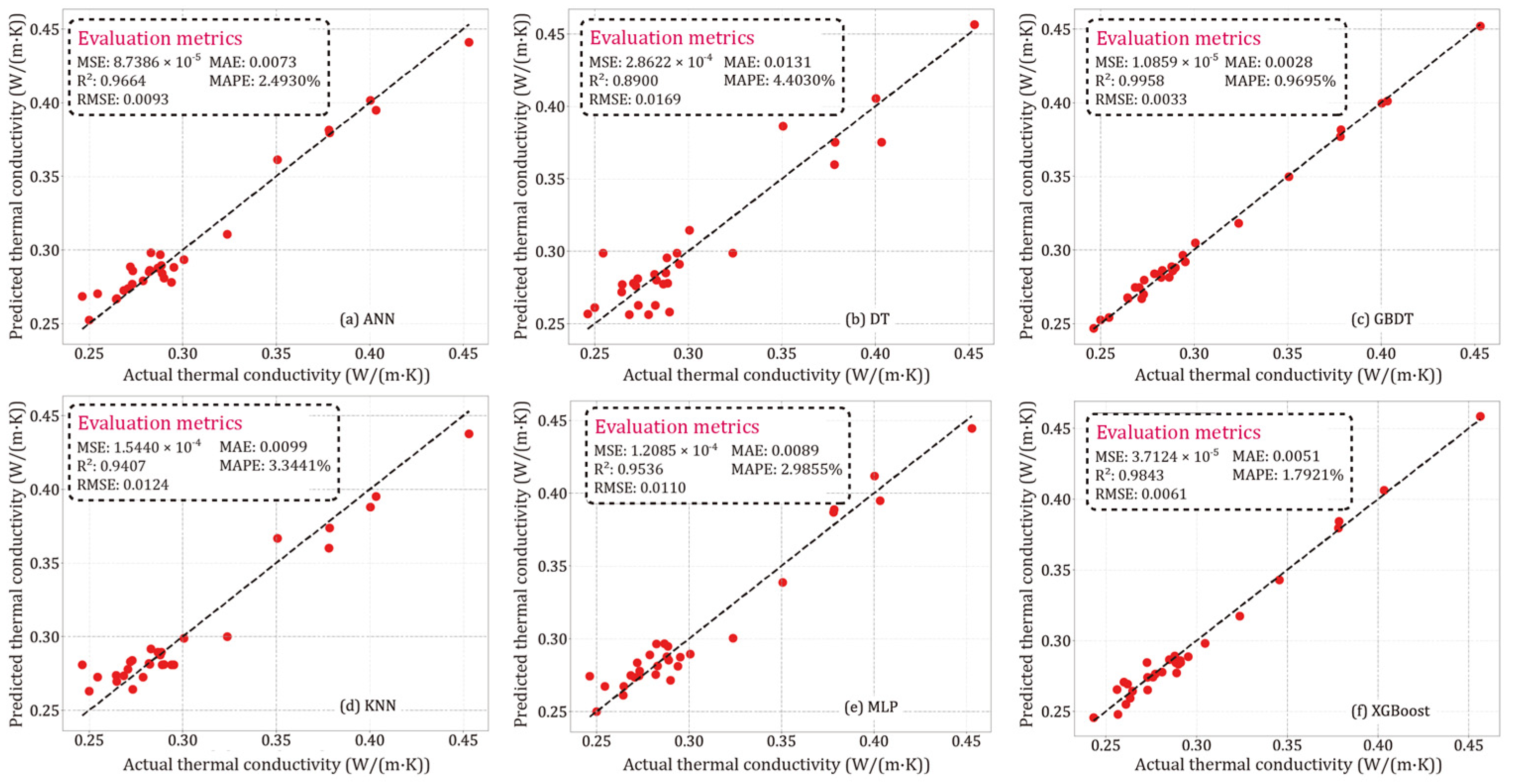
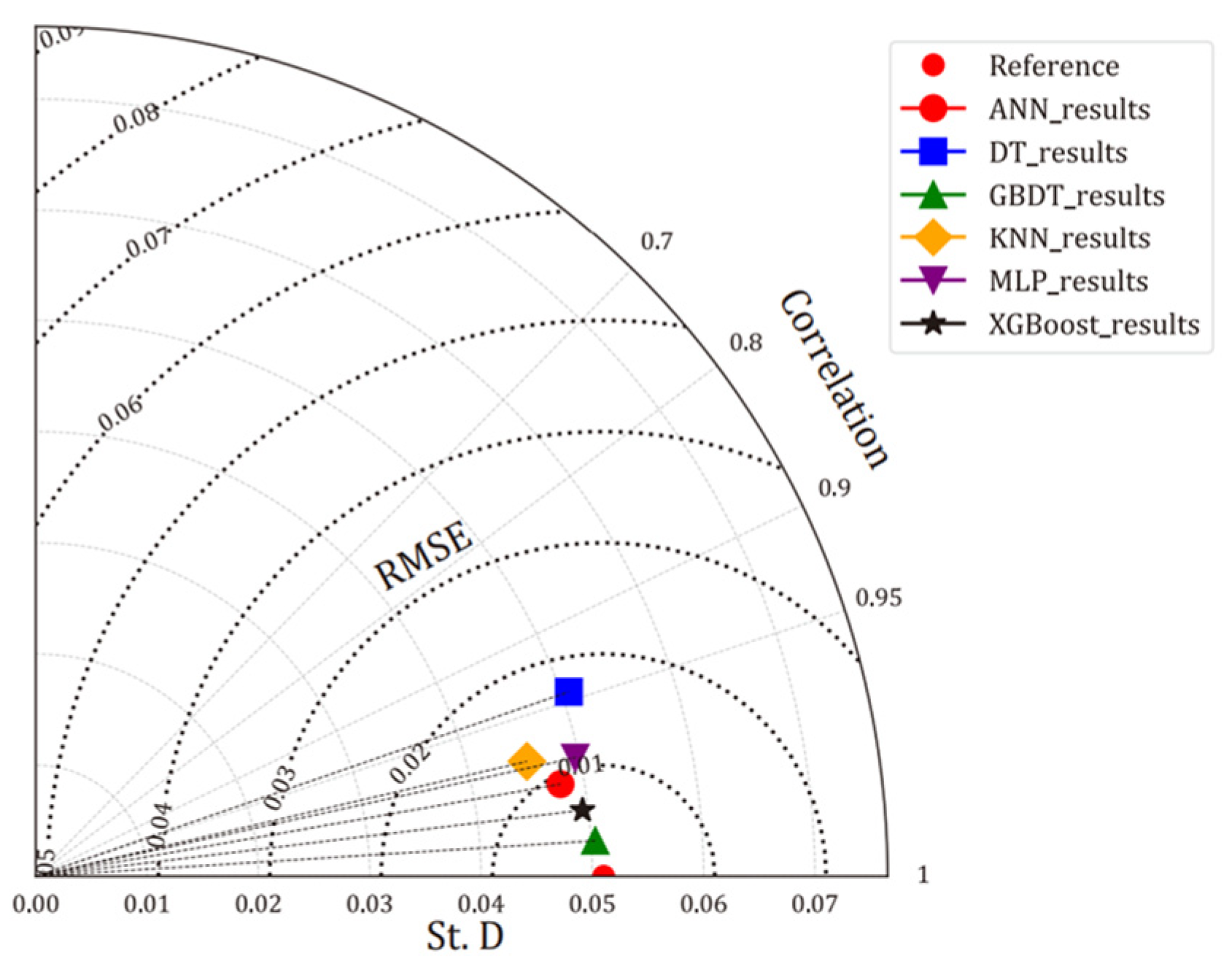
The remainder of this work is organized as follows: Section 2 highlights the significance of this study. Section 3 firstly describes the thermal conductivity of EG–Al₂O₃ nanoparticles, data collection, and feature selection, and then each model is discussed to present its characteristics. Section 4 covers the development of the prediction models. Section 5 presents the results, mainly providing a comparative analysis of model performance in both the training and testing phases, as well as the validation process. The results of parameter sensitivity analysis using SHAP technology is also shown in this section. Finally, Section 6 discusses key findings in this study, practical implications, and future research directions. 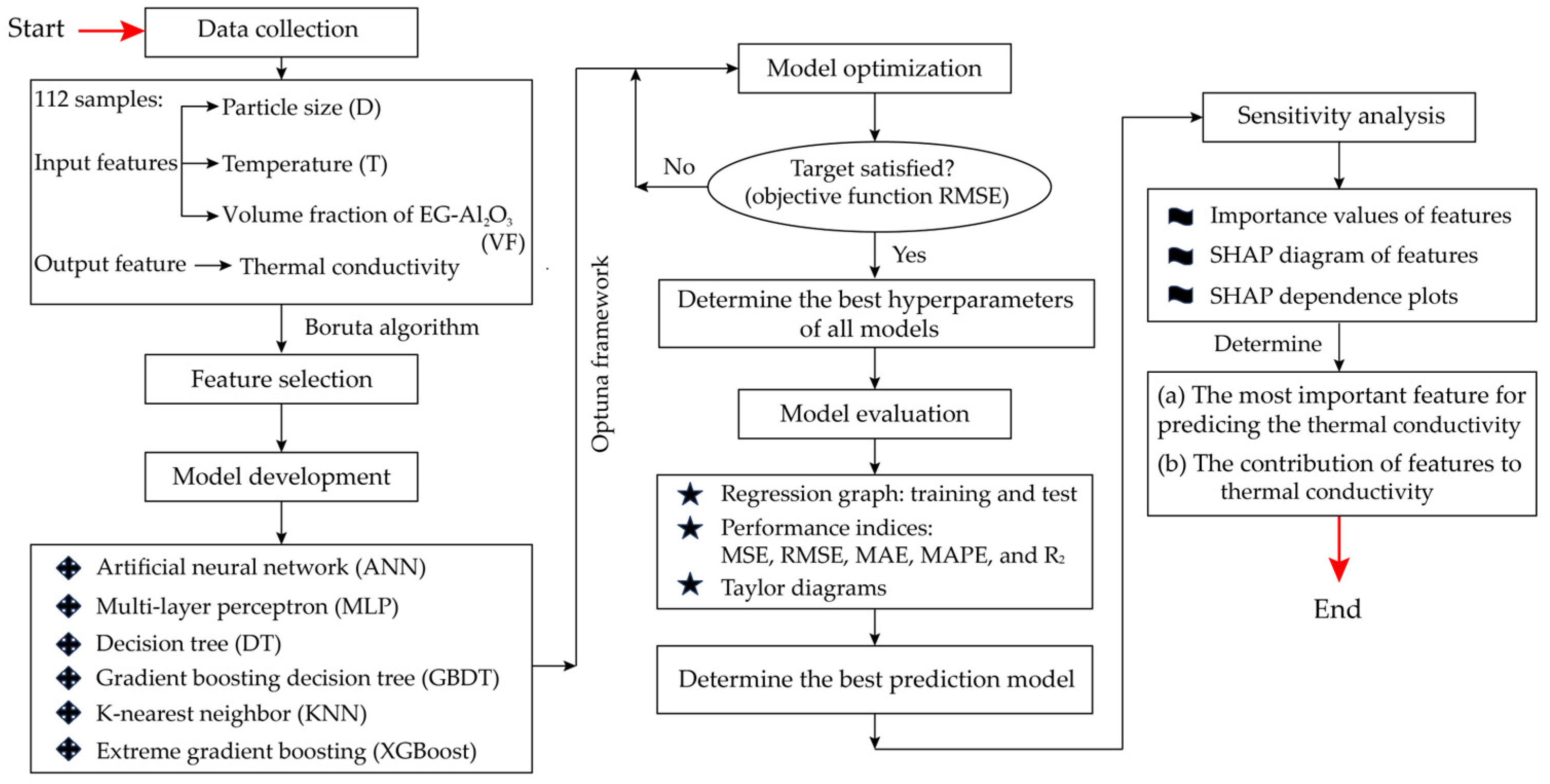The goals and flowchart of this work are shown in Figure 1.

2. Research Significance

Improving the thermal conductivity of EG–Al₂O₃ nanofluids is crucial for heat transfer in cooling systems and heat exchangers. This enhancement allows for more efficient energy use, reduces operational costs, and facilitates the design of more compact systems. Additionally, higher thermal conductivity can expand the range of applications in industries requiring effective thermal management, such as electronics and high-performance engines. The accurate prediction of thermal conductivity in EG–Al₂O₃ nanofluids is pivotal for optimizing energy utilization in various industries, yet it presents significant challenges. Traditional models like those of Maxwell and Hamilton-Crosse have typically simplified complex phenomena such as Brownian motion and particle interactions, leading to significant discrepancies between the predicted and experimental results. This limitation necessitates a shift towards more adaptable and nuanced approaches.

ML models, by virtue of their design, excel in managing complex, nonlinear data interactions without necessitating explicit programmatic formulations of the underlying physical laws. This capability is particularly advantageous in handling the multi-variable nature of nanofluid systems, where factors such as particle size, temperature, and concentration interact in nonlinear ways to affect thermal conductivity. By implementing advanced ML models, this research leverages computational power to derive insights from existing data in a way that is both cost-efficient and robust, offering substantial improvements over conventional methods. This study contributes to the field by: (i) employing six different supervised machine learning models (ANN, DT, GBDT, KNN, MLP, and XGBoost) to predict the thermal conductivity of EG–Al₂O₃ nanofluids, and (ii) utilizing SHAP sensitivity analysis to provide crucial insights that enhance the theoretical understanding and practical application of thermal management in various industries. The six supervised models were developed using four published studies that focused on temperature, particle size, and volume fraction as the primary analytical parameters. These studies were chosen because they provide high-quality and well-organized data.

3. Methodologies

The objective of this study is to enhance the accuracy, reliability, and cost-efficiency of thermal conductivity predictions, overcoming the limitations of traditional theoretical and numerical models. This section begins with a description of the preparation process of the nanofluids, including the synthesis of EG–Al₂O₃ nanoparticles and their stabilization in the base fluid with the aid of surfactants and ultrasonication to ensure a homogenous dispersion. This is followed by an outline of the measurement techniques for thermal conductivity and the use of statistical methods to analyze the data collected from extensive experiments. Subsequently, the focus shifts to the selection of relevant features using the Boruta algorithm, enhancing the predictive accuracy and computational efficiency of the ML models deployed. These models, including ANN, DT, GBDT, KNN, MLP and XGBoost, are each discussed in terms of structure, optimization of hyperparameters, and their specific applications to the dataset.

3.1. Data Preparison

The preparation of Al₂O₃ nanofluids involves several steps to ensure a stable and homogeneous suspension of nanoparticles in the EG base fluid. Al₂O₃ nanoparticles are typically synthesized using methods such as sol–gel [48] and hydrothermal [49] processes. Once synthesized, these nanoparticles are dispersed into the EG base fluid. To prevent the nanoparticles from clumping together, surfactants or dispersants such as sodium dodecyl sulfate (SDS) or polyvinylpyrrolidone (PVP) are added [50], as shown in Figure 2. Finally, ultrasonication is applied to break down any clusters of nanoparticles and ensure their even distribution throughout the fluid [51]. Stability tests, including visual inspection and zeta potential measurements [52], are often conducted to confirm the suspension’s stability over time. Thermal conductivity is then measured using methods such as the transient hotwire method, which involves immersing a thin wire in the nanofluid, passing an electrical current through it, and monitoring the rate of temperature rise [53]. Alternatively, the steady-state parallel-plate method measures the temperature difference and heat flux through the nanofluid between two plates with a known thermal gradient. This study compiled 94 data points from four experimental studies [43,44,45,46], representing nearly all the available research on the thermal conductivity of EG–Al₂O₃ nanofluids, presented in tabular form. These sources were carefully chosen for their consistent research direction and detailed examination of key variables such as particle size, volume fraction, and temperature. This selective approach was taken not only to ensure the coherence and high quality of the data within the database but also to maintain data accuracy and rigor. Non-tabular data sources were deliberately excluded to preserve the precision and integrity of the dataset. The descriptive statistics of this dataset, including measures such as mean, median, standard deviation (St. D), and range, are detailed in

Table 1. Descriptive statics of input and output features.

Features	Sign	Unit	Min	Max	Mean	Median	St. D
Particle size	D	nm	12.00	282.00	30.68	13.00	47.40
Temperature	T	K	283.15	411.10	322.57	308.21	33.84
Volume fraction of EG–Al2O3	VF	vol%	0.00	3.99	1.24	0.80	1.30
Thermal conductivity	/	W/(m·K)	0.24	0.48	0.30	0.29	0.05

.

To enhance the utility of the EG–Al₂O₃ nanofluid dataset for ML applications, it is essential to perform feature selection to identify the most relevant features. By selecting the optimal features, the dataset can be streamlined, resulting in reducing overfitting, improving model accuracy, and decreasing computational costs. The review showed that the Boruta algorithm was one of the most widely used methods to select the reliable features [54]. The operation of the Boruta algorithm can be divided into several steps: (1) Generating a shadow feature dataset by duplication and randomization. During duplication, each original feature is duplicated to create a shadow feature. This means for each original feature, there is a shadow feature. The shadow feature dataset has thus the same dimension as the original dataset. The values in each shadow feature are randomly permuted. This random permutation breaks any association between the shadow feature and the target variable. Essentially, the shadow feature is a shuffled version of the original feature, ensuring it has no predictive power regarding the target variable. The purpose of creating these shadow features is to provide a baseline or reference for evaluating the importance of the original features. If an original feature has higher standard score (Z-Score) than the maximum Z-Score of its shadow feature, this feature is considered as an important factor influencing the target variable. (2) Calculating importance scores (Z-scores) of features belong to the shadow dataset using a prediction model. In this study, the default RF model was used to obtain the maximum feature score. (3) Then, the importance score of each feature within the original dataset is recalculated and compared with the maximum feature score obtained earlier. (4) Finally, all features are classified into two categories: ‘accepted’ means that the importance score of a feature is consistently higher than the maximum feature score; ‘rejected’ means that the importance score of a feature is consistently lower than the maximum feature score. This iterative process continues until all features are decisively accepted or rejected, or until the maximum number of iterations is reached. Figure 3 illustrates the comparison in Z-scores between shadow features (represented by blue boxes) and original features (represented by green boxes). The Z-scores of each feature were calculated 30 times and are presented using quartile statistics: Q1 value (boxplot bottom), median value, Q3 value (boxplot top), and outliers. The analysis revealed that all features had higher Z-scores than the maximum Z-score of the shadow features, indicating that all features were accepted by the Boruta algorithm and could be used to train prediction models in this study.

3.2. Model Description

3.2.1. Artificial Neural Network (ANN)

ANNs are widely used to solve various tasks, including regression, and have powerful ability in learning nonlinear relationships within data, resisting noise interference, and adapting to diverse data [55,56]. A common ANN structure consists of an input layer, one or two hidden layers, and an output layer, as shown in Figure 4. For regression tasks, to minimize errors between the actual and predicted values, the weights need to be adjusted using backpropagation and optimization algorithms such as stochastic gradient descent (SGD), Adam, and limited-memory BFGS (LBFGS) [57,58,59]. Furthermore, regularization techniques are crucial to prevent overfitting; L1 and L2 regularization are commonly used methods. These add a penalty to the loss function based on the absolute values or squared values of the weights, respectively. Thus, the overall objective function ($Obj(\theta )$) for an ANN can be formulated as:

$$\begin{array}{l}Obj(\theta )=L(\theta )+\lambda {\displaystyle \sum _{j=1}^m\left|{\theta }_j\right|} (\mathrm{L}1 \mathrm{regularization})\\ Obj(\theta )=L(\theta )+\lambda {\displaystyle \sum _{j=1}^m{\theta }_j^2} (\mathrm{L}2 \mathrm{regularization})\end{array}$$

(1)

where $L(\theta )$ represents a loss function, $\lambda$ is a regularization parameter, $\left|{\theta }_j\right|$ represents the absolute value of the j-th parameter for L1 regularization, and ${\theta }_j^2$ represents the squared value of the j-th parameter for L2 regularization. m is the number of parameters used in the model. By minimizing this objective function, the model parameters are optimized to achieve a balance between fitting the training data well and maintaining generalizability. In this study, the ANN model’s performance is controlled by several hyperparameters that need to be optimized, including the number of hidden layers (n_layers), the number of neurons in each hidden layer (n_units), the activation function, the solver for the optimization algorithm (a_solver: SGD, Adam, and LBFGS), and the regularization strength (alpha). Note that the common activation functions include the rectified linear unit (ReLU), logistic, and hyperbolic tangent (Tanh) functions.

3.2.2. Multi-Layer Perceptron (MLP)

MLPs consist of an input layer, three or more hidden layers, and an output layer [60]. Each node, except for the input nodes, is a neuron that uses an activation function, as shown in Figure 5. Each neuron in the hidden layers processes the input through weighted connections and an activation function, introducing nonlinearity into the model and enabling it to capture complex patterns. The overall objective function for an MLP structure in regression tasks can be formulated as:

$$Obj(W_1,W_2)=\min \left[{\displaystyle \frac{1}{N}}{\displaystyle \sum _{i=1}^{N}loss(y_i,y_{ture})+\lambda \left({\Vert W_1\Vert }^2+{\Vert W_2\Vert }^2\right)}\right]$$

(2)

where N represents the number of samples, $loss(y_i,y_{ture})$ is the loss between the predicted value $y_i$ and the true value $y_{ture}$, and $W_1$ and $W_2$ are the L2 norms (squared) of the weight matrices for the hidden layers and the output layer, respectively. In this study, eight key hyperparameters optimized include the n_layers, n_units, activation function, a_solver, alpha, batch size (batch_size), initial learning rate (i_learning rate), and maximum iterations (max_iter).

3.2.3. Decision Tree (DT)

DTs are versatile ML algorithms capable of performing both regression and classification tasks. They are advantageous due to their simplicity, interpretability, and ability to handle both numerical and categorical data. The structure of a DT consists of nodes representing feature tests and branches representing outcomes of these tests, culminating in leaf nodes that provide the output predictions. Each node in the tree makes a decision based on the input features, processing them through variance reduction for regression. Thus, the overall objective function for a DT in regression tasks, particularly using the least squares regression tree method, can be formulated as:

$$Obj(j,s)=\min \left[{\displaystyle \sum _{x_i\in R_1(j,s)}{\left(y_{true}-c_1\right)}^2+{\displaystyle \sum _{x_i\in R_2(j,s)}{\left(y_{true}-c_2\right)}^2}}\right]$$

(3)

where $c_1$ is the mean target value in $R_1(j,s)$, and $c_2$ is the mean target value in $R_2(j,s)$. The subsets $R_1(j,s)$ and $R_2(j,s)$ can be the results from the split at the j-th feature with a threshold s. In this study, the key hyperparameters that need to be optimized are listed as follows: the maximum depth of the trees (max_depth), the minimum number of samples required to split an internal node (min_sample_split), and the minimum number of samples required to be at a leaf node (min_sample_leaf). Optimizing these hyperparameters is essential to control the tree’s growth, prevent overfitting, and ensure the model creates meaningful rules from the data without being influenced by noise.

3.2.4. Gradient Boosting Decision Tree (GBDT)

A GBDT is an advanced ensemble learning technique that operates by incrementally building an ensemble of weak decision tree models to form a strong predictive model. The core idea is to compute the residual errors between predicted and actual values, and to use these residuals as targets to train the subsequent tree. As the number of trees increases, the model can be improved by focusing on examples that are hard to predict. This boosting approach leverages the strength of multiple learners to reduce both bias and variance, leading to improved model accuracy and robustness against overfitting. Through iterative minimization of a differentiable loss function, GBDT effectively adapts to various types of predictive modeling tasks, including both regression and classification. A classical GBDT model is shown in Figure 6. The key steps involved when using a GBDT for regression tasks are as follows: (a) initializing with a constant value that minimizes the loss function, iteratively training decision trees on the residual errors of the current model; (b) updating the model by adding the new tree to the existing ensemble, and (c) optimizing the model using gradient descent to minimize the loss function. The advantages of using a GBDT for regression tasks include its accuracy in capturing complex patterns and feature interactions, flexibility in supporting various loss functions for different types of regression problems, and robustness through subsampling and regularization techniques. The objective function for a GBDT in regression tasks can be formulated as:

$$Obj(j,n)=\arg \underset{\gamma }{\min }{\displaystyle \sum _{x_i\in R_{jn}}L\left(y_{true},F_{n-1}\left(x_i\right)+\gamma \right)}$$

(4)

where $F_{n-1}\left(x_i\right)$ is the prediction value at the m − 1-th iterations, $\gamma$ is the optimal adjustment value, and $R_{jn}$ is the region corresponding to the j-th leaf node in the n-th tree. In this study, the GBDT model’s performance is controlled by seven hyperparameters, including the loss function, the number of estimators (n_estimators), the max_depth, the min_sample_split, the min_sample_leaf, the learning rate, and the subsample ratio. Note that four approaches are usually used to generate loss functions of GBDTs, including square error, absolute, Huber, and quantile.

3.2.5. K-Nearest Neighbor (KNN)

KNN predicts the output for a given input by averaging the outputs of its k-nearest neighbors in the feature space. It can model complex relationships in the data without assuming any specific underlying distribution. In this study, the number of neighbors (n_neighbors), the distance metric (p), and the weight function are the main influences on model performance. For instance, the n_neighbors influence the smoothness of the prediction, and p determines how the distance between data points is calculated. Note that two types of weight functions were utilized to improve model performance, i.e., uniform and distance. Obviously, optimizing these hyperparameters is essential to enhance the accuracy and robustness of the model, ensuring that KNN can effectively capture the underlying patterns in the data and provide reliable predictions. The overall objective function for KNN in regression tasks can be formulated as:

$$Obj(y,\partial ,w)=\min \left[{\displaystyle \frac{1}{T}}{{\displaystyle \sum _t^T\left(y_{t,true}-\frac{{\displaystyle \sum _{b\in {\partial }_t}{w}_{tb}{y}_i}}{{\displaystyle \sum _{b\in {\partial }_t}{w}_{tb}}}\right)}}^2\right]$$

(5)

where $y_{t,true}$ is the actual value of the t-th data point, ${\partial }_t$ is the set of neighbors of the t-th data point, $w_{tb}$ is the weight assigned to the neighbor b of the t-th data point, and T represents the total number of data points.

3.2.6. Extreme Gradient Boosting (XGBoost)

XGBoost is a powerful ML algorithm known for its efficiency and performance in predictive modeling tasks. It belongs to the family of boosting algorithms, which build an ensemble of weak learners in a stagewise manner to improve overall prediction accuracy. The hyperparameters of XGBoost are critical in determining model performance. For example, the learning rate controls the contribution of each tree to the final model. The n_estimators determine the number of trees in the ensemble. The max_depth influences the model’s learning ability. Other important hyperparameters include the subsample ratio, the number of features that need to be used before building trees (colsample_bytree), the minimum loss reduction before running the next split (gamma), the L1 regularization term of the weight (reg_alpha), and the L2 regularization term of the weight (reg_lambda). The overall objective function for XGBoost in regression tasks can be formulated as:

$$Obj(i)={\displaystyle \sum _{i}l\left(y_{true},y_{predict}\right)}+{\displaystyle \sum _k\mathsf{\Omega }\left(f_k\right)}$$

(6)

where l() is the loss function measuring the error between the predicted value $y_{predict}$ and the actual value, and $\mathsf{\Omega }$ is the regularization term to control model complexity and prevent overfitting.

4. The Development of the Prediction Models

As demonstrated in Figure 1, the workflow for developing models to predict the thermal conductivity of EG–Al₂O₃ nanofluids can be divided into several parts: data process, hyperparameter optimization, and model evaluation. After that, SHAP analysis is conducted to understand the importance of each feature in the model. This structured workflow ensures a systematic approach to building and evaluating predictive models, leading to more reliable and interpretable outcomes.

(i)

Data process: In this study, 94 data points collected from four published experimental studies are divided into two sub-datasets: (a) the training set and (b) the test set. Generally, the training set contains more data than the test set to validate the model generalization ability. Thus, the data allocation ratio of training set to test set is 7:3, aligning with the number of samples in the training set used in a similar work [61]. To reduce the prediction error caused by the differences in parameter dimensions, all data samples are normalized into the range of 0 to 1.

(ii)

Hyperparameter optimization: The process of hyperparameter optimization is critical to enhance model performance across various indices, including accuracy and efficiency. Inadequate hyperparameter settings can precipitate either underfitting or overfitting, thereby degrading the effectiveness of the model. To that end, the Optuna framework [62] is employed, a Python-based library renowned for its robust and efficient capabilities in hyperparameter optimization. In the optimization process, each trial represents a single evaluation of a set of hyperparameters. The objective is to find the optimal combination of hyperparameters that maximizes the prediction accuracy. The framework of Optuna can be divided into several steps as follows: (a) defining the search space, (b) suggesting hyperparameters, (c) evaluating model performance, (d) updating the search space based on evaluation results, and (e) repeating these steps for a predetermined number of trials or until a stopping criterion is met. To determine the optimal number of iterations and data allocation methods, three versions of the ratio of training set to test set (60:40, 70:30, and 80:20) are used to generate the prediction models through 2000 iterations. The optimization process is executed on a laptop equipped with a 13th Gen Intel(R) Core (TM) i9-13900HX processor (2.20 GHz), 16.0 GB RAM, and an NVIDIA 4060 graphics card. After identifying the optimal number of iterations, the model is reoptimized using the optimal iteration number to determine the best hyperparameters. Furthermore, RMSE is utilized to establish the objective function to evaluate optimization performance. The setting ranges of hyperparameters for the different models are shown in

Table 2. Hyperparameter ranges set in each prediction model.

Models	Hyperparameters
ANN	n_layers: [1, 2]; n_units: [4, 128]; activation function: [‘Relu’, ‘tanh’, ‘logistic’]; a_solver: [‘Adam’, ‘sgd’, ‘lbfgs’]; alpha: [1 × 10−5, 1 × 10−1]
MLP	n_layers: [3, 10]; n_units: [10, 100]; activation function: [‘relu’, ‘tanh’, ‘logistic’, ‘identity’]; a_solver: [‘Adam’, ‘sgd’, ‘lbfgs’]; alpha: [1 × 10−5, 1 × 10−2]; batch_size: [‘auto’, 32, 64, 128]; i_learning rate: [1 × 10−5, 1 × 10−2]; max_iter: [200, 1000]
DT	max_depth: [2, 32]; min_sample_split: [2, 20]; min_sample_leaf: [1, 20]
GBDT	Loss function: [‘square’, ‘absolute’, ‘huber’, ‘quantile’]; n_estimators: [100, 500]; max_depth: [3, 9]; min_sample_split: [2, 10]; min_sample_leaf: [1, 10]; learning rate: [0.01, 0.3]; subsample ratio: [0.5, 1.0]
KNN	n_neighbors: [1, 30]; weight function: [‘uniform’, ‘distance’]; p: [1, 2]
XGBoost	n_estimators: [100, 1000]; max_depth: [3, 10]; learning_rate: [0.01, 0.3]; subsample ratio: [0.5, 1.0]; colsample_bytree: [0.5, 1.0]; gamma: [0.0, 1.0]; reg_alpha: [0.0, 1.0]; reg_lambda: [0.0, 1.0]

.

(iii)

Model evaluation: In this step, several statistical indices, including MSE, RMSE, MAE, MAPE, and R², are adopted to evaluate model performance. These indices provide a comprehensive evaluation of each model’s accuracy and predictive capability. The definitions of these performance indices can be found in the literature [63,64,65,66]. The mathematical expressions of all indices are shown as follows:

$$\mathrm{MSE}={\displaystyle \frac{1}{V}}{{\displaystyle \sum _{v=1}^V\left(y_{true}-y_{predict}\right)}}^2$$

(7)

$$\mathrm{RMSE}=\sqrt{{{\displaystyle \sum _{v=1}^V\left(y_{true}-y_{predict}\right)}}^2}$$

(8)

$$\mathrm{MAE}={\displaystyle \frac{1}{V}}{\displaystyle \sum _{v=1}^V\left|y_{true}-y_{predict}\right|}$$

(9)

$$\mathrm{MAPE}={\displaystyle \frac{1}{V}}{\displaystyle \sum _{v=1}^V\left|\frac{y_{true}-y_{predict}}{y_{true}}\right|}\times 100\%$$

(10)

$${\mathrm{R}}^2=1-{\displaystyle \frac{{{\displaystyle \sum _{v=1}^V\left(y_{true}-y_{predict}\right)}}^2}{{{\displaystyle \sum _{v=1}^V\left(y_{true}-{\overline{y}}_{true}\right)}}^2}}$$

(11)

where V is the number of samples, and ${\overline{y}}_{true}$ is the mean of the actual values. These evaluation indices collectively provide a robust framework for assessing the performance of our models. Analyzing these indices provides insights into the strengths and weaknesses of each model, enabling informed decisions about model selection and optimization. The models are further evaluated using other methods, such as predictive–actual plots and Taylor diagrams. The detailed statement can be found in Section 5.2.

5. Results and Discussion

This section presents the results of the optimization and evaluation of all models developed for predicting the thermal conductivity of EG–Al₂O₃ nanofluids. The analysis covers the optimal iteration times for each model. After that, the performance of each model using the training and test datasets is evaluated to determine the best model. Furthermore, four validation tests are generated to test the robustness of the optimal model across different experimental conditions.

5.1. Iteration Times Optimization for Each Model

The purpose of determining the optimal number of iterations for each model is to find the best compromise between model performance and training cost. This involves analyzing the relationship between the number of iterations and the corresponding fitness values for each model. Figure 7 illustrates the fitness iteration curves during 2000 iterations for six different models: ANN, DT, GBDT, KNN, MLP, and XGBoost. It can be observed that the fitness value (i.e., RMSE value) of each model decreases with more iterations up to a certain count, i.e., the model performance cannot be further improved when the number of iterations exceeds that number. On the other hand, the data allocation method (the ratio of training set to testing set) can significantly influence the model performance, so it is crucial to find the best data configuration. As mentioned earlier, three ratios of training set to test set were validated: 60:40 (blue), 70:30 (red), and 80:20 (black). The 90:10 ratio was excluded in order to retain enough data samples to be able to test model performance. It can be seen that most of the models (ANN, DT, GBDT, KNN, MLP) presented lower RMSE values when the ratio of training set to test set was 70:30. The XGBoost models trained using three allocation methods obtained a similar performance. As a result, the optimal number of iterations for each model can be identified by determining the minimum fitness values based on the best data allocation (the ratio of training set to test set was 70 to 30). The optimal numbers of iterations are: 1400 (ANN), 250 (DT), 1000 (GBDT), 70 (KNN), 350 (MLP), and 800 (XGBoost).

Table 3. Time consumption of each model using three types of data allocation methods.

Models	The Ratio of Training Set to Test Set
	60:40	70:30	80:20
ANN	1231 s	1201 s	2277 s
DT	123 s	115 s	119 s
GBDT	2019 s	823 s	929 s
KNN	89 s	41 s	84 s
MLP	3483 s	4229 s	12,970 s
XGBoost	604 s	380 s	501 s

shows the time consumption of each model and each data allocation method for 2000 iterations. The results indicate that the lowest time consumption among most of the models (ANN, GBDT, KNN and MLP) was obtained by setting the ratio of training set to test set to 70:30. These findings also validate that this ratio of training set to test set is the optimal data allocation used for improving model performance. After determining the optimal number of iterations for each model, all models were retrained to obtain the final hyperparameter values based on the best data allocation. The optimized hyperparameters of each model are summarized in

Table 4. The optimal hyperparameters for each prediction model.

Models	Hyperparameters
ANN	n_layers: [2]; n_units: [123]; activation function: [‘Relu’]; a_solver: [‘lbfgs’]; alpha: [5.3660 × 10−4]
MLP	n_layers: [6]; n_units: [91, 31, 76, 13, 79, 18]; activation function: [‘Relu’]; a_solver: [‘lbfgs’]; alpha: [1.4721 × 10−4]; batch_size: [128]; i_learning rate: [2.0767 × 10−5]; max_iter: [810]
DT	max_depth: [12]; min_sample_split: [2]; min_sample_leaf: [1]
GBDT	Loss function: [‘huber’]; n_estimators: [188]; max_depth: [5]; min_sample_split: [9]; min_sample_leaf: [3]; learning rate: [1.3497 × 10−1]; subsample ratio: [6.8284 × 10−1]
KNN	n_neighbors: [4]; weight function: [‘uniform’]; p: [1]
XGBoost	n_estimators: [100, 1000]; max_depth: [3, 10]; learning_rate: [0.01, 0.3]; subsample ratio: [‘0.5, 1.0]; colsample_bytree: [0.5, 1.0]; gamma: [0.0, 1.0]; reg_alpha: [0.0, 1.0]; reg_lambda: [0.0, 1.0]

. These optimized hyperparameters reflect the best configuration found for each model through the iterative optimization process. As a result, the prediction models with the optimal hyperparameters were used to predict the thermal conductivity of EG–Al₂O₃ nanofluids using the training and test sets.

5.2. Model Performance Evaluation

This section provides a detailed performance evaluation of all ML models using the training and test sets. Firstly, the model performance is illustrated using regression graphs. As shown in Figure 8, the prediction accuracy of each model in the training phase can be illustrated using the distribution of data points. It can be seen that the GBDT, DT, and XGBoost models exhibit a strong correlation between the predicted and actual values, indicating high predictive accuracy. In other words, the points in the above three models are closely aligned along the diagonal line. This alignment suggests that the DT, GBDT, and XGBoost models are effectively capturing the underlying patterns in the training set. In contrast, other models, including ANN, KNN, and MLP, show a greater dispersion of points around the diagonal, reflecting lower prediction accuracy than the DT, GBDT, and XGBoost models. It can be observed that the ANN, KNN, and MLP models exhibit a higher degree of variance and less precision in predicted values. It also means that ANN, KNN, and MLP models may not be as effective in modeling the complex relationships between the input features and predictive targets.

Additionally,

Table 5. Evaluation indices of six models in the training phase.

Models	MSE	RMSE	MAE	R2	MAPE (%)	Score
ANN	5.5044 × 10−4	0.0235	0.0102	0.7872	3.1936	2
DT	4.9854 × 10−7	0.0007	0.0002	0.9998	0.0602	6
GBDT	6.7735 × 10−6	0.0026	0.0009	0.9974	0.2764	4
KNN	8.5289 × 10−4	0.0292	0.0153	0.6703	5.0902	1
MLP	4.5798 × 10−4	0.0214	0.0093	0.8230	2.9757	3
XGBoost	1.8061 × 10−6	0.0013	0.0010	0.9993	0.3283	5

provides a quantitative assessment of each model’s performance on the training set using five evaluation indices, MSE, RMSE, MAE, MAPE, and R², offering detailed insight into each model’s accuracy and reliability. The quantitative results corroborate the visual analysis from Figure 8. It can be observed that the DT, GBDT, and XGBoost models show exceptionally low MSE and RMSE values, along with high R² values close to 1, indicating a perfect prediction in the training phase. In particular, the DT model achieves the best performance represented by all indices, followed by the XGBoost model. The GBDT also performs well but with slightly higher error indices compared to the DT and XGBoost models. On the other hand, the KNN model exhibits the highest MSE, RMSE, MAE, and MAPE values among all models, indicating a poor performance in capturing the underlying data patterns. The ANN and MLP models have similar prediction accuracy but do not reach the levels of the GBDT, DT, and XGBoost models.

While the results obtained earlier provide valuable insights into each model’s performance using the training set, they are not entirely sufficient for a comprehensive evaluation. Thus, the performance of all the developed models must be evaluated using the test set to ensure that the findings generalize well to unseen data. As shown in Figure 9, the KNN and MLP models show higher prediction accuracy in the testing phase than that obtained using the training set. Conversely, a notable decrease in the accuracy of the DT model during the testing phase suggests overfitting to the training phase. To combine the selection decisions from both phases, a ranking score was assigned to further evaluate model performance. Generally, the best model has the highest score among all models. The results listed in

Table 6. Evaluation indices of six models in the testing phase.

Models	MSE	RMSE	MAE	R2	MAPE (%)	Score
ANN	8.7386 × 10−5	0.0093	0.0073	0.9664	2.4930	4
DT	2.8622 × 10−4	0.0169	0.0131	0.8900	4.4030	1
GBDT	1.0859 × 10−5	0.0033	0.0028	0.9958	0.9695	6
KNN	1.5440 × 10−4	0.0124	0.0099	0.9407	3.3441	2
MLP	1.2085 × 10−4	0.0110	0.0089	0.9536	2.9855	3
XGBoost	3.7124 × 10−5	0.0061	0.0051	0.9843	1.7921	5

show that the GBDT model obtained higher scores than the other models for all performance indices. Moreover, considering the ranking scores of all models obtained in the training phase, both the GBDT and XGBoost models achieved the same highest score of 10 among all models. This result shows that these two models have good learning ability and strong applicability. However, the GBDT model needs to be considered the best model overall since it demonstrated superior generalization in the testing phase.

To further compare the predictive performance and agreement among the six ML models for thermal conductivity estimation, an analysis by Taylor diagram is conducted as shown in Figure 10. The Taylor diagram provides a comprehensive visual summary of model performance in terms of correlation, St. D, and RMSE. In the Taylor diagram, the model performance is represented by the distance between the model and the reference. Note that the reference position (red dot) corresponds to the observed data. It can be seen that the GBDT model is close to the reference point, indicating that its prediction performance is higher than the other models. This proximity to the reference point suggests that the GBDT model effectively captures the variability present in the observed data, demonstrating a high level of performance in this aspect. After this model, the XGBoost model also showed a strong performance, though slightly less close to the reference than the GBDT model. This result indicates that the XGBoost model is also a reliable, robust choice for solving prediction tasks relating to the thermal conductivity of EG–Al₂O₃ nanofluids. Both the ANN (red circle), KNN (yellow diamond), and MLP (purple pentagon) models demonstrate moderate capabilities. On the other hand, the DT (blue square) model is positioned further from the reference point. The reason is that the DT model has problems of higher variability and lower correlation, resulting in overfitting issues. Overall, the results in the Taylor diagram confirm that the GBDT was the best model among our six models.

5.3. Model Performance Validation

To further validate the robustness and generalizability of the optimized model, four subsets corresponding to references [43,44,45,46] are used to evaluate the performance of the GBDT model. Figure 11 presents the regression graphs of the GBDT model using different subsets. As shown in Figure 11a, most points are closely clustered around the diagonal, suggesting that the GBDT can effectively capture the relationship between the input features and thermal conductivity. Similarly, the points are well aligned with the diagonal line (see Figure 11b). It means that the GBDT model maintains its high accuracy and reliability. As shown in Figure 11c, there is a modest increase in the dispersion of points around the diagonal, but the GBDT model still performs well overall. This increased dispersion is primarily due to the limited data available in this subset. It can be seen from Figure 11d that the GBDT model also demonstrates a satisfactory performance (MSE: 7.8287 × 10⁻⁶, RMSE: 0.0028; R²: 0.9963, MAE: 0.0017, and MAPE: 0.55%). The points are tightly clustered along the diagonal, reflecting the excellent predictive accuracy of the GBDT model.

To further validate the model generalizability, the best model (i.e., GBDT) is employed to predict a new validation dataset, sourced from a published study [47]. The errors between the predicted and actual values are listed in

Table 7. The results of model validation using a new dataset.

No.	Input Features			Thermal Conductivity (W/(m·K))		Absolute Error
	D (nm)	T (K)	VF (vol%)	Actual	Predicted
1	20	302.0	1.00	0.2580	0.2587	0.0007
2	20	323.4	0.98	0.2590	0.2627	0.0037
3	20	347.3	0.97	0.2620	0.2612	0.0008
4	20	372.2	0.95	0.2670	0.2603	0.0067
5	20	392.4	0.94	0.2640	0.2603	0.0037
6	20	411.1	0.92	0.2600	0.2599	0.0001
7	20	296.3	3.00	0.2760	0.2635	0.0125
8	20	323.6	2.95	0.2820	0.2665	0.0155
9	20	349.0	2.90	0.2840	0.2651	0.0189
10	20	373.3	2.85	0.2850	0.2654	0.0196
11	20	392.1	2.81	0.2870	0.2654	0.0216
12	20	409.6	2.78	0.2800	0.2649	0.0151
13	20	304.0	3.99	0.2900	0.2658	0.0242
14	20	323.7	3.94	0.2910	0.2680	0.0230
15	20	348.5	3.87	0.2940	0.2663	0.0277
16	20	373.3	3.81	0.2930	0.2666	0.0264
17	20	391.0	3.76	0.2880	0.2665	0.0215
18	20	409.0	3.71	0.2850	0.2660	0.0190

. The results illustrate that GBDT exhibits a high degree of accuracy on the validation dataset, with errors predominantly minor and within permissible limits. Specifically, the absolute errors range with a minimum of 0.0001, a maximum of 0.0277, and an average of 0.0145. Overall, the GBDT model can be considered as a reliable and robust model for predicting the thermal conductivity of EG–Al₂O₃ nanofluids in this study.

5.4. Parameter Sensitivity Analysis

To understand the contribution of different features to predictions, feature importance analysis can be conducted using SHAP values [67]. SHAP values quantify the contribution of each feature by considering all possible combinations of features and computing the difference in the model prediction when the feature is included versus when it is not. In this study, the SHAP values are used to show the importance and contribution of each feature to the thermal conductivity of EG–Al₂O₃ nanofluids. Figure 12 presents the feature importance values obtained using SHAP. The bar plot indicates the mean absolute SHAP value for each feature, which represents the importance of features on the output magnitude. The results show that the feature T obtained the highest importance value (0.163) among all features, suggesting it has the most significant influence on the model predictions. After this feature, VF also obtained a higher importance value (0.057) than D (0.023) for predicting the thermal conductivity of EG–Al₂O₃ nanofluids.

Figure 13 provides a detailed SHAP summary plot, depicting the SHAP value for each feature and its impact on the output, with blue indicating low values and red indicating high values. It can be seen that the feature T shows a significant positive contribution to thermal conductivity. This indicates that high temperatures lead to an increase in the thermal conductivity values. Similarly, most SHAP values of VF are positive, which means that this feature has a globally positive impact on the output. As the VF increases, the SHAP values rise, suggesting that high VF enhances the thermal conductivity of the EG–Al₂O₃ nanofluids. In contrast, the feature D exhibits a predominantly negative impact on the output. The SHAP values of D are clustered around negative values, indicating that this feature has a negative impact on the output. In general, this trend demonstrates that while T and VF significantly boost thermal conductivity, D has a minor negative effect on it.

To further analyze the interaction between features and their contribution to the predictions, SHAP dependence plots are employed. These plots illustrate how the SHAP value for each feature varies with the feature value and reveal interactions between features. As shown in Figure 14, the principal feature is represented on the x-axis, while the color indicates the value of the most interacted feature among all features. The y-axis displays the SHAP values calculated for the principal feature. Figure 14a demonstrates the relationship between T and its SHAP values, with the color representing the VF (vol%). It can be observed that all values of T have positive SHAP values, indicating a positive contribution to thermal conductivity. This observation aligns with findings from various studies, suggesting that the enhancement of thermal conductivity with increasing temperature can be attributed to enhanced microconvection driven by Brownian motion [20,68,69]. Figure 14b depicts the SHAP values of VF (vol%) with the color representing D. It is observed that most points have positive SHAP values, indicating a globally positive contribution to the output. However, when VF is less than 0.4% and D equals 13 nm, the SHAP values become negative, indicating a negative contribution to the prediction. For the red points representing a particle size of 13 nm, an increasing trend of SHAP values can be observed until VF reaches 1%, followed by a plateau. Figure 14c illustrates the relationship between D and its SHAP values with the color representing VF (vol%). The SHAP values of D are generally negative, indicating a negative contribution to the prediction, except under specific conditions: D values of 13 nm, 43 nm, and 50 nm when the VF was equal to 0.1%. Overall, these dependence plots provide valuable insights into how different features and their interactions influence the predictions, highlighting the complex relationships within the collected data.

6. Conclusions

This study has evaluated the effectiveness of six supervised ML models in predicting the thermal conductivity of EG–Al₂O₃ nanofluids. A total of 94 experimental data points sourced from four published studies were used to train and test these models. These models were assessed using several performance indices. Additionally, regression analysis and a Taylor diagram were utilized to visually summarize the model performance. The model validation was conducted by re-predicting a subset of each experimental study. Furthermore, SHAP analysis was employed to interpret the models and identify the importance of each feature in the predictions as well as their contribution to the prediction. The main conclusions are as follows:

(a)

The results of the model evaluation indicated that the GBDT model achieved the most satisfactory performance among the six models. In particular, the performance indices obtained by the GBDT model using the training and test sets are both acceptable: MSE of 6.7735 × 10⁻⁶ and 1.0859 × 10⁻⁵, RMSE of 0.0026 and 0.0033, MAE of 0.0009 and 0.0028, R² of 0.9974 and 0.9958, and MAPE of 0.2764% and 0.9695%.

(b)

The sensitivity analysis using SHAP values revealed that T had the highest impact on model prediction, with the highest importance value of 0.16 among all features. The feature importance ranking was determined as T > VF > D. The dependence plots further illustrate that T had a positive contribution to thermal conductivity. In addition, VF had a globally positive contribution to thermal conductivity, but D generally had a negative contribution to thermal conductivity, except under specific conditions such as D values of 13 nm, 43 nm, and 50 nm with a volume fraction of 0.1%.

In summary, the GBDT model proved to be the most effective in predicting the thermal conductivity of EG–Al₂O₃ nanofluids, demonstrating the potential of ML models to outperform traditional theoretical models and numerical simulations. The use of ML models can significantly aid in the development and optimization of thermal management applications. However, a limitation of this study is that all data were sourced from existing literature, which may affect the models’ generalization capability. Future research should focus on collecting more experimental data to enhance the models’ robustness and generalizability. Additionally, exploring more metaheuristic algorithms could further improve the accuracy and reliability of the proposed models.

References

1. Choi, S.U.S.; Singer, D.A.; Wang, H.P. Developments and applications of non-Newtonian flows. ASME Fed. 1995, 66, 99–105. [Google Scholar]
2. Yu, W.; France, D.M.; Routbort, J.L.; Choi, S.U. Review and comparison of nanofluid thermal conductivity and heat transfer enhancements. Heat Transf. Eng. 2008, 29, 432–460. [Google Scholar] [CrossRef]
3. Keblinski, P.; Eastman, J.A.; Cahill, D.G. Nanofluids for thermal transport. Mater. Today 2005, 8, 36–44. [Google Scholar] [CrossRef]
4. Choi, S.; Zhang, Z.G.; Yu, W.; Lockwood, F.; Grulke, E. Anomalous thermal conductivity enhancement in nanotube suspensions. Appl. Phys. Lett. 2001, 79, 2252–2254. [Google Scholar] [CrossRef]
5. Bozorgan, N. Evaluation of Using Al2O3/EG and TiO2/EG nanofluids as coolants in the double-tube heat exchanger. Int. J. Adv. Des. Manuf. Technol. 2012, 5, 27–34. [Google Scholar]
6. Zamzamian, A.; Oskouie, S.N.; Doosthoseini, A.; Joneidi, A.; Pazouki, M. Experimental investigation of forced convective heat transfer coefficient in nanofluids of Al2O3/EG and CuO/EG in a double pipe and plate heat exchangers under turbulent flow. Exp. Therm. Fluid Sci. 2011, 35, 495–502. [Google Scholar] [CrossRef]
7. Chiam, H.; Azmi, W.; Usri, N.; Mamat, R.; Adam, N. Thermal conductivity and viscosity of Al2O3 nanofluids for different based ratio of water and ethylene glycol mixture. Exp. Therm. Fluid Sci. 2017, 81, 420–429. [Google Scholar] [CrossRef]
8. Nguyen, C.T.; Roy, G.; Gauthier, C.; Galanis, N. Heat transfer enhancement using Al2O3–water nanofluid for an electronic liquid cooling system. Appl. Therm. Eng. 2007, 27, 1501–1506. [Google Scholar] [CrossRef]
9. Guo, W.; Li, G.; Zheng, Y.; Dong, C. The effect of flow pulsation on Al2O3 nanofluids heat transfer behavior in a helical coil: A numerical analysis. Chem. Eng. Res. Des. 2020, 156, 76–85. [Google Scholar] [CrossRef]
10. Mukherjee, S.; Chakrabarty, S.; Mishra, P.C.; Chaudhuri, P. Transient heat transfer characteristics and process intensification with Al2O3-water and TiO2-water nanofluids: An experimental investigation. Chem. Eng. Process.-Process Intensif. 2020, 150, 107887. [Google Scholar] [CrossRef]
11. Maxwell, J. A physical treatise on electricity and magnetism. J. Frankl. Inst. 1881, 111, 386–389. [Google Scholar]
12. Hui, P.; Zhang, X.; Markworth, A.; Stroud, D. Thermal conductivity of graded composites: Numerical simulations and an effective medium approximation. J. Mater. Sci. 1999, 34, 5497–5503. [Google Scholar] [CrossRef]
13. Hamilton, R.L.; Crosser, O. Thermal conductivity of heterogeneous two-component systems. Ind. Eng. Chem. Fundam. 1962, 1, 187–191. [Google Scholar] [CrossRef]
14. Xuan, Y.; Li, Q. Heat transfer enhancement of nanofluids. Int. J. Heat Fluid Flow 2000, 21, 58–64. [Google Scholar] [CrossRef]
15. Jang, S.P.; Choi, S.U. Role of Brownian motion in the enhanced thermal conductivity of nanofluids. Appl. Phys. Lett. 2004, 84, 4316–4318. [Google Scholar] [CrossRef]
16. Prasher, R.; Phelan, P.E.; Bhattacharya, P. Effect of aggregation kinetics on the thermal conductivity of nanoscale colloidal solutions (nanofluid). Nano Lett. 2006, 6, 1529–1534. [Google Scholar] [CrossRef]
17. Abbasov, H.F. Determination of nanolayer thickness and effective thermal conductivity of nanofluids. J. Dispers. Sci. Technol. 2019, 40, 594–603. [Google Scholar] [CrossRef]
18. Yu, W.; Choi, S.U.S. The role of interfacial layers in the enhanced thermal conductivity of nanofluids: A renovated Hamilton–Crosser model. J. Nanopart. Res. 2004, 6, 355–361. [Google Scholar] [CrossRef]
19. Vajjha, R.S.; Das, D.K. Experimental determination of thermal conductivity of three nanofluids and development of new correlations. Int. J. Heat Mass Transf. 2009, 52, 4675–4682. [Google Scholar] [CrossRef]
20. Jang, S.P.; Choi, S.U.S. Effects of various parameters on nanofluid thermal conductivity. J. Heat Transf. 2007, 129, 617–623. [Google Scholar] [CrossRef]
21. Guo, S.Z.; Li, Y.; Jiang, J.S.; Xie, H.Q. Nanofluids containing γ-Fe2O3 nanoparticles and their heat transfer enhancements. Nanoscale Res. Lett. 2010, 5, 1222–1227. [Google Scholar] [CrossRef]
22. Sundar, L.S.; Singh, M.K.; Sousa, A.C. Investigation of thermal conductivity and viscosity of Fe3O4 nanofluid for heat transfer applications. Int. Commun. Heat Mass Transf. 2013, 44, 7–14. [Google Scholar] [CrossRef]
23. Khedkar, R.S.; Kiran, A.S.; Sonawane, S.S.; Wasewar, K.; Umre, S.S. Thermo—Physical Characterization of Paraffin based Fe3O4 Nanofluids. Procedia Eng. 2013, 51, 342–346. [Google Scholar] [CrossRef]
24. Yu, W.; Xie, H.; Chen, L.; Li, Y. Enhancement of thermal conductivity of kerosene-based Fe3O4 nanofluids prepared via phase-transfer method. Colloids Surf. A Physicochem. Eng. Asp. 2010, 355, 109–113. [Google Scholar] [CrossRef]
25. Lenin, R.; Joy, P.A. Role of primary and secondary surfactant layers on the thermal conductivity of lauric acid coated magnetite nanofluids. J. Phys. Chem. C 2016, 120, 11640–11651. [Google Scholar] [CrossRef]
26. Lenin, R.; Joy, P.A. Role of base fluid on the thermal conductivity of oleic acid coated magnetite nanofluids. Colloids Surf. A Physicochem. Eng. Asp. 2017, 529, 922–929. [Google Scholar] [CrossRef]
27. Altan, C.L.; Gurten, B.; Sommerdijk, N.A.; Bucak, S. Deterioration in effective thermal conductivity of aqueous magnetic nanofluids. J. Appl. Phys. 2014, 116, 224904. [Google Scholar] [CrossRef]
28. Lenin, R.; Joy, P.A.; Bera, C. A review of the recent progress on thermal conductivity of nanofluid. J. Mol. Liq. 2021, 338, 116929. [Google Scholar] [CrossRef]
29. Sarkar, S.; Selvam, R.P. Molecular dynamics simulation of effective thermal conductivity and study of enhanced thermal transport mechanism in nanofluids. J. Appl. Phys. 2007, 102, 074302. [Google Scholar] [CrossRef]
30. Nazir, U.; Sohail, M.; Singh, A.; Muhsen, S.; Galal, A.M.; Tag El Din, E.S.M.; Hussain, S.M. Finite element analysis for thermal enhancement in power law hybrid nanofluid. Front. Phys. 2022, 10, 996174. [Google Scholar] [CrossRef]
31. Basu, A.; Saha, A.; Banerjee, S.; Roy, P.C.; Kundu, B. A Review of Artificial Intelligence Methods in Predicting Thermophysical Properties of Nanofluids for Heat Transfer Applications. Energies 2024, 17, 1351. [Google Scholar] [CrossRef]
32. Ahmadi, M.H.; Ahmadi, M.A.; Nazari, M.A.; Mahian, O.; Ghasempour, R. A proposed model to predict thermal conductivity ratio of Al2O3/EG nanofluid by applying least squares support vector machine (LSSVM) and genetic algorithm as a connectionist approach. J. Therm. Anal. Calorim. 2019, 135, 271–281. [Google Scholar] [CrossRef]
33. Ahmadloo, E.; Azizi, S. Prediction of thermal conductivity of various nanofluids using artificial neural network. Int. Commun. Heat Mass Transf. 2016, 74, 69–75. [Google Scholar] [CrossRef]
34. Sharma, P.; Ramesh, K.; Parameshwaran, R.; Deshmukh, S.S. Thermal conductivity prediction of titania-water nanofluid: A case study using different machine learning algorithms. Case Stud. Therm. Eng. 2022, 30, 101658. [Google Scholar] [CrossRef]
35. Ganga, S.; Uddin, Z.; Asthana, R.; Hassan, H.; Bhardwaj, A. Modelling of Viscosity and Thermal Conductivity of Water-Based Nanofluids using Machine-Learning Techniques. Int. J. Math. Eng. Manag. Sci. 2023, 8, 817. [Google Scholar] [CrossRef]
36. Khosrojerdi, S.; Vakili, M.; Yahyaei, M.; Kalhor, K. Thermal conductivity modeling of graphene nanoplatelets/deionized water nanofluid by MLP neural network and theoretical modeling using experimental results. Int. Commun. Heat Mass Transf. 2016, 74, 11–17. [Google Scholar] [CrossRef]
37. Said, Z.; Sharma, P.; Bora, B.J.; Pandey, A.K. Sonication impact on thermal conductivity of f-MWCNT nanofluids using XGBoost and Gaussian process regression. J. Taiwan Inst. Chem. Eng. 2023, 145, 104818. [Google Scholar] [CrossRef]
38. Karniadakis, G.E.; Kevrekidis, I.G.; Lu, L.; Perdikaris, P.; Wang, S.; Yang, L. Physics-informed machine learning. Nat. Rev. Phys. 2021, 3, 422–440. [Google Scholar] [CrossRef]
39. Wang, Y.; Ren, Q. A versatile inversion approach for space/temperature/time-related thermal conductivity via deep learning. Int. J. Heat Mass Transf. 2022, 186, 122444. [Google Scholar] [CrossRef]
40. Zhou, J.; Li, R.; Luo, T. Physics-informed neural networks for modeling mesoscale heat transfer using the Boltzmann transport equation. Adv. Heat Transf. 2023, 55, 211–238. [Google Scholar]
41. Li, Z. Extracting spatial effects from machine learning model using local interpretation method: An example of SHAP and XGBoost. Comput. Environ. Urban Syst. 2022, 96, 101845. [Google Scholar] [CrossRef]
42. Kumar, P.; Jayan, K.D.; Sharma, P.; Alruqi, M. Thermo-electro-rheological properties of graphene oxide and MXene hybrid nanofluid for vanadium redox flow battery: Application of explainable ensemble machine learning with hyperparameter optimization. FlatChem 2024, 43, 100606. [Google Scholar] [CrossRef]
43. Pastoriza-Gallego, M.J.; Lugo, L.; Legido, J.L.; Piñeiro, M.M. Thermal conductivity and viscosity measurements of ethylene glycol-based Al2O3 nanofluids. Nanoscale Res. Lett. 2011, 6, 221. [Google Scholar] [CrossRef] [PubMed]
44. Beck, M.P.; Yuan, Y.; Warrier, P.; Teja, A.S. The thermal conductivity of alumina nanofluids in water, ethylene glycol, and ethylene glycol+ water mixtures. J. Nanopart. Res. 2010, 12, 1469–1477. [Google Scholar] [CrossRef]
45. Beck, M.P.; Yuan, Y.; Warrier, P.; Teja, A.S. The effect of particle size on the thermal conductivity of alumina nanofluids. J. Nanopart. Res. 2009, 11, 1129–1136. [Google Scholar] [CrossRef]
46. Krishnakumar, T.S.; Viswanath, S.P.; Varghese, S.M. Experimental studies on thermal and rheological properties of Al2O3–ethylene glycol nanofluid. Int. J. Refrig. 2018, 89, 122–130. [Google Scholar]
47. Beck, M.P.; Sun, T.; Teja, A.S. The thermal conductivity of alumina nanoparticles dispersed in ethylene glycol. Fluid Phase Equilibria 2007, 260, 275–278. [Google Scholar] [CrossRef]
48. Mohammed, A.A.; Khodair, Z.T.; Khadom, A.A. Preparation and investigation of the structural properties of α-Al2O3 nanoparti- cles using the sol-gel method. Chem. Data Collect. 2020, 29, 100531. [Google Scholar] [CrossRef]
49. Noguchi, T.; Matsui, K.; Islam, N.M.; Hakuta, Y.; Hayashi, H. Rapid synthesis of γ-Al2O3 nanoparticles in supercritical water by continuous hydrothermal flow reaction system. J. Supercrit. Fluids 2008, 46, 129–136. [Google Scholar] [CrossRef]
50. Zhai, Y.; Li, L.; Wang, J.; Li, Z. Evaluation of surfactant on stability and thermal performance of Al2O3-ethylene glycol (EG) nanofluids. Powder Technol. 2019, 343, 215–224. [Google Scholar] [CrossRef]
51. Syarif, D.G. Characteristics of ethylene glycol-Al2O3 nanofluids prepared by utilizing Al2O3 nanoparticles synthesized from local bauxite. In Proceedings of the Journal of Physics: Conference Series; IOP Publishing: Bristol, UK, 2016; Volume 776, p. 012042. [Google Scholar]
52. Xu, J.; Bandyopadhyay, K.; Jung, D. Experimental investigation on the correlation between nano-fluid characteristics and thermal properties of Al2O3 nano-particles dispersed in ethylene glycol–water mixture. Int. J. Heat Mass Transf. 2016, 94, 262–268. [Google Scholar] [CrossRef]
53. Assael, M.J.; Antoniadis, K.D.; Velliadou, D.; Wakeham, W.A. Correct use of the transient hot-wire technique for thermal conductivity measurements on fluids. Int. J. Thermophys. 2023, 44, 85. [Google Scholar] [CrossRef]
54. Kursa, M.B.; Rudnicki, W.R. Feature Selection with the Boruta Package. J. Stat. Softw. 2010, 36, 1–13. [Google Scholar] [CrossRef]
55. Tu, J.V. Advantages and disadvantages of using artificial neural networks versus logistic regression for predicting medical outcomes. J. Clin. Epidemiol. 1996, 49, 1225–1231. [Google Scholar] [CrossRef]
56. Mijwel, M.M. Artificial neural networks advantages and disadvantages. Mesopotamian J. Big Data 2021, 2021, 29–31. [Google Scholar] [CrossRef]
57. Bottou, L. Stochastic gradient learning in neural networks. Proc. Neuro-Nımes 1991, 91, 12. [Google Scholar]
58. Diederik, P.K. Adam: A method for stochastic optimization. arXiv 2014, arXiv:1412.6980. [Google Scholar]
59. Yadav, R.K. PSO-GA based hybrid with Adam Optimization for ANN training with application in Medical Diagnosis. Cogn. Syst. Res. 2020, 64, 191–199. [Google Scholar] [CrossRef]
60. Hounmenou, C.G.; Gneyou, K.E.; Kakaï, R.L.G. A formalism of the general mathematical expression of multilayer perceptron neural networks. Preprints 2021, 2021050412. [Google Scholar]
61. Li, L.; Zhai, Y.; Jin, Y.; Wang, J.; Wang, H.; Ma, M. Stability, thermal performance and artificial neural network modeling of viscosity and thermal conductivity of Al2O3-ethylene glycol nanofluids. Powder Technol. 2020, 363, 360–368. [Google Scholar] [CrossRef]
62. Akiba, T.; Sano, S.; Yanase, T.; Ohta, T.; Koyama, M. Optuna: A Next-generation Hyperparameter Optimization Framework. In Proceedings of the 25th ACM SIGKDD International Conference on Knowledge Discovery and Data Mining, Anchorage, AK, USA, 4–8 August 2019. [Google Scholar]
63. Zhou, J.; Chen, Y.; Li, C.; Qiu, Y.; Huang, S.; Tao, M. Machine learning models to predict the tunnel wall convergence. Transp. Geotech. 2023, 41, 101022. [Google Scholar] [CrossRef]
64. Mei, X.; Cui, Z.; Sheng, Q.; Zhou, J.; Li, C. Application of the improved POA-RF model in predicting the strength and energy absorption property of a novel aseismic rubber-concrete material. Materials 2023, 16, 1286. [Google Scholar] [CrossRef] [PubMed]
65. Li, C.; Zhou, J.; Du, K.; Armaghani, D.J.; Huang, S. Prediction of flyrock distance in surface mining using a novel hybrid model of harris hawks optimization with multi-strategies-based support vector regression. Nat. Resour. Res. 2023, 32, 2995–3023. [Google Scholar] [CrossRef]
66. Li, C.; Zhou, J.; Armaghani, D.J.; Li, X. Stability analysis of underground mine hard rock pillars via combination of finite difference methods, neural networks, and Monte Carlo simulation techniques. Undergr. Space 2021, 6, 379–395. [Google Scholar] [CrossRef]
67. Shapley, L.S. A value for n-person games. In Contributions to the Theory of Games (AM-28); Princeton University Press: Princeton, NJ, USA, 2016; Volume 17, pp. 307–318. [Google Scholar] [CrossRef]
68. Patel, H.E.; Das, S.K.; Sundararajan, T.; Sreekumaran Nair, A.; George, B.; Pradeep, T. Thermal conductivities of naked and monolayer protected metal nanoparticle based nanofluids: Manifestation of anomalous enhancement and chemical effects. Appl. Phys. Lett. 2003, 83, 2931–2933. [Google Scholar] [CrossRef]
69. Das, S.K.; Putra, N.; Thiesen, P.; Roetzel, W. Temperature dependence of thermal conductivity enhancement for nanofluids. J. Heat Transf. 2003, 125, 567–574. [Google Scholar] [CrossRef]
Figure 1. Illustration of a workflow for predictions of the thermal conductivity of EG–Al2O3 nanofluids.
Applsci 14 06264 g001
Figure 2. EG–Al2O3 nanofluid preparation process, thermal conductivity measurement, and application fields.
Applsci 14 06264 g002
Figure 3. Feature selection based on the Boruta algorithm.
Applsci 14 06264 g003
Figure 4. Illustration of ANN model used to predict the thermal conductivity of EG–Al2O3 nanofluids.
Applsci 14 06264 g004
Figure 5. Illustration of MLP model used to predict the thermal conductivity of EG–Al2O3 nanofluids.
Applsci 14 06264 g005
Figure 6. Illustration of GBDT building process by adding weak learners.
Applsci 14 06264 g006
Figure 7. Iteration plots for various prediction models: (a) ANN; (b) DT; (c) GBDT; (d) KNN; (e) MLP; (f) XGBoost.
Applsci 14 06264 g007
Figure 8. Regression graphs of six prediction models using the training set: (a) ANN; (b) DT; (c) GBDT; (d) KNN; (e) MLP; (f) XGboost.
Applsci 14 06264 g008
Figure 9. Regression graphs of six prediction models using the testing set: (a) ANN; (b) DT; (c) GBDT; (d) KNN; (e) MLP; (f) XGboost.
Applsci 14 06264 g009
Figure 10. Taylor diagram of all ML models in the testing phase.
Applsci 14 06264 g010
Figure 11. Regression graphs of the optimal models using four subsets: (a) [43]; (b) [44]; (c) [45]; (d) [46].
Applsci 14 06264 g011
Figure 12. Importance values of features through SHAP analysis.
Applsci 14 06264 g012
Figure 13. SHAP diagram of features through SHAP analysis.
Applsci 14 06264 g013
Figure 14. (ac) SHAP dependence plots of T, VF, and D based on the optimal model.
Applsci 14 06264 g014