Prediction of Accident Risk Levels in Traffic Accidents Using Deep Learning and Radial Basis Function Neural Networks Applied to a Dataset with Information on Driving Events

Abstract

A complex AI system must be worked offline because the training and execution phases are processed separately. This process often requires different computer resources due to the high model requirements. A limitation of this approach is the convoluted training process that needs to be repeated to obtain models with new data continuously incorporated into the knowledge base. Although the environment may be not static, it is crucial to dynamically train models by integrating new information during execution. In this article, artificial neural networks (ANNs) are developed to predict risk levels in traffic accidents with relatively simpler configurations than a deep learning (DL) model, which is more computationally intensive. The objective is to demonstrate that efficient, fast, and comparable results can be obtained using simple architectures such as that offered by the Radial Basis Function neural network (RBFNN). This work led to the generation of a driving dataset, which was subsequently validated for testing ANN models. The driving dataset simulated the dynamic approach by adding new data to the training on-the-fly, given the constant changes in the drivers’ data, vehicle information, environmental conditions, and traffic accidents. This study compares the processing time and performance of a Convolutional Neural Network (CNN), Random Forest (RF), Radial Basis Function (RBF), and Multilayer Perceptron (MLP), using evaluation metrics of accuracy, Specificity, and Sensitivity-recall to recommend an appropriate, simple, and fast ANN architecture that can be implemented in a secure alert traffic system that uses encrypted data.

1. Introduction

Road traffic deaths and injuries continue to pose a significant challenge to global health and development. According to the WHO’s Global Status Report on Road Safety 2023 [1], road traffic crashes are the leading cause of death among children and adolescents aged 5 to 29 years. In 2021, an estimated 1.19 million people died due to road traffic accidents, which is a 5% decrease from the 1.25 million deaths recorded in 2010. Even with the global motor vehicle fleet doubling, there has been a slight overall reduction in deaths. Despite this, the cost of mobility remains excessively high. Nine out of ten deaths occur in low- and middle-income countries, while individuals in low-income countries continue to face the highest risk of death per capita.

In 2023, the Ecuadorian National Transit Agency (ANT) recorded 20,994 traffic accidents nationwide. Of these, 20.78% involved cars alone, resulting in 18,605 injuries and 2373 fatalities. Among cities with the largest populations, Guayaquil had the highest traffic accidents, with 4402, followed by Quito, with 3816 accidents [2].

These facts motivated the search for practical solutions to prevent more lives from being lost due to traffic accidents. An interesting proposal, mentioned by Ren et al. [3], is to use the large flow of traffic data that can be obtained and, through the use of DL and ANNs, develop predictive models to reduce the risk levels of traffic accidents, which can be implemented in effective risk warning systems for drivers. However, it is important to note that obtaining good prediction accuracy of the risk of traffic accidents is complicated because it is related to several factors [4], like weather and road conditions, which affect the effectiveness. Another reason is that various conditions differ from one region to another. Tritat and Lee [5] mentioned that predicting traffic accident risk remains challenging due to many factors contributing to accidents, including the number of vehicles on the road and external conditions like weather, road conditions, ambient lighting, and time of day. They also indicated that recent studies have attempted to combine various factors using complex models to make better and more precise predictions.

ML methods have been extensively utilized in traffic prediction problems, allowing for the prediction of multiple crash injuries using data that include different causes and factors from events on roads and streets [6]. Several studies [7,8] have explored and analyzed various types of ANNs and concluded that the Multilayer Perceptron neural network (MLPNN) is the most commonly used ANN for predicting road accidents. They also found that, in some cases, the RBFNN has better predictive performance than the MLPNN, but this difference could be due to several factors. However, Ye et al. [9] state that predicting traffic accident risk requires a lot of data. Therefore, many researchers have turned to DL to develop models for accident risk analysis. Modern DL networks usually consist of tens or hundreds of successive layers to discover complex structures in high-dimensional data and to extract hierarchical representations in feature learning [10]. Tian and Zhang [11] mentioned that DL has been called the technology that will change the world and affirm that Recurrent Neural Networks (RNNs) and CNNs are the most widely used DL models. The continuous development of DL has led many researchers to adopt this technology for building risk evaluation models [9]. Long Short-Term Memory (LSTM) is also applied to many diverse learning problems that differ significantly in their scale and nature from the initially tested problems [12]. An LSTM model can store previous data and predict future risk trends, making it widely applicable in risk forecasting.

It is crucial to note that the RBFNN is part of the conventional Feed-Forward Network (FFN) variety [13], which is a universal approximation function. It is worth mentioning that RBF has greater precision in describing the relationships between risk factors and accident frequency. Moreover, the network structure, primarily denoting the number of nodes in hidden and input layers, is a crucial aspect of neural network model development, given its significant impact on generalization performance. The RBFNN proved to have a significant advantage in approximating, classifying, and speeding up processes [14].

This study aims to prove that RBFNN learning is faster than DL when only three levels (an input, hidden layer, and output layer) are applied. This allows for a dynamic dataset to be used under changing conditions and for faster validation to obtain new prediction models. Moreover, predictions made using the RBFNN are easily auditable, and the results can be comparable to those achieved with DL. A key objective of this work is to demonstrate that efficient, fast, and comparable results can be obtained using simple architectures, such as the RBFNN, by comparing and evaluating these approaches in traffic accident risk-level prediction and the implications of using a dynamic dataset. We use the term dynamic dataset [15] to refer to a process that incorporates new data of driving characteristics collected at specific time intervals from vehicle agents, processed using relevant mechanisms and algorithms, and finally added to the main dataset, making the process continuously changed. This driving dataset was developed due to this research, and its effectiveness was proven by implementing the models presented in this work.

This work follows the structure outlined below: Section 2 analyzes related work, Section 3 presents the materials and methods used, Section 4 compares the model’s results, Section 5 presents the discussion, and Section 6 shows the conclusions.

2. Related Work

Building an effective traffic accident risk prediction system is important in traffic accident prevention. However, predicting the risk of a traffic accident is difficult because many related factors are involved [3]. For that reason, several types of research have been developed to predict the risk of traffic accidents.

Table 1. Comparative table of related work.

Authors	Neural Networks	Purpose	Accuracy/Results	Predicted Classes
Agarwal [16]	CNN	Develop a machine learning approach using a CNN for predicting accident risk.	Precision: 93%, Recall: 94%, F1-score: 0.86	2
Kumeda et al. [17]	Fuzzy-FARCHD, RBFNN, RF, NB, MLPNN	Compare different classifier algorithms using a dataset of crash injury categories.	Accuracy: Fuzzy-FARCHD 85.94%, RBFNN 84.14%, RF 83.42%, NB 80.90%, MLPNN 79.27%	3
Moosavic et al. [18]	DAP (LSTM)	Propose a deep neural network model called the DAP to predict the risk of a traffic incident.	F1-score: 0.65	2
Zhao et al. [19]	CNN, RF	Propose a traffic accident risk forecasting algorithm based on deep learning for edge-cloud internet of vehicles.	AUC: 0.9921	2
Huang et al. [20]	CNN	Investigate the feasibility of utilizing deep learning models to identify and forecast crash occurrence.	Accuracy: 77.34%, F1-score: 0.7651	2
Lee et al. [21]	RF, FFNN	Develop a risk-level accident classifier using a deep learning method to predict high-risk taxi drivers.	Accuracy: 86%, F1-score: 0.77	3
Li et al. [22]	LSTM, CNN	Propose a real-time crash risk prediction model for arterials using LSTM and a CNN.	Sensitivity: LSTM 80%, CNN: 64%, LSTM-CNN 88%	2
Wang et al. [23]	RBF, RF, DFNN-model	Propose a model to predict the levels of risk for traffic accidents.	Accuracy: RBF 71.8%, RF 73.2%, DFNN-model 83%	3
Purkrábková et al. [24]	MLPNN, RF	Conduct a study on the classification of traffic accident risk in urban areas. Their objective was to propose effective traffic management solutions to minimize social losses in cities with high traffic volume.	Accuracy: MLPNN 89%, RF 75.4%	4
Brühwiler et al. [25]	LR, RF, XGBoost, FFNN, LSTM	Evaluate machine learning risk assessment models: LR, RF, XGBoost, FFNN, and LSTM networks.	Accuracy: LR 75.2%, RF 75.7%, XGBoost 75.5%, FFNN 75.4%, LSTM 55.3%	2
Lin et al. [26]	DNN, DBN, MLP, CNN	Develop a model to predict high-risk intersections for traffic accidents.	Accuracy: DNN 72.62%, DBN 72.62%, MLP 71.94%, CNN 72.62%	3
Wang et al. [27]	RF, XGBoost, SVM	Develop prediction models for traffic crash risk potential using traffic-related data.	Accuracy: RF 80%, XGBoost 80%, SVM 81%	3
Kaffash et al. [28]	GRNN (FFNN and RBFNN) and SOM	Present a hybrid predictive model for estimating the risk of road accidents.	Accuracy: 90.74%	2
Park and Hong [29]	MLP	Propose a risk prediction MLP model that reflects the road’s static and dynamic features: length, speed limit, traffic volume, altitude, and azimuth of the sun.	Accuracy: 75%, Precision: 73%, Recall: 81%	4
Amorim et al. [30]	SVM, RF, XGBClassiffer, MLPNN	Conduct experiments with various machine learning algorithms to determine the best classifier for identifying severe or non-severe accident risks associated with Brazilian federal road hotspots.	Accuracy: SVM 58.60%, RF 70.12%, XGBClassiffer 71.25%, MLPNN 83%	2
Jin and Noh [31]	SVM, LR, MLP, CNN-DNN	Propose a system based on deep learning to predict traffic accidents in urban environments and estimate the associated risk levels.	Accuracy: SVM 90%, LR 88%, MLP 90%, CNN-DNN 94%	4

shows an overview of the analyzed related work.

The related works propose approaches that use either a static dataset or a heterogeneous source dataset. However, these studies do not incorporate new data on the fly to train or test new models. Additionally, most of these works do not present the time used for execution and obtaining results.

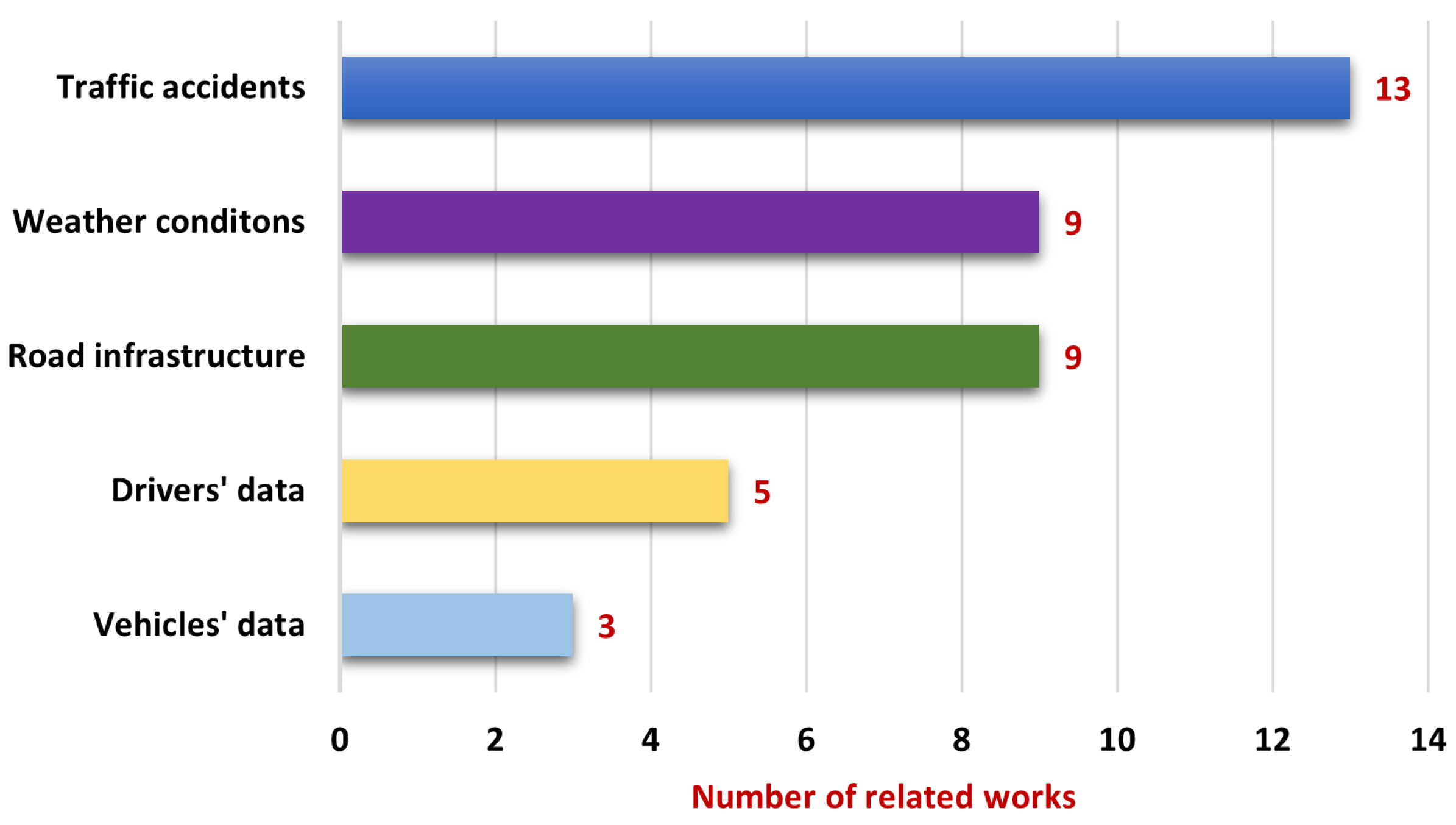
The primary data sources used in the related work were traffic accidents, weather conditions, road infrastructure, drivers’ data, and vehicles’ data. Traffic accidents are the most commonly used data source for estimating the negative effects of traffic incidents. These data include the number of fatalities, injuries, and collisions resulting in casualties or fatalities. It should be noted that the number of attributes used varied from 6 to 42. Figure 1 presents the related work using the most common data sources.

The ANNs and classification algorithms most frequently used in the related work were RF and MLPNN, followed by CNN, RBFNN, and LSTM. These are the most commonly used approaches for developing models that predict the risk of traffic accidents. Figure 2 presents the distribution of the used models in the related work analyzed.

The analyzed studies also showed that CNN and MLPNN achieved the highest accuracy of 93% and 90%, respectively, while RBFNN, RF, and LSTM achieved an accuracy of 84.14%, 83.42%, and 65%, respectively. This evidence suggests that CNN and MLPNN perform better than other ANNs in predicting risk traffic accidents. Figure 3 displays the accuracy of all models used in the related work.

Half of the models in the related work used binary classification, while the other half used multiclass classification; it is important to note that the binary classification models yielded better results than the multiclass classification models. The accuracy may decrease when the number of predictor classes increases. Figure 4 depicts the relationship between the type of classification and the accuracy obtained in the related work.

This study aimed to find an algorithm configuration that reduces the time required for validation and processing when working with this dataset type. Therefore, it was necessary to develop DL networks using CNNs and RFs. A previous study [19] showed that these approaches have achieved the best performance and accuracy in predicting accident risk levels. The performance of all models, including MLPNNs, should be compared to affirm if RBF networks can achieve similar or better results than other networks.

3. Materials and Methods

This investigation is part of a larger project that aims to construct a dataset gathering information on drivers’ data, vehicles’ data, environmental conditions, and traffic accidents in various locations throughout Quito city and its surroundings. By utilizing DL and ML algorithms, the researchers hope to obtain models to assess the risk level of traffic accidents and integrate them into a secure alert system that allows drivers to receive notifications about their current situation via their mobile phones.

The larger project comprises three phases, or agents: acquisition/storage, processing, and presentation. The acquisition/storage agent comprises a mobile application and an OBD2 scanner. Its purpose is to collect information about weather conditions, traffic accident data, and vital sign information of drivers and store all these data in a repository. The processing agent consists of software tools that enable the reading of available driving data, processing it in a machine learning model, and reorganizing the resulting data in a repository. The response or presentation agent is a mobile application that enables the querying of data available from a repository and presenting this information to end users, who represent the drivers that will use this application. Figure 5 displays the complete context of the project mentioned above.

This work contributes to the processing phase by developing and evaluating models through the developed dataset based on various sources, including drivers’ data, weather conditions, traffic accidents, and vehicles’ data, to predict traffic accident risk levels.

3.1. Proposed Models

Four approaches were analyzed to build models and evaluate their performance in classifying accident risk levels. Based on the evidence presented in the related work analyzed in this study, CNN, RF, RBF, and MLP networks were chosen. The results showed that CNNs have a high accuracy rate [19] and good prediction estimates [16], while CNNs, RFs [17], and MLP [31] are the most commonly used networks due to their good performance.

This study aimed to compare the prediction results of CNNs, RFs, and MLP against RBF networks to confirm the quality of RBF in terms of speed and performance prediction. The time required by these models and algorithms to validate and process the acquisition of new models will be the crucial point of comparison because we intend to use a dynamic dataset. The driving dataset must be constantly fed with information, requiring the model to readapt and adjust its parameters to obtain new predictive models. Therefore, the model must be both fast and efficient. The primary contribution of this study is to demonstrate that comparable and fast results can be obtained using simple architectures.

3.2. Deep Learning

ML includes several approaches, in which DL is primarily based on ANNs, designed to simulate the functioning of the human brain [32]. DL represents a new line of research in the field of ML [33]. It is an algorithm that has achieved good results and solves complex problems in pattern recognition. DL has enabled machines to imitate various human activities. For this reason, many researchers [5,9] have chosen this approach to develop risk assessment models.

3.3. Rectified Linear Unit

Rectified Linear Unit (ReLU) is a widely used activation function that adds non-linearity to DL models and resolves the vanishing gradients problem [19]. It ranks among the most commonly used activation functions in DL.

3.4. Convolutional Neural Networks

CNNs are utilized for computer vision and classification tasks [7]. A CNN comprises four main operations: convolution, pooling or subsampling, non-linearity, and classification. The purpose of the convolution layer is to convolve the input features and include a bias [19]. The calculation of the convolutional layer is shown in Equation (1):

$$S(i,j)=(X·W)(i,j)=\sum _m\sum _{n}x(i+m,j+n)·w(m,n)+b,$$

(1)

where X is the input feature, W is the convolutional kernel, and b is the bias.

Recently, Graph Convolutional Networks have emerged as a subject of intense research interest, with their applications extending to image-based depth estimation methodologies. The rationale behind this approach is to use images for classification purposes and to map complex systems into a graph-based representation [34].

3.5. Random Forest

The RF algorithm is a simple ML classification method that can produce accurate results without complicated hyperparameter tuning [17]. It is a tree-based model that can be applied to non-linear classification [27] and regression problems in ML systems.

The RF classifier utilizes the Gini Index (GI) metric for attribute selection [30]. This index measures the impurity of an attribute concerning classes. When selecting a case x randomly from a given training set A and indicating that it belongs to a certain class $C_i$, the $GI$ is defined in (2):

$$\sum \sum _{j\ne i}(f(C_i,A)/\left|A\right|\left)\right(f(C_j,A)/\left|A\right|),$$

(2)

where $f(C_i,A)/\left|A\right|$ represents the probability that the selected case x belongs to class $C_i$.

3.6. Radial Basis Function

The RBFNN is a type of FFNN [35]. It has a simple structure comprising three layers, including a single hidden layer [36]. Its concise training and rapid convergence enable it to approximate any non-linear function [14]. The RBFNN is known for improved prediction efficiency and more stable results [14]. Furthermore, RBFNN frequently demonstrates superior training speeds compared to back-propagation networks [8]. The Gaussian function is considered the basis function of the RBFNN. The representation of the RBFNN output is described in Equation (3):

$$y\left(x\right)=\sum _{i=1}^M{w}_i{e}^{\left({\displaystyle \frac{-{\left(\left|\right|x-c_i\left|\right|\right)}^2}{2{\sigma }^2}}\right)},$$

(3)

where the input, output, center, width, and number of basis functions centered at $c_i$ are denoted by x, $y\left(x\right)$, $c_i$, $\sigma$, and M, respectively. Similarly, weights are denoted by $w_i$.

3.7. Multilayer Perceptron

An MLPNN is a type of FFNN consisting of an input layer, a hidden layer, and an output layer [17]. The most commonly used technique for solving non-linear problems today is with an MLPNN [8].

3.8. Dataset

The PoliDriving dataset was generated with the support of this study. It comprises 2634 samples with 23 numerical features and 1 predictive class; its fields correspond to driver information, vehicle data, weather conditions, and traffic accidents. The data were acquired, processed, and updated to provide a dynamic dataset that supported the development, training, and testing of all obtained models.

During the dataset analysis, it was necessary to perform feature selection to obtain an optimal set of features. The Pearson correlation coefficient, a statistical measure commonly employed by some authors [9,22,37], was used to observe the feature dependencies. It quantifies the degree of linear correlation between two variables, ranging from −1 to 1. The Pearson coefficient reflects the strength of the variables’ relationship.

Finally, we considered the 12 most important features. The significance of these characteristics lies in their ability to encompass a wide range of factors that impact accident risk prediction and their correlation with the target class.

Table 2. Description of the features of the used dataset.

Source	Features	Description	Unit
Driver information	heart_rate	Number of contractions of the heart per minute.	bpm
Vehicle data	steering_angle	Vehicle steering wheel plane angle with respect to the road surface in sexagesimal degrees.	grades
	speed	Vehicle speed in meters per second.	m/s
	rpm	Vehicle engine speed in revolutions per minute.	rpm
	throttle_position	Sensor used to monitor the air intake of the engine.	%
	engine_temperature	Temperature of the air entering the engine.	°C
	system_voltage	Voltage of the vehicle’s electrical system.	V
	distance_travelled	Distance travelled by the vehicle in one-time unit.	km
Weather conditions	latitude	Latitude coordinates of the geographic position.	$\lambda$ degrees
	longitude	Longitude coordinates of the geographic position.	$\omega$ degrees
	barometric_pressure	Pressure variable to change based on weather conditions.	kPa
Traffic accidents	accidents_onsite	Number of deaths due to in accidents at the location.	deaths

describes the selected features of this dataset, and Figure 6 displays the relationship of the features.

The dataset presented another problem: imbalanced data in the predictor class. Imbalanced data significantly affect the learning process since most standard machine learning algorithms expect a balanced class distribution or an equal misclassification cost [38]. For this reason, it was necessary to solve the dataset imbalance problem.

For preprocessing the data, the undersampling technique was used to reduce the number of samples in the minority class to generate a balanced dataset. It was implemented utilizing imbalanced-learn [38], an open-source Python toolkit that offers a broad array of methods for dealing with the common issue of imbalanced datasets in pattern recognition and ML. Thus, the Nearmiss method version 1 [39] was employed to undersample the data. Its objective is to choose a sample from the majority class nearest to multiple samples from the minority class. The selection criterion for samples from the majority class is the one with the smallest average distance to the three nearest samples from the minority class. Using this method, we transformed the unbalanced data into four balanced classes, each with 182 samples. These four predictor classes represent different risk levels: low, medium, high, and extreme.

3.9. Evaluation Metrics

Finally, 5-fold cross-validation was used to estimate the classification model’s skill. One way to evaluate machine learning models is through measurements. These measurements, commonly called evaluation metrics, allow us to measure certain aspects, trends, and results. Thus, for classification problems, the most common metrics are the Prediction Accuracy Rate (PAR), True-Positive Rate (TPR), Sensitivity, True-Negative Rate (TNR), Specificity, F1-score, and AUC [40]. A Confusion Matrix (CM) was used to observe the estimates of the classification possibilities of the respective True (T) and False (F) values and the Positive (P) and Negative (N) predicted classes [40].

The metrics described in [8] were used to evaluate the effectiveness of the models developed in this study. The Specificity ($SPE$) was calculated by dividing the number of correct Negative predictions $TN$ by the total number of Negatives F. The Sensitivity ($SEN$) was calculated by dividing the number of accurate Positive predictions $TP$ by the total number of Positives T. The accuracy ($ACC$) was calculated by dividing the sum of two accurate predictions, $TP$ + $TN$, by the total number of data P + N. The elapsed time ($Et$) in seconds was used to calculate the training time and validate the models. The Equations for these metrics are provided in (4), (5), and (6), respectively:

$$SPE={\displaystyle \frac{TN}{TN+FP}}={\displaystyle \frac{TN}{N}},$$

(4)

$$SEN={\displaystyle \frac{TP}{TP+FN}}={\displaystyle \frac{TP}{P}},$$

(5)

$$ACC={\displaystyle \frac{TP+TN}{TN+TP+FN+FP}}={\displaystyle \frac{TP+TN}{P+N}}.$$

(6)

These were the evaluation metrics used in this study for specific reasons. $ACC$ validates the correctness of the predictions of the developed models. $SPE$ helps us determine whether risk levels are correctly excluded from non-risk events. In other words, it allows us to distinguish between events that appear risky but are not. Finally, $SEN$ allows us to determine whether an event is risky. It enables us to assess whether a driver is driving safely or engaging in risky driving behavior.

3.10. Configuration Models

The methodology used to implement the different classification models in this study is described in Figure 7.

Four types of ANNs and classification algorithms were used in this study. The models tested included a CNN and an RF classifier. Subsequently, two variants of the RBF algorithm were examined, followed by the MLP classifier. The GridSearchCV class was used from the scikit-learn Python library to adjust the best hyperparameters.

Appendix A provides a comprehensive overview of the hyperparameters tested in each implemented model. This tested process enabled the identification of the optimal parameters for the models presented below.

The CNN model was implemented using Tensorflow 2.15.0 with a 1D input layer consisting of 32 neurons and four 1D convolutional layers with 128, 64, 128, and 256 neurons, respectively. The model also included a fully connected layer with 512 neurons and a 1D output layer. The ReLU activation function was used for the input, convolutional, and fully connected layers, while the output layer employed the Softmax activation function. Additionally, all convolutional layers had a maxpooling1D of 1 with a kernel size of 3. A dropout of 0.5 was applied to the fully connected layer. The hyperparameters included the Adam optimizer with a learning rate of 0.001, a beta of 0.9, and a momentum of 0.99. The training phase consisted of 100 epochs with a batch size of 32. Figure 8 shows the graph configuration of the CNN model.

Table A1. Hyperparameters applied to the CNN model.

Conf.	Hyperparameters	Accuracy	Time (s)
A	Input layer 1D = (32, ReLU); Convolutional layers 1D = (128, 64, 256, ReLU); Dense layer = (256, ReLU); Output layer 1D = (4, Softmax); Dropout = 0.5; Maxpooling1D = 1; kernel_size = 3; optimizer=adam; epochs = 100; batch_size = 32	0.9369	185.1
B	Input layer 1D = (32, ReLU); Convolutional layers 1D = (128, 64, 128, 256, ReLU); Dense layer = (512, ReLU); Output layer 1D = (4, Softmax); Dropout = 0.5; Maxpooling1D = 1; kernel_size = 3; optimizer = adam; epochs = 100; batch_size = 32	0.9411	694.2
C	Input layer 1D = (32, ReLU); Convolutional layers 1D = (32, 128, 64, 128, 256, ReLU); Dense layer = (512, ReLU); Output layer 1D = (4, Softmax); Dropout = 0.5; kernel_size = 3; optimizer = adam; epochs = 100; batch_size = 32	0.9390	909.2

shows the details for obtaining the best hyperparameter configuration for the CNN model.

The CNN-RF model was created using the RandomForestClassifier class from the Python scikit-learn library. The input of the CNN-RF model was an intermediate layer (conv1D) of the CNN model, with an output shape of (None, 2, 256) and 98560 params. The hyperparameters considered were max_depth and n_estimators. The graph configuration of the CNN-RF model is shown in Figure 9.

Table A2. Hyperparameters applied to the CNN-RF model.

Conf.	Hyperparameters	Accuracy	Time (s)
A	Input layer = (None, 2, 256), max_depth = 2, n_estimators = 12	0.7036	695.7
B	Input layer = (None, 2, 256), max_depth = 15, n_estimators = 50	0.9604	695.9
C	Input layer = (None, 2, 256), max_depth=50, n_estimators = 36	0.9583	696.1

shows the hyperparameter testing for obtaining the best configuration for the CNN model.

The Gaussian function is the main base function for RBF, and it was implemented for the two analyzed approaches. The first algorithm was implemented through the Gaussian Process Classifier (GPC) and RBF classes from the Python scikit-learn library, with values for the kernel hyperparameters of 1**2 and RBF and a max_iter_predict of 20. The C-Support Vector Classification (SVC) class from the Scikit-learn library for Python was used for the second RBF approach, with a kernel RBF and regularization hyperparameter C of 7000 and a gamma of 0.01. The configurations of these models are described in Figure 10.

Table A3. Hyperparameters applied to the GPC-RBF model.

Conf.	Hyperparameters	Accuracy	Time(s)
A	kernel_type = RBF, kernel = 1**2, max_iter_predict = 20	0.9016	302.3
B	kernel_type = RBF, kernel = 2**2, max_iter_predict = 10	0.6552	535.6
C	kernel_type = RBF, kernel = 3**2, max_iter_predict = 10	0.6484	660.1

shows the details for obtaining the best hyperparameter configuration for the GPC-RBF model, and

Table A4. Hyperparameters applied to the SVC-RBF model.

Conf.	Hyperparameters	Accuracy	Time (s)
A	kernel = RBF, C = 1000, gamma = 0.0001	0.6979	1.0
B	kernel = RBF, C = 5000, gamma = 0.001	0.8583	1.1
C	kernel = RBF, C = 7000, gamma = 0.01	0.9140	1.7

shows the identical process for the SVC-RBF model.

The MLPClassifier class from the Python scikit-learn library was used to implement the MLP classifier model. The hyperparameters used were the ReLU activation function, with an alpha of 0.0001; hidden layer sizes of 120, 100, and 50; an adaptative learning_rate; a max_iter of 5000; and an Adam solver. Figure 11 shows the graph configuration of the MLP model.

Table A5. Hyperparameters applied to the MLP model.

Conf.	Hyperparameters	Accuracy	Time (s)
A	activation = relu, alpha = 0.0001, hidden_layer_sizes = (120, 100, 50), learning_rate = adaptative, max_iter = 5000, solver = adam	0.9156	10.7
B	activation = logistic, alpha = 0.01, hidden_layer_sizes = (200, 120, 40), learning_rate = constant, max_iter = 2000, solver=adam	0.9098	38.2
C	activation = tahn, alpha = 0.1, hidden_layer_sizes = (150, 20, 80), learning_rate = adaptative, max_iter = 1500, solver = sgd	0.9161	63.7

shows the hyperparameter testing for obtaining the best configuration for the MLP model.

The specified hyperparameter configurations of the models above permitted optimal accuracy results, as evidenced by the evaluation presented in Appendix A.

Table 3. Optimal hyperparameters utilized in the models.

Models	Hyperparameters
CNN	Input layer 1D = (32, ReLU); Convolutional layers 1D = (128, 64, 128, 256, ReLU); Dense layer = (512, ReLU); Output layer 1D = (4, Softmax); Dropout = 0.5; Maxpooling1D = 1; kernel_size = 3; optimizer = adam, learning_rate = 0.001; beta_1 = 0.9; beta_2 = 0.999; epsilon = 1 × ${10}^{-7}$, ema_momentum = 0.99; epochs = 100; batch_size = 32
CNN-RF	Input layer = (None, 2, 256); max_depth = 15; n_estimators = 50
GPC-RBF	kernel_type = RBF; kernel = 1**2; max_iter_predict = 20
SVC-RBF	kernel = RBF; C = 7000; gamma = 0.01
MLP	activation = ReLU; alpha = 0.0001; hidden_layer_sizes = (120, 100, 50); learning_rate = adaptative; max_iter = 5000; solver = adam

displays all optimized hyperparameters the models utilize.

4. Results

To execute the experiments and to evaluate the different models, we utilized a computer with the following specifications: an Intel Core i7-12700H CPU, 16 GB of RAM, and an NVIDIA GeForce RTX 3060 GPU. We also employed Tensorflow 2.15.0, Scikit-learn 1.3.0, and Python 3.11.4.

Comparing Model Results

The results were obtained from a dataset consisting of 2634 samples and one predicted class. However, the dataset was reduced to 1920 samples by applying undersampling to ensure balanced categories of the predictor class. The predicted class has four categories that represent the level of risk. A clustering method was applied to obtain these predicted classes using the representative features of the dataset.

The models were developed to evaluate their efficiency and performance in predicting traffic accident risk levels. All models used the same dataset for testing and validation.

Table 4. Results of the evaluation models.

Model	ACC	SPE	SEN	Et (s)
CNN	0.9411	0.9801	0.9398	694.2
CNN-RF	0.9604	0.9867	0.9603	695.9
GPC-RBF	0.9016	0.9672	0.9026	302.3
SVC-RBF	0.9140	0.9713	0.9139	1.7
MLP	0.9156	0.9720	0.9162	10.7

displays the evaluation metrics and the elapsed time obtained for each evaluated model.

The results indicate that the CNN-RF model achieved the highest accuracy (0.9604) and better classification capability, but it took longer to execute (695.9 s) than the other models. The CNN model achieved the second-best accuracy (0.9411) and had a similar execution time (694.2 s). The MLP model achieved an accuracy of 0.9156 and had a short execution time of 10.7 s. The SVC-RBF model had the best run time, taking only 1.7 s, and a similar accuracy to the MLP model of 0.9140. Finally, the GPC-RBF model achieved a comparable accuracy score of 0.9015 and an execution time of 323.3 s. Figure 12 shows the accuracy values obtained by each model.

It is important to note that while the accuracies of the rest of the models are comparable to the best model accuracy, that of CNN-RF with 0.9604, the SVC-RBF model achieved a significant accuracy (0.9140) in 1.7 s of evaluation, obtaining similarly good results to the MLP and CNN models. Finally, the inferior but not worst performance was that of the GPC-RBF model, which achieved less accuracy with 0.9015.

Upon analyzing these results, it is evident that two models, CNN-RF and CNN, stand out in terms of accuracy. Based on the evaluation time, it is evident that only the SVC-RBF model allowed for the generation of new models in a shorter amount of time and with a comparable performance. Figure 13 shows the execution and evaluation times obtained for each model.

5. Discussion

Data are the fundamental resource for any algorithm or model. The results and conclusions can be reached depending on the dataset quality and the target. Therefore, the first issue analyzed in this study was the dataset. Amorim et al. [30] state that SL techniques in ML have demonstrated good results when the dataset’s most successful characteristics or attributes are chosen.

The Pearson correlation coefficient was utilized to identify the correlation between the attributes and general relationships. It is noteworthy that when multiple related attributes pertain to a common area, for example, attributes related to climatic conditions, selecting the most representative attribute is sufficient to avoid the need to select the remaining related attributes. This approach also helps to reduce redundancy. Sometimes, selecting a larger number of related features may not improve the accuracy of algorithms and may even result in no advantage. Amorim et al. [30] also note that the dataset must be balanced for an ML algorithm to be effective. This affirmation is especially important in SL, where an imbalance in the predictor class can cause the algorithm to favor predicting the classes with the largest number of samples while performing poorly on classes with fewer samples.

This study validated that prediction accuracy is poor when using an unbalanced dataset. This problem is further complicated when dealing with a dynamic dataset that constantly adds new information. However, techniques like undersampling can be used to maintain balance in the number of samples for each predictor class category. This study analyzed a dynamic dataset approach by only updating the values of a few more driving event tuples without changing the total number of samples. The purpose was to observe if there were relevant changes in the results and performance metrics of the models.

Nevertheless, there was no evidence to confirm that this process affects the training process; for example, when we added new data and the correct balance of the predictor class was maintained, it was not proven to significantly negatively impact the performance or accuracy of the models. It was not be possible to obtain conclusive evidence since we did not work with a larger amount of data. However, it is evident that when the dataset grows, the training times increase and the prediction accuracy varies. The issue of dynamic datasets can be analyzed in greater depth in future work.

On the other hand, focusing on the analyzed DL, RBF, and ML models, we refer firstly to what Tian and Zhang mentioned [11] about DL approaches; the most used DL networks are CNNs and RNNs. This statement can be explained by the fact that this approach obtains robust models and develops a good generalization of a particular problem. In this study, we were able to provide evidence, particularly with the CNN-RF, where its prediction accuracy was the best compared to the rest of the analyzed models; the applied cross-validation technique indicated that the DL models, CNN and CNN-RF, obtained the best accuracy results (0.9411 and 0.9604), respectively. Hence, Ye et al. [9] also mention that many researchers in recent times are using DL networks to create models for risk assessment and prediction.

Another aspect that is also important to mention about DL is the fact that when using the CNN in combination with a classification algorithm like RF, the prediction accuracy increased; so, for example, with the CNN model, a prediction accuracy of 0.9411 was obtained, while when this same ANN was combined with the RF, this new model obtained a prediction accuracy of 0.9604. From this fact, we can also affirm that a CNN could obtain better results when working with another algorithm, at least if it is a classification algorithm.

However, the critical aspect of these DL approaches that we discussed is the time consumed to evaluate and train models. For example, in this research, we observed that the CNN-RF needs approximately 695.9 s to validate a prediction model by classification using a relatively small dataset (1920 samples), compared to the SVC-RBF, the best time execution model obtained, whose run time is only 1.7 s. With this evidence, an RBF approach allows for faster training even though these models do not always achieve good generalization and robustness in solving specific problems that could be scaled in magnitude and complexity. However, the scores obtained by the SVC-RBF model were compared to those of the CNN-RF model. The two models obtained comparable values for SPE (0.9713–0.9867) and SEN (0.9139–0.9603), but the training times were significantly different: 694.2 s for the CNN-RF model versus 1.7 s for the SVC-RBF model.

Finally, it should be noted that the MLP model also obtained good efficiency performances, with an accuracy of 0.9156. Its execution time is quite fast, taking only 10.7 s for its evaluation. These experiments suggest that the SVC-RBF model can be used to evaluate and predict traffic accident risk levels quickly and effectively.

6. Conclusions

Traffic accidents represent a significant threat to human life and are a daily danger. Therefore, the driving dataset was generated with the support of this study. The data collected in this dataset allow us to identify the riskiest points or those with a higher risk level on each stretch of road. The implemented configurations with DL and ML approaches were tested with the driving dataset, which permitted the generation of agile and effective prediction models for traffic accident risk levels.

Comparing and evaluating these approaches showed that RBF models were faster at evaluating predictions than DL models. This study concluded that RBFNN models are simpler in configuration and have fewer hyperparameters to consider, contrary to DL network configurations. Furthermore, RBF allows for faster training and comparable efficiency. This fact is advantageous because, when using a dynamic dataset that will continuously be updated with new information, RBF allows us to quickly obtain new predictive models, thereby improving the predictive capabilities with new information. The advantage of working with a dynamic dataset is the ability to adapt this new information to generate more accurate and useful predictions. Hence, the advantage of having an RBF model is that it allows us to find new prediction models agilely, even in real time, due to its processing speed.

The DL models showed the best performance results compared with the other models. It is evident that the predictive ability of DL models stands out, and they approach optimal values for a predictive model. However, the most crucial drawback of the DL approach is that the time required to test and train a model is high, and it is estimated that it tends to increase according to the greater amount of information in the dataset used. For example, in this study, a dataset that can be considered small was used, and it has already been confirmed that the times used by the DL models implemented for evaluation and training are high. The MLP model proved to be a good prediction model; its execution times are very good compared to the DL models and only a little slower compared to the RBF models. When comparing the CNN, RF, RBF, and MLP models, the RBF model performed the best, presenting the best execution time with a comparable accuracy performance and prediction efficiency.

This work will enable the development of new RBF-oriented models that can accurately predict high-risk events in traffic accidents using a shorter processing time. This advantage will permit other researchers to test these models, which, although relatively simple, generate efficient results.

Future work on this topic will involve fully implementing the dynamic dataset and incorporating new data from time to time to evaluate the behavior and execution times when using RBF models to generate predictive models. Moreover, it is possible to identify additional methodologies that could be employed to enhance the accuracy of traffic accident risk level prediction while reducing the time required for training execution.