Article

Development and Application of a Novel Non-Iterative Balancing Method for Hydronic Systems

by
Federico Pedranzini
*,
Luigi P. M. Colombo
and
Francesco Romano
Department of Energy, Politecnico di Milano, 20156 Milano, Italy
*
Author to whom correspondence should be addressed.
Appl. Sci. 2024, 14(14), 6232; https://doi.org/10.3390/app14146232
Submission received: 14 June 2024 / Revised: 11 July 2024 / Accepted: 13 July 2024 / Published: 17 July 2024
(This article belongs to the Special Issue Energy Efficiency and Thermal Comfort in Buildings)

Abstract

:
The improvement of efficiency in new and existing buildings is one of the key aspects in achieving the climate change targets promoted by international regulatory and technical bodies, and among the measures that deserve renewed attention is the balancing of hydronic systems. However, the balancing procedures currently applied have not been updated for decades and are still largely unimplemented, as they are mainly based on cumbersome and iterative procedures. This paper deals with the proposal and advanced adaptation of a non-iterative balancing method previously developed for air systems, known as the progressive flow method (PFM). The application to water systems of the PFM’s concepts includes some aspects of an existing empirical method called the compensated method (CM) and overcomes its main limitations; moreover, the original PFM has been radically rethought in its implementation aspects, taking advantage of the tightness of water distribution systems, minimising instrumentation and the number of measurement operations, to definitively overcome the iterative nature of the currently applied methods. Experimental validation was carried out. Compared with a standard method, the enhanced PFM reduced the number of measurements by 48% and the number of balancing operations by 41%, achieving final flow rates within tolerances and the same configuration of balancing devices.

1. Introduction

The European Directive published on April 2024 [1] reiterates the importance of the energy performance of buildings (EPBD) as one of the key aspects in achieving the greenhouse gas emission reduction and carbon neutrality targets of the European Green Deal. The directive includes among the required interventions the balancing of hydronic systems in new and existing buildings, also in accordance with the most recently issued technical standards on the same topic, such as ISO EN 52120-1:2022 [2]. The EN 52120-1 Standard deals with the evaluation of control and management of building systems and in particular indicates the balancing of hydronic systems characterized by more than 10 terminals as one of the requirements for obtaining any energy class above the worst (Class D), for both residential and non-residential buildings.
The subject of balancing in HVAC is an issue of confirmed interest since performances and consumption are closely affected by proper control of flow rate values; this topic is usually associated with constant flow systems, which are gradually being reduced due to the increased use of variable flow systems in all areas of HVAC. Nevertheless, not only are many constant-flow systems built in the past still maintained in operation, but this type of system remains essential for a number of applications such as those based on radiators, fan coil units, and underfloor heating/cooling systems, as well as in many industrial applications where local users require flow rates to be kept within close tolerances.
While the most advanced types of variable volume systems (such as those based on pressure-independent electronic valves with flow meters or with mechanical compensators) do not generally require balancing (S.T. Taylor et al. 2002 [3]), many applications still need balancing; radiators systems equipped with thermostatic valves need pre-balancing to handle start-up transients (T. Cholewa et al. 2017 [4], L. Zhang et al. 2017 [5]), while a number of systems serving on/off zones designed to operate at constant flow rates need balancing of local terminals. In addition, even in situations where the desired performance is achieved, balancing hydronic systems is also a viable solution for pursuing significant reductions in consumption. A study by L. Sarran et al. 2022 [6] concerning underfloor heating systems for low-energy apartments in Copenhagen, Denmark, presented the development and application of gray-box modelling aimed at continuous commissioning and highlighted how poor balancing and set-up were the decisive causes of gaps between assumed and actual consumption.
In cases of retrofitting existing multi-unit residential buildings, a more economically viable strategy than installing individual thermostatic radiators valves (TRV) is to define grouping strategies whereby a variable number of suites can be controlled through a single valve. These strategies were investigated by J.P. Fine et al. in 2020 [7] and applied to post-war buildings in Toronto, Canada; in the case study, 14% reduction in space-heating energy consumption and 10 years payback time were achieved, compared with 17,8 years for the solution with individual TRV. In any case, the possibility of control for large groups of apartments is based on the premise of hydronic balancing between all radiators belonging to the same group.
In 2024 S. Khamesi et al. [8] reported numerical evaluations supplemented by case studies regarding the lifecycle cost of plants evaluated over periods as long as 50 years. The evaluation also confirmed the importance of balancing to maximize the benefits of an optimized distribution layout (direct vs. reverse return). In all cases, balancing was indicated as fundamental, indicating LCC variations between unbalanced and balanced systems that could reach values between 30% and 50%.
Among the most recent applications, the issue of balancing is strategic in the field of district heating systems (DHSs), where it has been verified that the problem of poor flow control is one of the main causes of high temperature returns and degradation of the energy performance of distribution systems and thermal generation units (G.P. Henze et al. 2011 [9], Averfalk et al. 2017 [10]).
In particular, L. Zhang et al. showed in a 2016 [11] paper how demand-driven heat-delivery logic made possible through good balancing at the user level, introduced in the form of pre-set thermostatic valves combined with automatic balancing valves, was able to stabilize the temperatures of the dwellings served and optimize the operation of the primary distribution network with a reduction in pumping consumption (42.8% in the case analyzed) and a substantial reduction in thermal losses (17%). A similar analysis conducted by H. Wang et al. in 2017 [12] showed that energy consumption could be reduced by up to 30% through balancing. Ashfaq et al. in 2018 [13] determined how balancing was a crucial requirement for low-temperature DHSs, by analyzing the effects of imbalance in four different control scenarios. The results showed that energy consumption was significant in all cases analyzed. Z. Che et al. in 2023 [14] reported on the problems of poor balancing in DHSs and the difficulty of performing balancing via traditional methods; they proposed a method to regulate the hydraulic balance of the network by managing the opening of automatic valves with an NSGA-II (non-dominated sorting genetic algorithm II) as a function of heat demand.
In the field of solar thermal collectors, the issue of balancing water circuits is of great importance; Bava et al. in 2016 [15] produced a model for studying the flow distribution within collectors, reiterating that good balancing is especially important with regard to the optimized management of low-flow operation achievable by applying variable speed pump technology (Plaza Gomariz et al. 2019 [16]).
In addition, flow rate control has been found to be critical in a number of emerging applications linked to new technologies promoted by energy transition policies, such as battery power systems used in the hybrid powertrain sector; these storage systems need thermal uniformity guaranteed by water cooling circuits whose balancing requirements are often affected by the presence of invasive flow meters characterized by non-negligible drop losses (R. De Rosa et al. 2023 [17]).
While on the one hand, the need for balancing continues to exist, on the other hand, HVAC systems balancing is an often-neglected issue because of its inherent difficulties and time-consuming procedures; this frequently leads to badly balanced or completely unbalanced systems. This is also due to the fact that for heating terminals, the change in flow rate does not equate to an equivalent change in power output. This is due to the typical behaviour of any exchanger, where a reduction/increase of the flow rate is always associated with an increase/reduction of T ; S. Hámori et al. (2014) [18] modelled the dependence between the deviation of the user flow rate from the design value and variations in room temperature for different types of radiators, showing, for example, that for some terminal types, a variation of flow rate in the range between −15% and +25% resulted in room temperature variations of less than 1 °C. Since poor balancing does not directly impact performance, in these cases, it is often disregarded.
In other types of application, such as in cases of radiant floor heating and cooling systems mostly characterized by a number of parallel circuits working under constant flow conditions, Seong-Ryong Ryu et al. (2008) [19] showed that such systems are very sensitive to flow variations and highlighted the need for a proper balancing of user sub-systems based on TRNSYS simulations.
In 2020 H.-I. Cho et al. [20] investigated the relationship between issues related to maintaining comfortable environmental conditions and energy consumption in existing buildings and identified how balancing could be considered the most cost-effective and most decisive intervention; they analyzed a series of buildings in Geneva, Switzerland, and verified possible savings between 2% and 14%. The same authors in 2022 [21] indicated the evaluation of the mean square deviation of indoor temperatures as a valuable criterion for the selection of buildings for which water system balancing would result in high potential energy savings.
Cholewa et al. in 2018 [22] presented the results of a long-term study on the energy benefits of introducing balancing among different control systems in a set of buildings for a period of six years, resulting in energy savings of between 14.6% and 23.8% and payback time between 1.4 and 4.9 seasons of heating. This can sometimes also be obtained by the transformation of constant flow-borne systems into variable rate flow systems; however, automatic balancing devices such as thermostatic valves, differential pressure control valves, and pressure-independent flow controllers result in increased pump work and significant installation costs.
The methods traditionally proposed by network balancing associations such as the Testing, Advancing and Balancing Bureau (TABB) and National Environmental Balancing Bureau (NEBB) are iterative methods. The first proposal of a non-iterative method was made in the 1990s by R. Petitjan, who presented the compensated method (CM) [23] based on the use of calibrated balancing valves.
Many applications of the CM are available; among these, in 2001 Magyar [24] reported the application of the CM in six buildings in Hungary (each characterized by a number of flats from 20 to 354), showing experimentally that only a correct balancing procedure made it possible to achieve the required performance at the lowest consumption.
In 2010 [25], CIBSE (the Chartered Institution of Building Services Engineers) included the CM among the suggested methods for hydronic systems balancing.
Research and interesting insights about balancing have also come from the field of air systems balancing; the proposal by F. Pedranzini et al. in 2013 [26] of a non-iterative method called the progressive flow method (PFM) presented an approach for air systems similar to the one considered via the CM for water systems. The method was based on combined operations on dampers, fan velocity control, and proper flow measurements at the terminals. In addition to that, the PFM included some conceptual enhancements derived from a more general and theory-based approach.
J. Tamminen et al. in 2016 [27] proposed a non-iterative fan pressure-based method for air systems balancing which also partly used the procedures adopted by the PFM. This method suffered from some declared limitations related to the uncertainty of the flow rate estimation carried out by the fan curves and did not consider the extent of air leakages in airducts. However, the interest in this method lies in the fact that it made use of an assessment of the flow rate to the fan, introducing the possibility of drastically reducing the number of local measures; this concept is largely adopted in the proposal presented here.

2. Material and Methods

2.1. Traditional Balancing Methods

The purpose of every testing, adjusting, and balancing (TAB) procedure is to reach the only single configuration of the balancing devices and setting of the pump at which two main conditions are fulfilled: (i) flow rates are measured at the design value (within the tolerances), (ii) consumption is the minimum achievable. The latter condition can be referred to as the “minimum-energy or minimum-pressure balancing requirement” and is satisfied when at least one path (namely the most disadvantaged—MD) sees all valves completely open and the pressure provided by the pump is that required for the flow at the MD terminal to reach its nominal value. All balancing methods, to be satisfactory, must be able to identify this unique configuration.
In current practice, the most applied procedures are the ones proposed by ASHRAE (American Society of Heating, Refrigerating and Air-Conditioning Engineers) [28] and/or NEBB (U.S. National Environmental Balancing Bureau) [29], both basically refer to the same methods: the ratio method (RM), also referred to as the proportional method, and the stepwise method (SM), both iterative in nature. The same technical arrangement is required for the application of both methods in terms of balancing devices (typically calibrated balancing valves), requested accessibility, measurement techniques of terminal/branch flow rates, as well as total flow rate. Whatever the procedure followed, flow meters’ accuracy must fit the required tolerance.
Considering the NEBB reference, in Appendix A are summarized the operational steps for the TAB activity of a constant water volume (CWV) system according to the two methods mentioned.

2.2. Non-Iterative Methods

The compensated method (CM) for water systems and the progressive flow method (PFM) for air ductwork were proposed in order to overcome iterativity and were based on assimilable conceptual assumptions. The CM is a practical method with clear procedures developed for constant water volume systems whose balancing devices are calibrated balancing valves (CBVs), and the PFM was developed for air systems and was presented with a theoretical background and experimental validation; moreover, the PFM’s theoretical approach allows a more comprehensive exploration of a number of situations that the CM (by its authors’ own admission) does not fully address. In addition to that, PFM can be applied to systems equipped with terminal sensors other than CBVs (i.e., differential pressure probes across the terminal).
In the following, a description of the CM as presented in the literature [23,24] is reported and some critical aspects are highlighted. Then, the theory developed for the PFM is presented to highlight how the informed application of the latter makes it possible to overcome these operational limitations.

2.2.1. Description of the Compensated Method

The method is based on (i) the availability of calibrated balancing valves (CBVs) at each terminal and (ii) the presence of a branch CBV, named “partner valve”. Specifically, the method has been developed exploiting the features of CBVs: these devices are manual modulating valves provided with pressure taps and whose flow coefficient value at every knob position can be obtained from the manufacturer’s data sheets. Such devices offer the advantage of acting as a flow rate meter and as a balancing device at the same time. The CM procedure requires the availability of two pressure gauges to obtain simultaneous flow-rate measurements at specific CBVs.
The basic idea is that it is possible to balance the terminals sequentially and one at a time by acting on its valve, without affecting the flow conditions of the previously balanced terminals: this requires following a specific order and at the same time acting on a branch valve named the “partner valve” to supply the circuit with a compensation flow.
With reference to Figure 1, a branch with multiple users to be balanced can be considered and the following steps carried out:
Terminal 1 is considered the farthest terminal (on the right in the upper figure). A manometer is connected to the CBV valve BV-1 for flow measurement, and the valve is then opened to the maximum (consistent with the minimum pressure drop required for reliable measurement; 3 kPa at nominal flow rate is the value recommended by the authors of the method). The nominal flow rate value at this terminal is reached through adjusting the partner valve. From this point on, that value is considered as the ‘reference’, and it is constantly monitored and kept constant via continuous adjustment of the partner valve.
The operator moves to the very next terminal (Terminal 2 on the lower figure), connects the second manometer to the pressure taps of the valve BV-2, and acts on that valve to obtain the nominal flow rate. Any action causes a flow change in the reference valve, which has to be continuously compensated by modulating the partner valve. The balancing of Terminal 2 is completed when both the design flow rates occur simultaneously. The method continues with the third user BV-3 (still keeping the reference value on the farthest BV-1), and so on until all users have been balanced to each other.
The method does not show any criticalities if the farthest terminal is also the unfavored terminal (referred to as the “index” in the CM procedure), but this may not always be true: when it happens that, even having fully opened the valve of the new terminal, its design flow rate value is not reached (while the reference flow rate is maintained at its nominal value), this means that the new terminal just considered is disadvantaged compared to the reference one, and it will therefore be necessary to go back and act on the terminals already considered.
In this case, the enforcement of an iterative sub-procedure can be avoided thanks only to the full exploitation of the specific features of the calibrated balancing devices, and the method indicates a series of additional operations involving measurements, calculation, and full re-balancing of the whole branch from the beginning. Any time a newly considered terminal behaves as the new most disadvantaged, the whole sub-procedure must be repeated for each of them.
In the case of systems consisting of multiple branches, each branch can be balanced independently and, lastly, the branches are balanced among themselves; this requires only a main partner valve (or providing the same feature by acting on the pump velocity) and the consideration of the branches in the same sequence as before for the terminals. Even in this case, the procedure proceeds cleanly only if the farthest branch turns out to be the most disadvantaged one.
Critical issues related to the use of the compensated method can be summarized as follows:
-
CBVs have to be installed on every single terminal;
-
The procedure requires flow rate measurements at every terminal, with the re-location of the manometer at every step, which is time consuming;
-
The use of CBVs as flow meters requires reaching the minimum pressure at which detection is possible, adding this drop to the drop in every path (the MD path included), thereby increasing the required head pressure of the pump.
-
In cases where the most disadvantaged (index) terminal is not also the farthest, an alternative procedure is imposed, the reference terminal has to be properly throttled and the entire branch have to be re-balanced.
To overcome these critical issues, the application of the PFM to water systems is proposed. In the following, the theory developed for the validation of the progressive flow method is introduced and applied to water systems.

3. Theory and Calculations

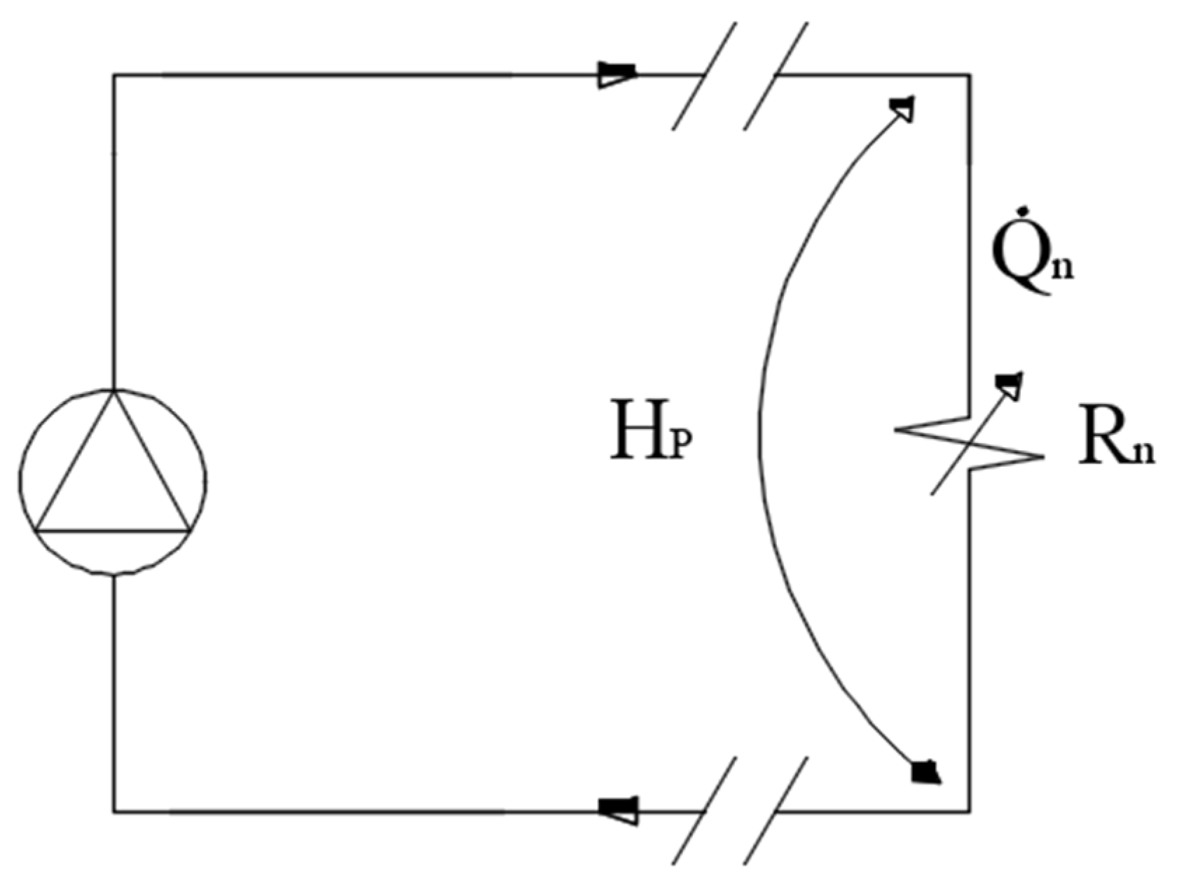
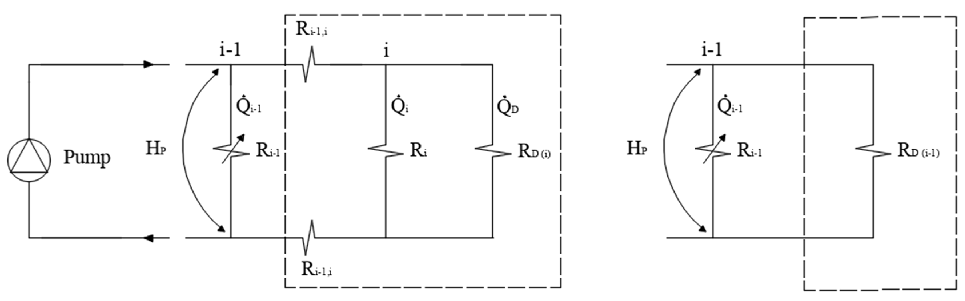
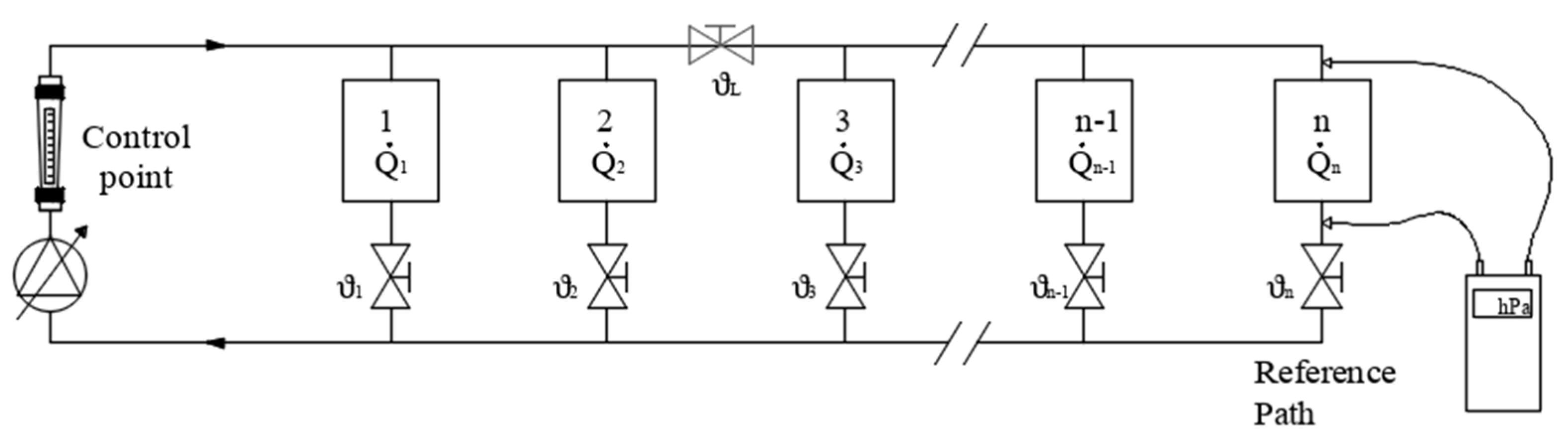
3.1. Progressive Flow Method Theory

The studied method was originally developed for air systems in order to overcome the iterative nature of classical methods, in the form of application of the same methods previously mentioned for water systems TAB: the ratio method and step-wise method.
The assumptions that led to its validation in air systems are considered still valid in water systems; these consist of constant density and a quadratic relationship between velocity and pressure drop under the assumption of a fully turbulent flow regime (ASHRAE [30]).
The lumped-parameters representation of a supply air system (Figure 2) is formally the same as that of a close-loop water system, with the notable difference that in an air system, the return path through the atmosphere has no pressure losses, whereas the hydronic piping is affected by pressure drops due to friction in the return path. In the transposition of the method from air to water, the air diffusers have been replaced by the terminal users’ exchangers, the fan replaced by a pump, and the dampers replaced by balancing valves. The main physical parameter considered in the model is the loss factor R due to friction in pipes and fittings, the overall value of which can be suitably increased by throttling the balancing devices. The relevant quantities considered by the equations are flow rate Q ˙ [m3 s−1], pressure drop P [Pa], and the head pressure provided by the pump H [Pa].
In addition to the shared characteristics, the two systems also have differences in actual installations, the most significant of which for the purposes of this research is the tightness. One of the consequences is that while the performance validation of an air systems requires the measurement of the flow rate exactly at the terminals because of air leakages along the ducts, the tightness in the case of water systems allows cumulative measurements to be carried out; according to mass conservation, the branch flow rate is equal to the sum of the flow rates of terminals belonging to that branch, and the flow rate at the pump is equal to the sum of the branches’ flow rates.
This fact does not lead to any optimization in balancing procedures when using the standard iterative methods or CM, which require flow meters at each terminal. In contrast, in the case of the PFM, the tightness is fully exploited in order to obtain a significant improvement: as described below, flow measurements can be carried out at a single point (e.g., at the pump) while measurements at the terminals can be replaced with an easier to do acquisition of the pressure difference across the user or, in some cases, with the measurement of temperature difference (S. C. Sugarman 2014) [31].
In any case, the analysis of the theory behind the method does not distinguish the way in which the flow rate is measured. This distinction is addressed in terms of further optimization, when the application procedure of the method is presented.
The theorical framework of the method was developed considering the lumped-parameters model previously shown in the lower part of Figure 2.
The relationship between the pressure drop ∆P [Pa] on a straight section (major/distributed losses) as well as across fittings (minor/local losses) and the volume flow rate Q ˙ [m3 s−1] is assumed to be
P = R · Q ˙ 2
where R [Pa·s2·m−6] is the loss factor, whose overall value for major losses depends on piping geometry, (length and diameter), fluid properties (density), and friction factor f; for minor losses, R depends on the geometry of fittings and components (i.e., curves, tees, exchangers, balancing valves) and can be expressed by means of density, average fluid velocity, and the geometry- and size-dependent loss coefficient k [30].
In the following, the value of f is considered constant within the typical operating range characterized by a fully turbulent flow, so R is assumed to be non-dependent on the flow rate value and dependent only on the actual setting of the balancing devices.
In case of series and/or parallel arrangement of the components, the relationship (1) can be used appropriately to describe any portion of a system by means of an equivalent loss factor.
-
For the series configuration of two components or paths whose loss factors are indicated respectively as Ra and Rb, the following applies:
R S a , b = R a + R b
-
For the parallel configuration, the following applies:
R P ( a , b ) = 1 1 R a + 1 R b + 2 R a · R b
These relationships can be combined to create a model through which balancing methods can be tested and subsequently verified experimentally.
From the perspective of how to identify the final balanced configuration, a method is proven to be non-iterative when the parameters whose values are to be assigned are introduced progressively one by one so that the value of every new considered parameter depends only on (i) the design values and (ii) values already determined as a result of a previous calculation or measurement. In this way, at each step, an unknown quantity can be calculated immediately by means of an explicit relation or, in the case of application to a practical procedure, by means of a single calibration/measurement operation that does not involve any further modification of what has been set previously.
On a procedural level, this means that the system is operated in such a way that in each current operation, a measured flow rate depends on the position of a single valve, so that its correct position can be easily found by adjusting it until the desired flow rate value is reached.
This requires a logic of bottom-to-top engagement of the circuits and the observance at each step of a system flow condition that maintains unchanged the flow rates and settings adjusted in previous steps. So, in order to guarantee the progressive involvement of the parameters to be regulated and avoid any back effect of the new balancing actions, the following conditions are necessary:
-
the procedure starts from the farthest terminal by giving a clear criterion to set the adjustment of its valve position;
-
the operator moves backwards and just one terminal at a time is involved;
-
a specific control is introduced in order to keep downward (already adjusted) quantities (flow rates and valve positions) unchanged.
The introduction of such a control is shared by the CM and PFM, with the difference that the PFM provides that the mentioned control can also take place in real time by means of a control loop acting on the portion of the system upstream of the point currently being balanced, in order to keep the downstream flow conditions automatically unchanged.
Returning to the consideration of the representation of a generic branch (Figure 2), each terminal path (i.e., a radiator, a fancoil unit, or an air-handling unit’s coil) is represented as a parallel ith shunt from the main path, whose R i value can vary from a minimum value (at valve fully open) to an infinite value according to the throttle position of the balancing valve. As it is shown in Figure 3, and referring to the split i-point, three sections can be identified: the upstream part of the system on the left, the i-terminal path, and the downstream D part on the right.
The upstream part of the system can be conceptually replaced by an equivalent pump providing the required flow rate Q ˙ D + Q ˙ i at the given head pressure ( H P ).
The downstream part can also be represented by a single equivalent circuit in parallel with the ith path, characterized by the loss factor R D and supplied at the same pressure ( H P ); at the very start of the procedure, the ith terminal itself is the farthest and so, the downward loss factor R D value is assumed to be infinite.
The ith parallel path is characterized by the loss factor R i , which is univocally related to the valve position and whose value can be analytically determined by knowing both pressure and flow rate:
R i = H P Q ˙ 2 i
When the ith terminal is not the farthest, H P depends on downstream conditions:
H P = R D · Q ˙ D 2
where Q ˙ D is the sum of all the flow rates at the terminals in the downstream portion.
So,
R i = R D Q ˙ D 2 Q ˙ i 2
The procedure has been developed in such a way that R i has to be defined only when the downstream resistance values are already defined, so that R D is known and R i can easily be calculated.
The analytical step of calculating the value of R i corresponds, in the practical procedure, to the adjustment of the balancing device which allows the flow rate value Q ˙ i to be reached while the simultaneous maintenance of the flow rate value Q ˙ D is kept.
According to the previous description, the procedure to be followed when R D is known is clear; however, the first step still needs to be defined. At the very start of the procedure, and referring to the last terminal ( i = n ) , the situation is quite different (Figure 4), and Equation (6) can be written as
R n = H P Q ˙ n 2
H P cannot be calculated using (5) because there is no downstream section already calculated, and for any value of H P there is a correspondent value of R n giving the designed Q ˙ n flow rate value; so, one additional criterion has to be considered. This criterion can be found via applying the minimum energy requirement; at the design flow rate, the loss factor has to be as low as possible, so the additional information needed is given by consideration of the maximum opening of the valve as the first step of the PFM procedure.
Back to the general case in procedure, notice that the calculation of R D and H P must be updated at each step by simply by adding the new branch in parallel to the pre-existing downstream equivalent branch as well as the additional line resistance R i 1 , i (Figure 5).
Referring for generality to the (i − 1)th node, as shown in Figure 5 and according to (2) and (3), the following applies:
R D ( i 1 ) = 2 R i 1 , i + 1 1 R D ( i ) + 1 R i + 2 R D ( i ) · R i
Then, applying Equation (6) with updated values, it is possible to calculate the balancing value as
R i 1 = R D ( i 1 ) Q ˙ D 2 Q ˙ i 2
Every time the operator moves to the next branch, the setting of only one new valve position is involved. The action required is the adjusting of the (i − 1)th valve in order to obtain the desired flow rate value Q ˙ i 1 , and the measurement-driven adjustment allows detection of its final value without any iteration. In the meantime, it is necessary to increase the upstream flow rate to flush the new opening path, keeping unchanged all flow rates on the downstream side as well as the pressure at the ith shunt nodes.
If this is the case, it makes no difference whether the Q ˙ i 1 value is measured directly at the terminal or deduced in terms of the increased flow rate provided by the pump.
While the CM involves modulating the position of the partner valve to keep unchanged the flow rate measured at the CBV installed on the index (reference) path, the PFM allows the invariance of the downstream flow rates to be granted by means of simply keeping constant the pressure across the terminal itself, without introducing additional CBV pressure drops. In addition, control of the reference flushing condition can be obtained by alternative ways other than adjusting the branch (partner) valve only, e.g., by varying the pump speed, by opening or closing other upstream branches, or by a combination of all these actions.
If the procedure starts with all the terminals belonging to a specific branch in a closed position, the branch flow rate grows step by step, where each step counts the nominal flow rate of the newly activated terminal, according to the denomination of “progressive flow method”.
As already pointed out in Section 2.2.1, the procedure described in this way allows any branch to be balanced, provided that the farthest terminal is also the disadvantaged one. If this is not the case, the compensated method proposes a subroutine involving measurements and the re-balancing of all terminals.
Considering the most common hydronic system architectures, there are situations in which the position of the disadvantaged terminal is not decisive and an adapted version of the procedure can still be applied without the need to retroactive sub-routines; manifold-based systems and reverse return systems belong to this category. Appendix B examines these systems and shows how the procedure can be adapted and applied.
All other cases (i.e., direct return water systems) point to a situation that is rather common in air systems, which the PFM has had to deal with since its very first formulation.
This critical issue has been addressed from a conceptual perspective and the conclusion is that, given the presence of valves in the proper positions, the general balancing theory can be applied in a more extensive manner and an extended procedure can be applied without the enforcement of any retroactive subroutines.

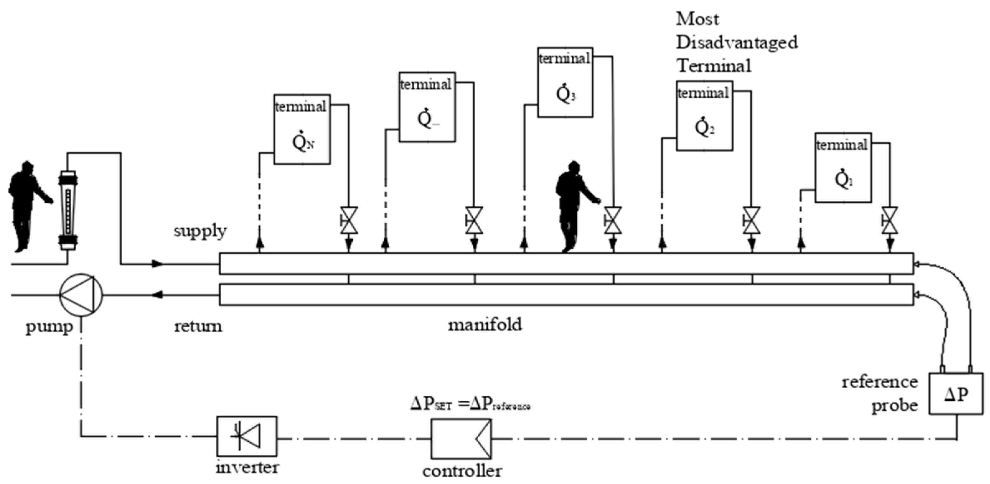
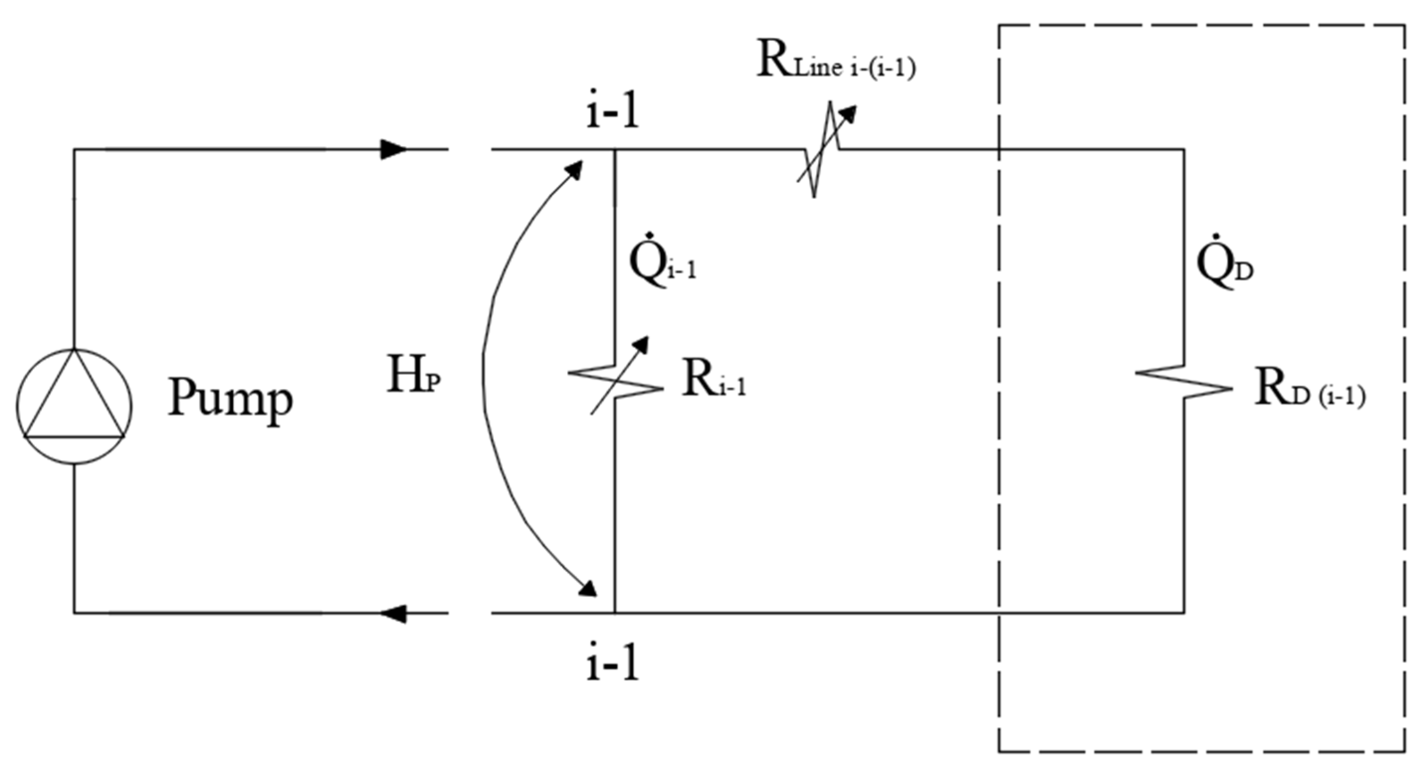
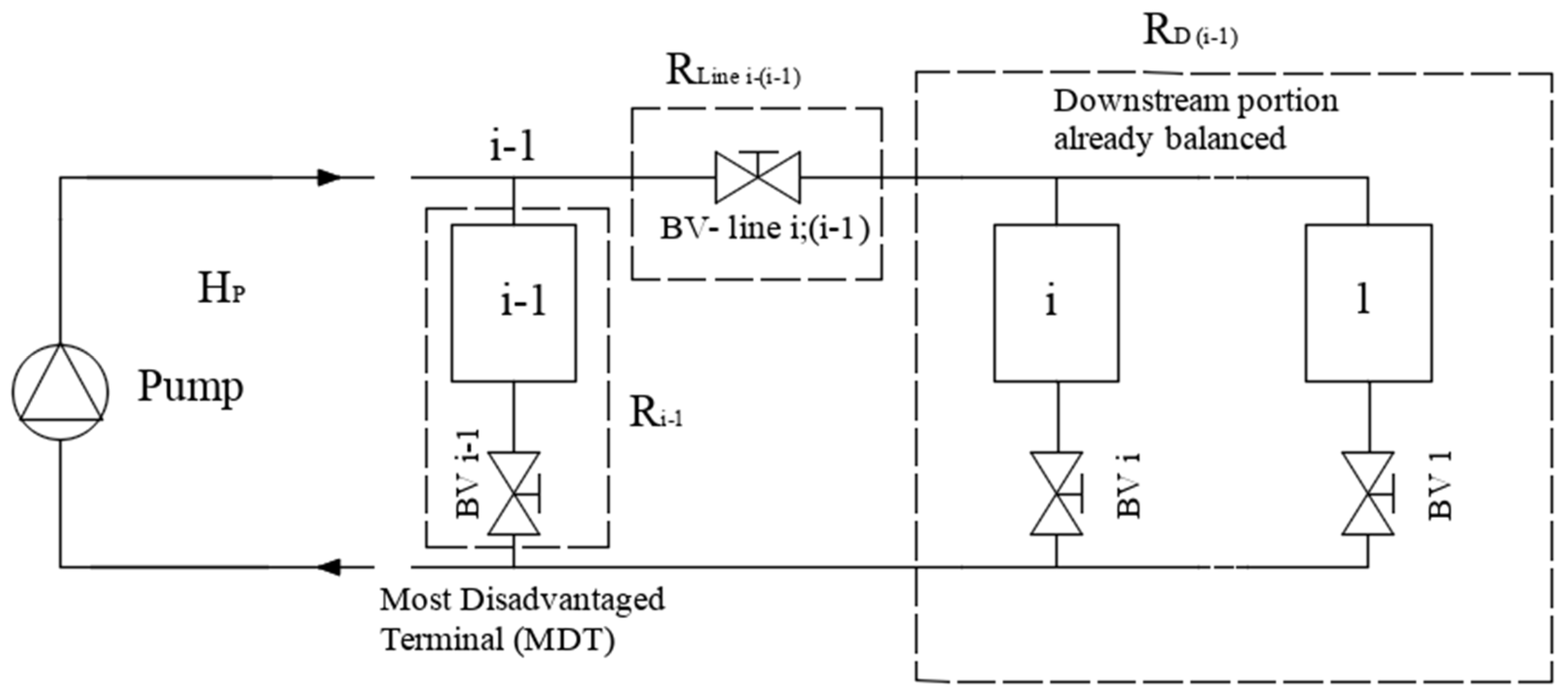
3.2. Management of Cases Where the Farthest Terminal Is Not the Most Disadvantaged

The configuration can be examined with reference to Figure 6, where two different paths are represented branching off from (i − 1) points: the first corresponds to the (i − 1)th branch which has to be activated; the second, on the right in Figure 6, consists of the downstream part of the system, represented by the equivalent loss factor ( R D ( i 1 ) ), which is assumed to have already been balanced.
According to the general theory of balancing in case of ramification, a choking action in the favored path is required, and this implies the availability of a balancing device on it. In cases where the favored circuit is downstream, the requirement can be satisfied by the presence of an adjustable line loss ( R L i n e   i ( i 1 ) ) whose throttling action affects all downstream terminals equally and does not affect their pre-existing mutual balancing.
Analytically, in cases where the (i − 1)th path is disadvantaged, the proper value of the additional line resistance R L i n e   i ( i 1 ) depends on the new path loss R ( i 1 ) 100 (the resistance of the (i − 1)th path with the valve BVi−1 in 100% open condition), on the equivalent resistance of the downstream part already balanced R D ( i 1 ) , and on the flow rate values Q i 1 and Q D :
H P = R ( i 1 ) 100 × Q i 1 2 = R L i n e   i ( i 1 ) + R D ( i 1 ) × Q D 2
R L i n e   i ( i 1 ) = R ( i 1 ) 100 Q i 1 Q D i 2 R D ( i 1 )
In terms of system equipment, the requirements are shown in Figure 7.
In practice, while the automatic control loop (or an assistant operator) acts on the system (i.e., on the pump), maintaining unchanged the downstream quantities, the operator starts to open the valve BVi−1 and the (i − 1)th terminal begins to be flushed, causing a decrease in the downstream flow rate, which is assumed to be immediately compensated by the upstream control. When the terminal valve is fully open, if the flow rate Q i 1 still does not reach the nominal value, this means that the (i − 1)th terminal is actually the MD. Then, the operator moves to act on the line valve BVliIe i;(i−1) and begins to close it, and the flow deviation combined with the loop compensation increases Q i 1 up to the desired value.
As mentioned before, the flow rate measurement required for this operation can be performed directly on the (i − 1)th terminal if a local flow meter is available; in case it is not, it is possible to measure the total flow rate coming from the pump, whose target value corresponds to the value of the previous downstream flow rate (unchanged) increased by the nominal value of the newly added terminal.
In any case, the line resistance can be introduced by installing a simple device capable of introducing a modulable pressure drop without any measuring features. Since it is assumed that the pipeline designer knows which terminal will be disadvantaged with respect to the part of the system that remains downstream, the design can provide for the presence of appropriate line balancing valves, allowing the complete PFM procedure to be carried out.

3.3. Optimization of the Number of Flow Meters and Measurements

A second significant implementation can be achieved by reducing the number of flow meters, resulting in lower installation costs and easier application of the method to existing systems in need of balancing; moreover, the centralisation of measurements saves the time needed to move instruments during the TAB procedure. As previously mentioned, due to the tightness of water systems, flow measurement at the terminals can be avoided and replaced by centralized flow rate measurement combined with simpler reference pressure measurements on only one terminal per branch, whose position depends on the branch configuration type, as follows:
-
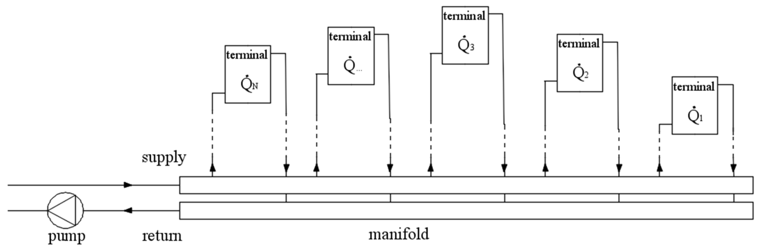
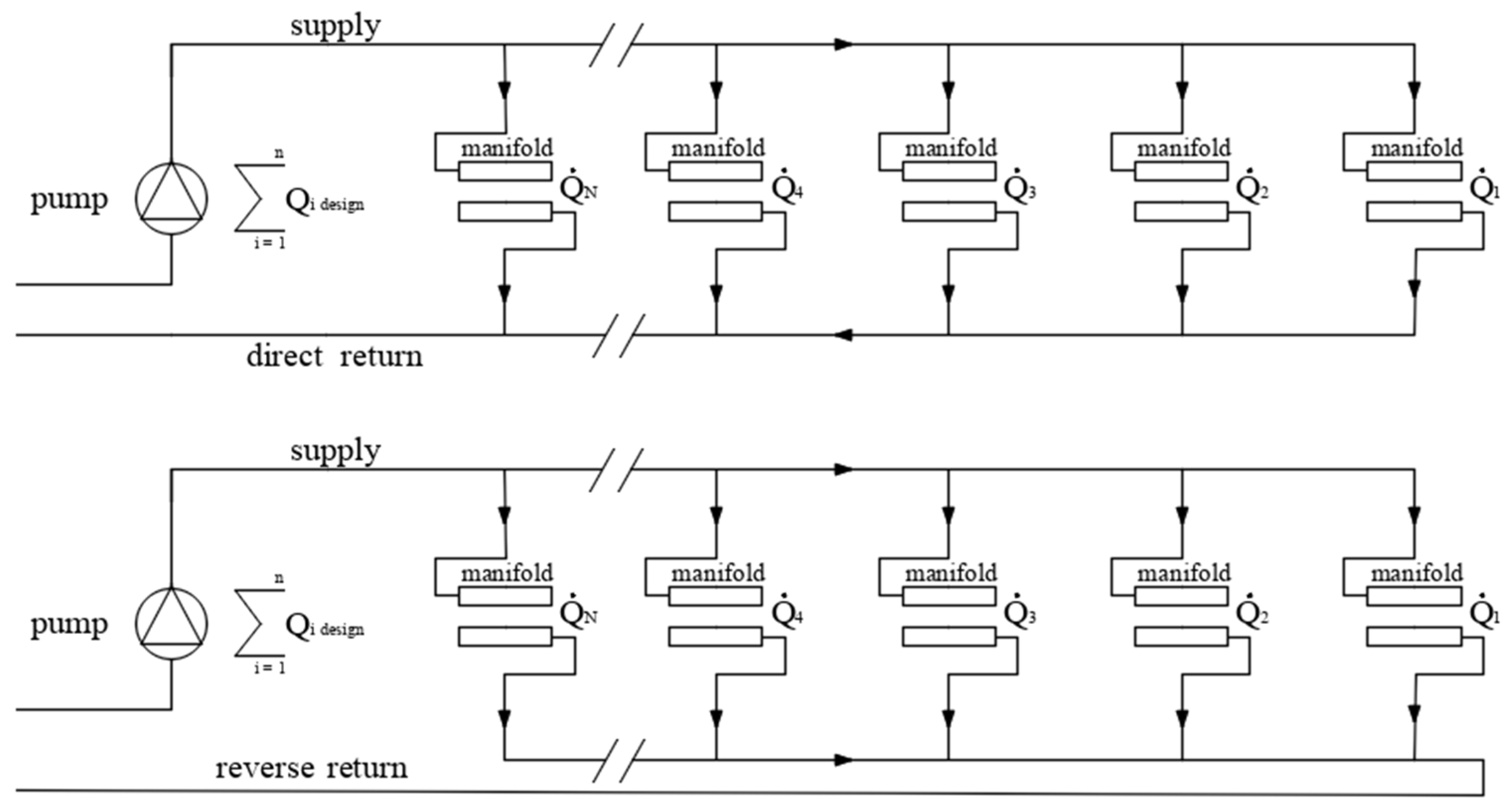
on the farthest terminal in direct return configurations (provided that the line valves are installed where needed);
-
on the most disadvantaged terminal in reverse return configurations (see Appendix B);
-
on the manifold itself in manifold-based configurations (see Appendix B).
If balancing starts with all the terminals in closed position, their progressive activation results in step-by-step increasing of the total flow rate, whose magnitude is given by the volume of water flowing into the newly activated terminal. With the right procedure, this allows measurements to be centralized without any problems of distance between the flow meter and the device being adjusted.
The choice of the control point and of the flow rate measuring system must comply with the following specifications:
(1)
Consistency: the variation in flow rate resulting from the activation of any terminal can be detected at the considered measuring point;
(2)
Resolution: the range and the resolution of the instrument installed at the control point are suitable for the acquisition of the total flow rate supplied to the portion of the system under balancing and for the correct detection of each increasing step, respectively.
If both conditions (1) and (2) are met, it will be possible to proceed with balancing via properly instrumenting a smaller number of flow-meters (or even only one, at the pump).
As far as consistency is concerned, it is important to emphasize that this condition must only be met during the balancing phase and not during normal operation. One way of achieving this may be, for example, to shut off branches other than those currently under balancing. As for compliance with the condition of resolution, with an increasing number of terminals, the flow meter is required to provide a wider measuring range and at the same time a finer resolution. This can be fulfilled by installing two or more instruments with different ranges and resolution placed in parallel and activated as required.

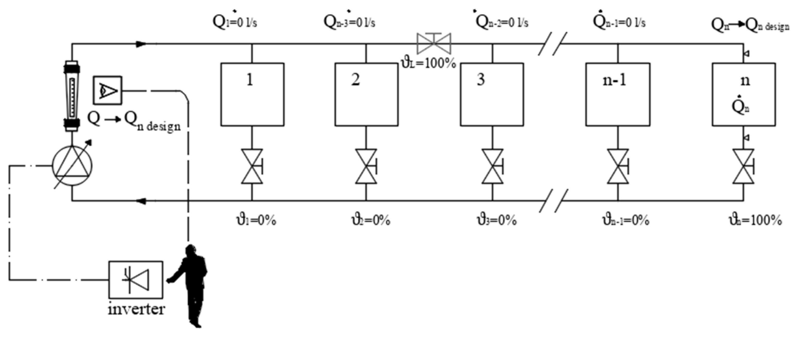
3.4. PFM Balancing Procedure

On the basis of the theoretical elements outlined above, a procedure was developed and is here proposed as a PFM procedure.
Figure 8 shows the case of a system in direct return configuration, with a single branch and n terminals, each with a balancing device. If the designer has determined that the most disadvantaged terminal is not the farthest (e.g., the MD terminal is Terminal 2 as shown in Figure 8), a line valve may be provided (shown in grey), as discussed above. The balancing procedure involves the monitoring of the pressure across the last terminal on the right (the farthest) and the flow rate measurements at the control point placed after the pump, represented by a rotameter. The pump is driven at variable speed and is suitable for inclusion in an automatic control loop when required.
The procedure has been designed as follows:
Preliminary Setup. All the balancing valves shall be closed with only the exception of the one serving the farthest, which has to be fully open. In case of presence of line valves, they must be fully opened as well. For stability of pump operating at low flow rates, it may be appropriate to provide a modulating bypass across the circulator.
First step. (Figure 9). Measuring the flow rate at the control point (represented by the ‘watching eye’ icon), the pump velocity is varied until the flow rate measured by the rotameter reaches the design value of the n-terminal Q ˙ n .
Second step. (Figure 10). An automatic control loop is implemented to keep unchanged the flow rate at the n-terminal acting on the pump velocity. In order to do that, a probe is connected to the pressure taps across the terminal and the actual value is taken as reference. Then, a controller is electrically connected to the probe and to the inverter. The set on the loop controller is Δ P s e t = Δ P r e f e r e n c e .
Third step (balancing). The operator acts on terminal balancing devices or on line valves. Each user is balanced, starting from (n − 1) and moving backwards (Figure 10) to the first terminal of the branch. At each new path considered, the gradual opening of the valve causes a reduction in the reference pressure, which is immediately compensated by the loop control. In most cases, the terminal that has just been opened, compared with that previously activated, is not disadvantaged; the valve is throttled to a opening position lower than 100% and the correct balancing position is detected. When a disadvantaged terminal (e.g., Terminal 2 in Figure 10) is encountered, the total opening of the terminal is not sufficient to guarantee the desired flow rate through the user, so the operator moves to act on the line valve according to the theory. Then, the procedure continues as planned to the next terminal.
If the system is multi-branch, each branch is assumed to be equipped with a balancing device. After balancing the terminals belonging to each branch, the next step is to achieve balance between different branches, following the same strategy as before: starting with all branches closed, first open the reference branch completely, bring it to nominal flow rate conditions acting on upstream components (e.g., on the pump), set the reference pressure loop control, and progressively open all the other branches in sequence, as described previously.
Again, the application of the PFM in direct return systems requires the presence of line valves downstream of the disadvantaged branch if this is not also the farthest.
Fourth step (adjustment). According to the procedure, the pump speed is continuously adjusted through the reference pressure control following the previous steps, so that each terminal is brought to and maintained at its nominal flow rate. The adjustment phase requires only the following actions to be performed:
-
take note of the final speed reached with the setting of the last terminal/branch;
-
remove the reference pressure control loop;
-
set the registered speed as the operating speed of the pump;
-
check that the power consumption and the working point are consistent with the pump manufacturer’s specifications.
At the end of the procedure, it can be verified that at least one path is clear (with no valves even partially closed); that path is the most disadvantaged one. The pump provides the pressure needed for that path and the minimum energy/pressure requirement is fulfilled.
In cases of manifold-based systems, the procedure is the same with the only difference that the reference pressure probe can be installed on the manifold itself; such a case is examined and illustrated in Appendix C.
Cases with systems composed of a main manifold connected to a number of risers each supplying local manifolds with several terminals are also very frequent. This type of case is also described in detail in Appendix C.
Finally, a case where several direct return distribution sub-systems branch off from a single manifold can be considered as a more general case. For this reason, this model was used as a case study for the experimental validation of the method.

3.5. Experimental Validation

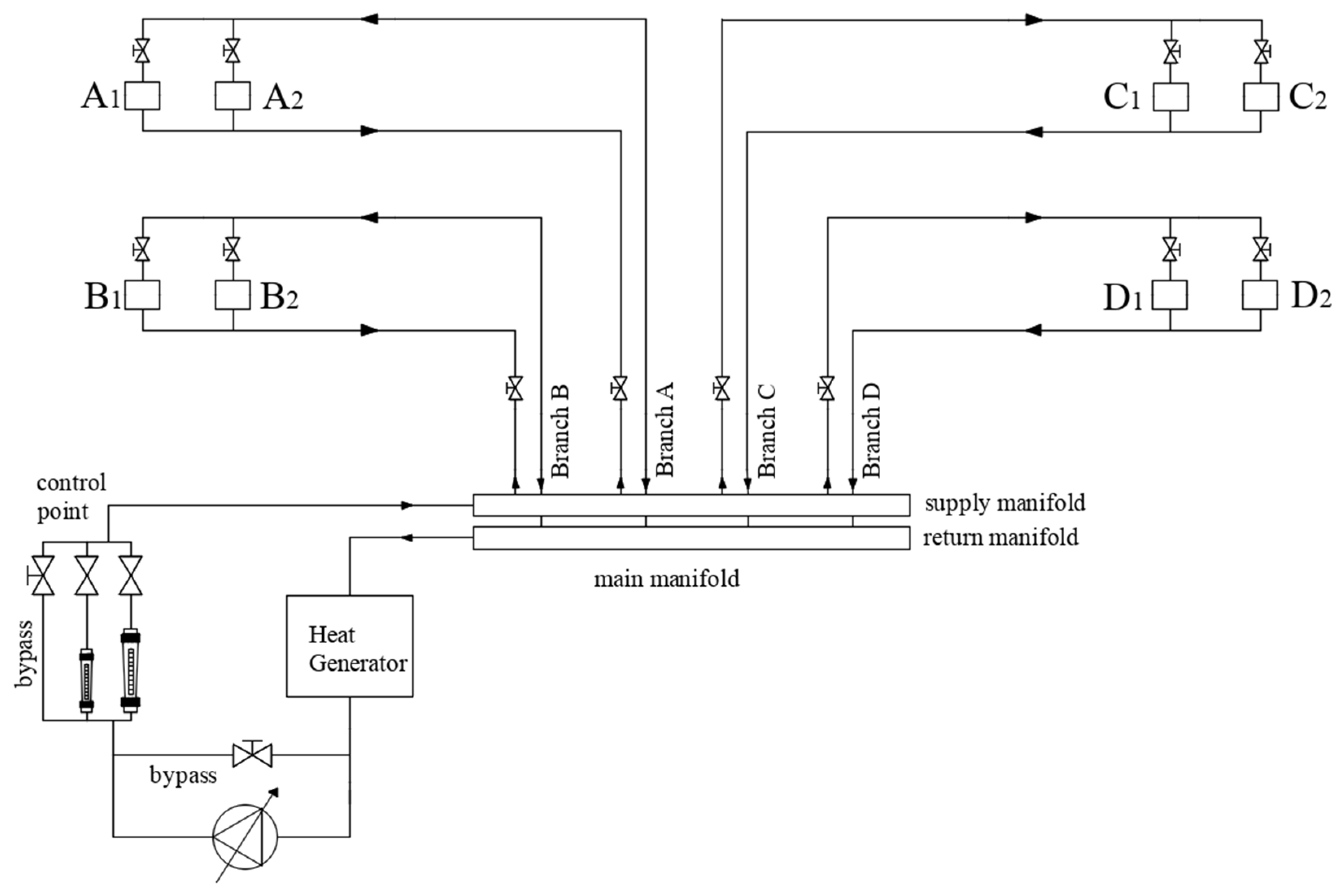
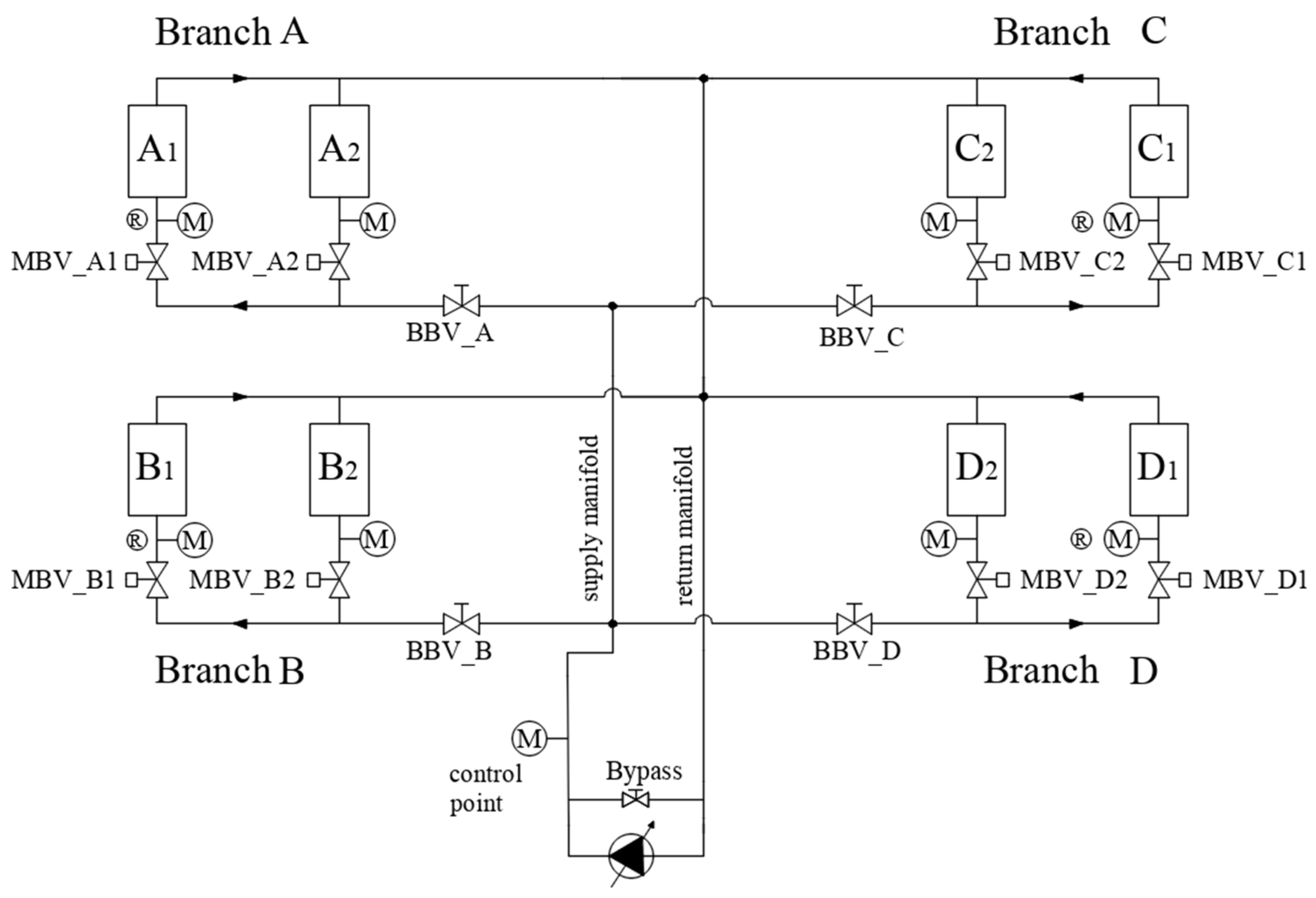
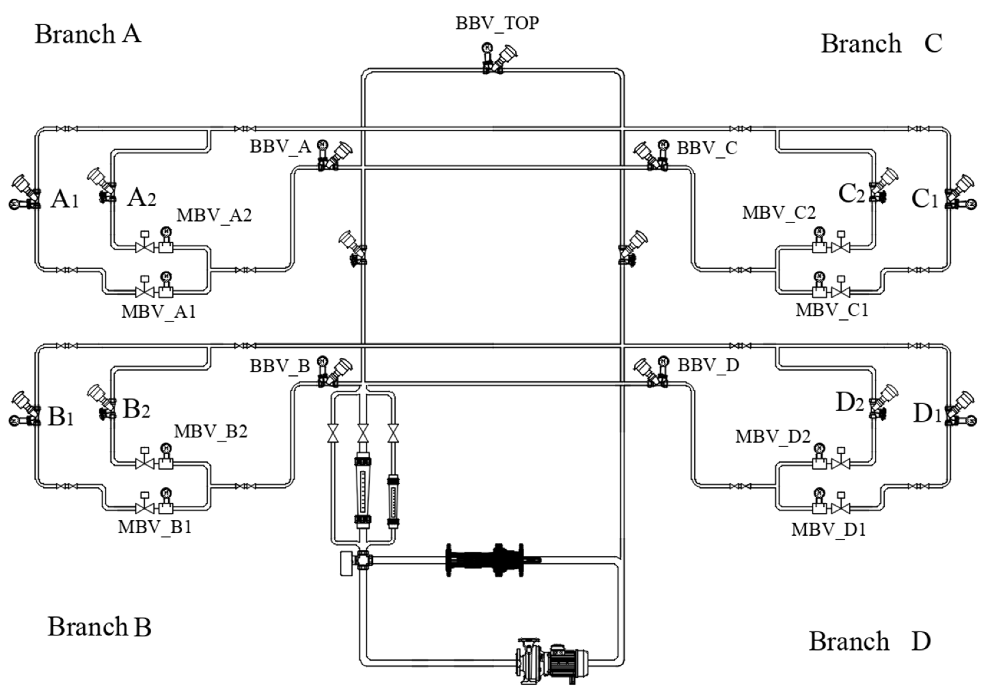
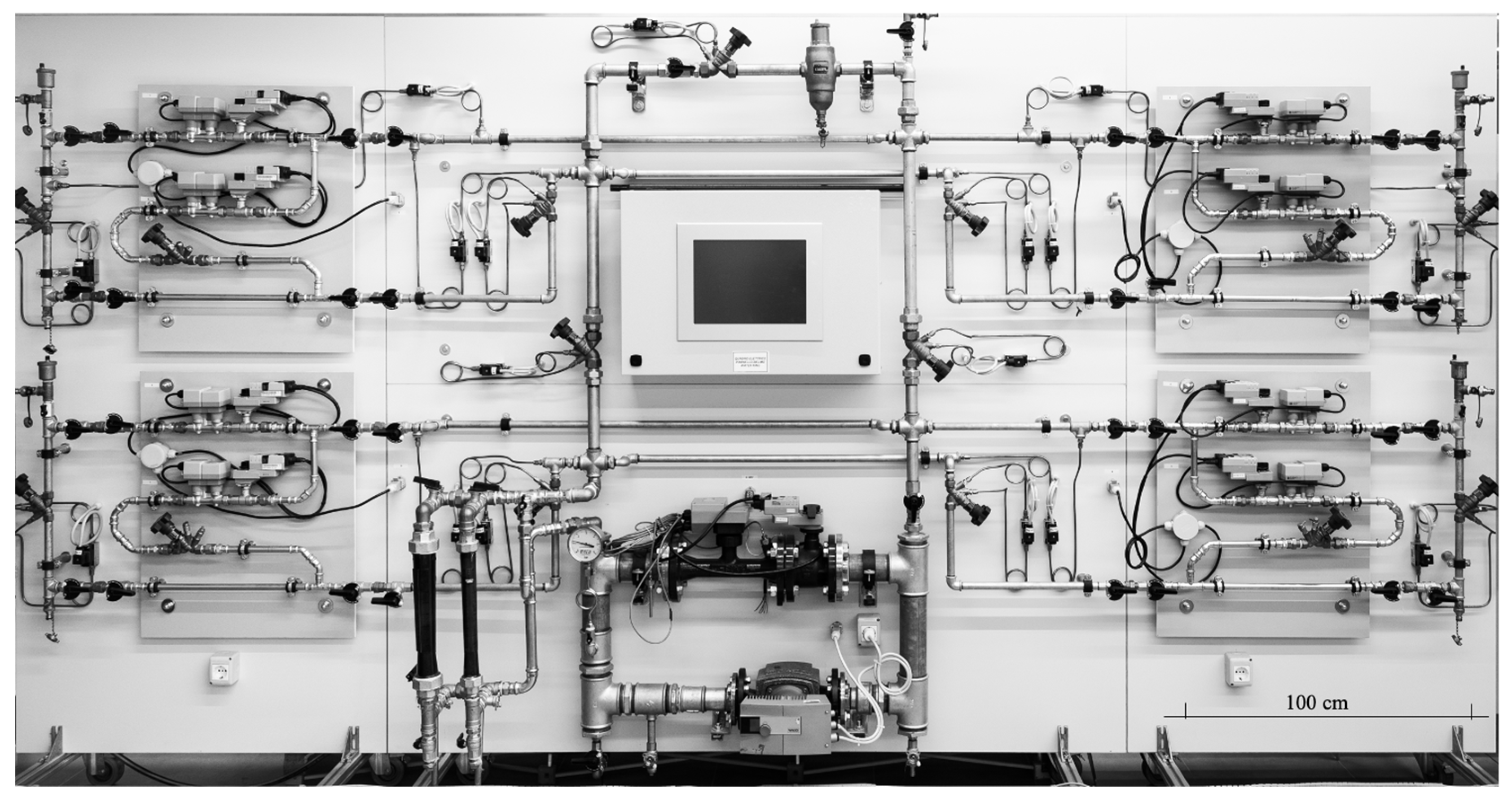
3.5.1. Test Rig Description

In order to validate the proposed procedure, it was decided to compare the PFM with the standard ratio method (RM), on a real water system of enough complexity to highlight the specificities of the two procedures. The implemented circuit consisted of a significant number of terminals (eight in total) distributed two-by-two over four branches derived from a main collector, as shown in Figure 11.
The adopted configuration made it possible to verify the balancing procedures applied firstly at the terminal level (in pairs) and then at the branch level, combining the manifold-based architecture and four double-user sub-systems. Flow measurement at terminals was conducted using ultrasonic probes embedded in electronically controlled Belimo EP015R flow valves, differential pressure measurement across the users was acquired via Thermokon mod. DPL1V differential pressure probes, while central flow measurement at the pump was carried out using Frank M350 rotameters. A detailed description of the circuit, the type of control and the measuring instruments used can be found in Appendix D. Figure 12 shows a picture of the realized test rig and Table 1 shows the main information about the measurement equipment used.

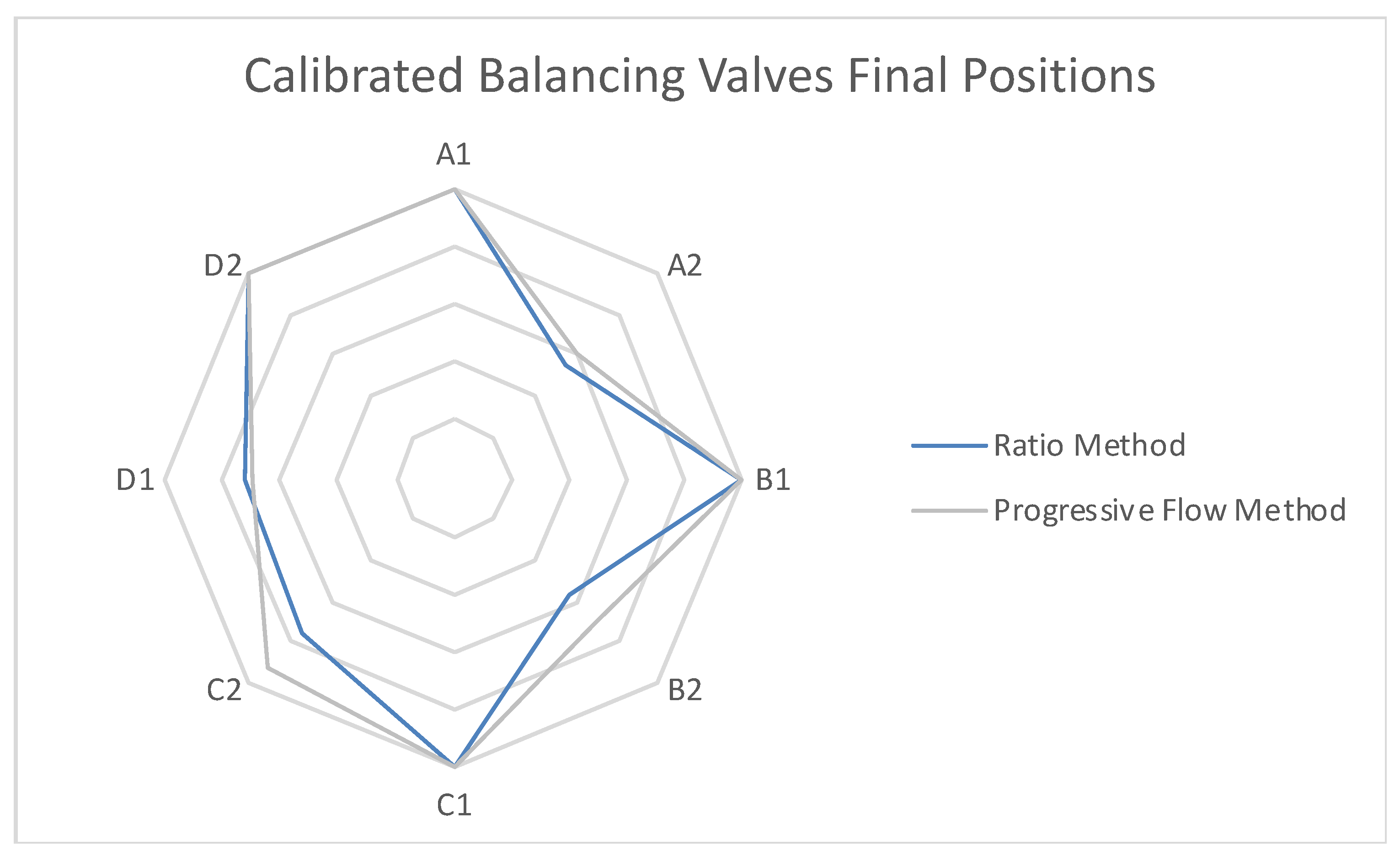
3.5.2. Comparison between Ratio Method and PFM

First, a set of target flow rates was defined as well as a balancing tolerance value of ±10% for individual flow rates, according to the standard requirement (ASHRAE and NEBB [28,29,32]) and international commissioning associations such as the Building Services Research and Information Association (BSRIA) [33].
Nominal pressure drop values of the simulated terminals were defined with reference to typical hydronic terminals, and the determined values were obtained by adjusting the calibrated balancing valves positioned for that purpose.
This configuration applies to a real case of seven fan coil units (from A2 to D2) characterized by head losses of about 5 kPa with quite different nominal values of flow rate, and one different type (A1) representing a manifold serving an underfloor heating/cooling system whose loss is estimated at 30 kPa. The established flow rates, referring to a working Δ T = 5   ° C , led to heating capacities values consistent with the defined types.
Table 2 shows the system design configuration and lists the assumed thermal powers, design flow rates, pressure losses, and handwheel position of the drop simulation valve for each thermal unit (TU).
As the two methods refer to different flow meter readings, the comparison of the results required an initial consistency check of the measuring instruments. The full test carried out is described in Appendix E. The main result was that in the range of flow values to be considered for comparison, rotameters overestimated the measurement by an average of 4.9% compared with ultrasonic probes (Appendix E Table A1).
After the adjustment step, the PFM (higher measuring rotameter-referred) is expected to lead to a pump speed that is lower than the velocity obtained after the final adjustment step required by the ratio method procedure (lower measuring MBV-referred). According to the consistency check, the expected difference for pump velocity was about 5%.
However, although at different final speeds, both methods were expected to reach the same proportion of flow rate values according to the design data; so, the most significant validation resulted from the comparison of final valve positions.
After conducting the preliminary set-up activities, the two methods were applied in succession. The step-by-step execution of the two procedures is reported in Appendix F.
At the end of both procedures, the flow values and the positions of all balancing devices as well as the final speed of the pump were registered. It was also verified that both methods led to an effective minimum energy/pressure configuration, with at least one clear path.
Finally, for each method applied, the number of balancing actions Nbal required as well as the number of measurements Nmeas (including the repositioning of the probe instruments) was determined.

4. Results

The results in terms of final flow rate show how the RM led to a balanced situation within tolerances: the terminal with the greatest deviation was terminal C1, which had a flow rate difference of 8.8% from the nominal value. As far as the progressive flow method is concerned, its operation did not involve the measurement of flow rate at individual terminals other than in terms of the increase in the overall flow rate at the time of its activation. In any case, the method proceeded to sequentially activate the terminals only when the updated total flow rate was at the desired value, so the value at the end of the procedure could be precisely adjusted to the nominal value (2600 l/h), within the accuracy limits of the rotameter. After considering this, the equivalence of the two different procedures was assessed by comparing, in addition to the total flow rate just discussed, (i) the final positions of the balancing devices and (ii) the final pump speed. Useful values for comparison referring to both methods are presented in Table 3.
Regarding the final valve configurations and referring to the values reported in Table 3, a radar graph (Figure 13) has been provided to compare the positions reached after the application of each procedure.
The chart highlights some local differences; it may be noticed that the B2 and C2 terminals differed significantly (respectively, 56% to 70% for B2 and 75% vs. 92% for C2).
Application of the PFM did not require direct measurements at the B2 and C2 terminals and so, direct comparison in terms of flow rate values was not possible.

5. Discussion

Regarding the terminal valve positions, the fact that B2 and C2 showed positions that differed by 14% and 17%, respectively, at the ends of the two procedures deserves further investigation: the assessment that needs to be made is firstly whether the difference in flow rate is expected to be greater or less than the difference in valve stroke. Since the valves used in the balancing test rig were control valves, the factors that must be considered for this analysis derive from the theory describing the flow rate/position relationship for this type of valve. These factors are represented by (i) the inherent characteristics of the valves used, (ii) the degree of openness of the valves in which the behavior is to be analyzed, and (iii) the value of the Authority parameter assumed by the valves with respect to the controlled circuit. These valves are designed to maintain equipercentage behavior in the upper half of the opening and the authority calculation gives a value for both in the range of 0.2–0.3. In accordance with ASHRAE [30] and as shown in Figure 14; considering an Authority value within the range [0.2–0.3] (or, in percentage, [20–30%]), the flow rate variations related to the difference in the opening respectively between 92% and 75% and between 70% and 54%, were expected to be lower than 10%, as highlighted by the red and green reference quotas.
As for the speed rotation of the pump and referring to the previously expressed considerations, the difference must be consistent with the difference in measurements obtained by the instruments taken as the reference instruments for each method; the value obtained by applying the PFM method based on rotameters led to a rotation speed of (80 − 85)/80 × 100= −6.25% lower than that obtained with the terminal ultrasonic probe-based ratio method, in good agreement with the 4.9% difference verified by carrying out preliminary consistency tests between the two measuring instruments (Appendix E, Table A1).
After discussing the PFM from the theoretical point of view and its experimental validation, it is considered useful to investigate its practical advantages.
A first evaluation was made by simply comparing the overall Nmeas and Nbal required by the application on the test rig; the values were compared with the ones obtained through application of the PFM, see Table 4.
The PFM proved to be more efficient, both in terms of the actions required for balancing and in terms of movement of the measurement probes; the advantage would increase with greater numbers of users per local manifold. The proposed method turns out to be entirely non-iterative and performs balancing directly at the nominal flow rate without requiring iterations or a final adjusting step. In addition, with presence of the appropriate line valves, the PFM overcomes the critical limitations shown by the other non-iterative method, i.e., the CM.
Lastly, the listed advantages are characteristic of a method that can be applied regardless of the presence of flow meters on all terminals; pressure taps can more easily be provided across the terminals to be used as a reference control and this can be a key factor in balancing existing buildings that are difficult to work on. The simplifications on which the evolution of the PFM originally developed for air systems has been based have essentially been made possible by the opportunity to adopt methods of adjusting the compensation flow rate by means of real-time control, which replaces the time-consuming adjustment phases of iterative methods.
The assumption, which is always verifiable, of perfect tightness of the hydronic piping has a great influence on the method’s operating mode because it allows all flow rate measurements to be reported to a single measuring station located at the pump. However, the full applicability of the method requires specific attention on the part of the designer and, in particular, the ability to determine at the design stage which positions will require the presence of line-balancing valves.

6. Conclusions

The proposed method was investigated, taking into account that there are many existing and new applications for which balancing is required. Traditional methods present the problems of being iterative and requiring direct or indirect terminal flow measurement systems.
The compensated method, which was proposed in the 1990s to overcome the problem of iterativity, also has some drawbacks such as the need to install calibrated balancing valves with flow measurement features on all terminals, and it does not fully address some situations that can be faced during balancing and that require going back in operations.
The proposed method, referred to as PFM and derived from previous studies on the balancing of air systems, is presented from a theoretical perspective and declined for application with reference to the main architectures of water systems; the method has been optimized by appropriately exploiting the tightness characteristic of hydronic networks, making it possible to propose a procedure that does not involve terminal flow measurements but only P measurements across the farthest terminals, which are used as a reference, and a single centralized flow measurement point.
The flow rate detection equipment, consisting of multiple instruments placed in parallel and activated as required, can be used to apply the procedure to all sections of even complex plants according to a logic of scalability that guarantees adequate resolution and measuring range. The measuring tool can be placed in series with the pump during TAB operations and removed after finishing, to be reused on similar installations.
The procedure was tested experimentally in comparison with a standard method (ratio method). The results were validated and both applied methods led to a result within the accepted tolerance of 10% in terms of flow rate and to a comparable configuration of the balancing device.
Finally, savings were quantified not only in terms of the number of flow meters required, but also the numbers of measuring and balancing operations required, which in the case analyzed were reduced by 48% and 41%, respectively.
The research developed in the field of balancing water systems offers interesting insights. In particular, these include developments in the application of general balancing concepts to the field of flow control in variable flow systems and a possible rethinking of the dynamic control modes currently adopted.

Author Contributions

Conceptualization, F.P.; Methodology, F.P.; Software, F.P.; Validation, F.P.; Formal analysis, L.P.M.C.; Investigation, F.P.; Resources, L.P.M.C. and F.R.; Data curation, F.P.; Writing—original draft, F.P.; Writing—review & editing, F.P., L.P.M.C. and F.R.; Visualization, F.P. and F.R.; Supervision, L.P.M.C. All authors have read and agreed to the published version of the manuscript.

Funding

This research received no external funding.

Institutional Review Board Statement

Not applicable.

Data Availability Statement

The original contributions presented in the study are included in the article, further inquiries can be directed to the corresponding author.

Acknowledgments

The authors acknowledge the technical and operational contribution of Belimo Italia in the person of Luca Pauletti. This research did not receive any specific grant from funding agencies in the public, commercial, or not-for-profit sectors.

Conflicts of Interest

The authors declare no conflict of interest.

Abbreviations

Abbreviations
CWVconstant water volume system
VWVvariable water volume system
TABtesting, adjusting, and balancing procedure
CMcompensated method
PFMprogressive flow method
RMratio (or proportional) method
SMstepwise method
MDmost disadvantaged (referred to a path or a terminal)
CBVcalibrated balancing valve
MBVmotorized balancing valve coupled with ultrasonic flow meter
Nmeasoverall count of measuring operations (including moving probes, setting up control loop)
Nbaloverall count of balancing operations (including adjusting valves and pump speed setting)
Nomenclature
Q ˙ flow rate [m−3·s−1] [l·s−1] [l·h−1]
ΔPpressure drop [Pa] [kPa]
ΔTdifference in temperature [K]
ΔH, HPpump head pressure [Pa] [kPa]
Rloss factor [Pa·s2·m−6]
ffriction factor—dimensionless
kloss coefficient—dimensionless
Nmeasnumber of measurement readings
Nbalnumber of balancing operations
Subscripts
SSeries
Pparallel
Ddownstream
irefers to the ith component, path, value

Appendix A. Proportional Method and Step Wise Method Description

Appendix A.1. Traditional Balancing Methods Procedure

With reference to the NEBB manuals, the procedures indicated for the application of the two traditionally used methods for the balancing of constant flow hydronic systems are given in the following steps.

Appendix A.2. Proportional Method (Also Referred to as Ratio Method)

Applied to a generic water system provided with all the required balancing devices, it consists in a step-by-step procedure composed of the following main actions:
1. Preliminary setup. All the valves are fully opened, and the pump is adjusted so that the total flow rate results to be slightly (normally about 10%) greater than the design value.
2. Testing. At this working condition, each terminal flow rate is measured and the ratio Q ˙ M / Q ˙ N between actual and nominal flow rate is calculated for each terminal; referring to the ratio values, all the terminals belonging to each branch are sorted in ascending order from the most advantaged (or “favoured”) to the most disadvantaged (or “unfavoured”).
3. Balancing. Considering one branch at a time, all the terminals are considered in pairs, starting from the two most disadvantaged and acting on the less disadvantaged’s valve to achieve the same rate ratio of the other, according to the accepted tolerance. This process is iterative, since every action on a valve has the effect to change the flow rate of all the other terminals so that the operator is supposed to move back and forth between the two users, checking every time the actual ratio. When they result to be balanced, the third terminal in the ranking is taken into account and brought to the same ratio of the previously balanced pair (i.e., considering it in a pair with the original MD), thus proceeding to the next and going in this way up to the last one, which is also the one that was originally the most favored. This progressive arrangement leads all terminals to the same ratio value and at this point the branch can be considered balanced.
If there is more than one branch, the users belonging to each one can be balanced between them following the same procedure, then all the branches can be balanced in the same way by acting on the branch-valves and following the same pair procedure. At the end of the balancing step, the whole network is characterized by the same rate ratio within admitted tolerances.
4. Adjusting. The pump velocity is varied, and all the flow rates will increase (or decrease) at the same time until the shared rate ratio reaches the unit value and the total flow rate reaches the nominal value.
The balancing procedure involves iterations because after any action on a valve the flow rates of all other paths change as well. This makes the procedure expensive in operations and time. Furthermore, results and time consumption strongly depend on the system complexity, the required tolerance, and the operator experience.

Appendix A.3. Stepwise Method

It is a step-by-step procedure consisting of the following main actions:
1. Preliminary Setup. All the dampers are fully opened, and the pump is adjusted so that the total flow rate results to be slightly (normally about 10%) greater than the design value (same as RM procedure).
2. As the flow rate at the terminal closest to the pump will typically be the highest, adjust the balancing valve aiming to a flow rate value approximately 10% below the design flow requirements, then move to the following terminal and repeat the same action. As the adjustment proceeds to the end of the system, the remaining terminal flow values will increase.
3. Repeat the adjustment procedure throughout the system until all terminals are within ±10% of the design flow requirements and at least one path valve is wide open.
4. If necessary, adjust the pump velocity to set all terminals at ±10% of the design flow, check once again all the terminals, register final values and eventually mark the position of all the balancing valves.
As in the case of the Ratio Method, the Stepwise method involves iterations (with the related drawbacks); in addition to that it’s not clear from the beginning which path is the most disadvantaged, so it may occur the operator closes a valve belonging to the MD path, disregarding in that way the minimum-energy/pressure requirement.

Appendix B. Analysis of Cases Where the Farthest Terminal Is Not the Most Disadvantaged

The situation where the farthest terminal is not also the most disadvantaged is a critical situation for the application of the CM-compensated method and of the method proposed in this paper, and the conceptual and procedural overcoming of this issue for the most general case has required the in-depth discussion presented in Section 3.2, however, for some configurations, a simplified method can be followed.

Appendix B.1. Manifold-Based and Reverse Return Cases

In case of manifold-based water systems (Figure A1), this issue is easily faced since the presence of the manifold allows the concept of farthest user to be overcome; in fact, if the manifold is properly sized it offers negligible pressure drops and all user branches in parallel are supplied at the same pressure.
Figure A1. typical manifold- based local user system.
Applsci 14 06232 g0a1
In such cases, the procedure can be adapted by starting not from the farthest but directly from the most disadvantaged MD terminal. A suitable solution is also the installation of pressure taps directly on the manifold and using the differential pressure between supply and return manifold as the reference.
If this is not practical, and it is preferred to take one terminal as reference, it is required to identify the MD terminal: the techniques for MD terminal detection are reported in the following.
The reverse return configuration presents quite an analogy with the manifold-based case; the working pressure of each user is invariant because of the connection as the different allocation of line drop losses between supply and return are composed in such a way as to be self-compensating. This makes these two types of circuitry (manifold-based and reverse return), conceptually assimilable each other and can be approached in the same way, simply by identifying the MD terminal and starting from that. The assessment proposed for the detection of the MD path can also be applied to the case of reverse return systems, with some small (and described) adaptation.

Appendix B.2. Determination of the MD Terminal in Manifold-Based or Reverse Return Configurations

Firstly, the disadvantaged terminal can be identified in every configuration by the designer during sizing activity. Whatever the procedure of identification, this terminal will assume the role of “reference” or “index” and will be chosen as the starting terminal as discussed in the paper.
In the absence of the appropriate design documentation, it will still be possible to identify the disadvantaged terminal, provided that at least all design flow rates are known.
The determination of the MD terminal can be experimentally carried out in a manner that depends on the availability of terminal flow sensors or a single sensor at the pump (or common section).
(1)
Having individual flow meters available on each terminal user, it is enough to carry out a preliminary measurement with all valves fully open. The most disadvantaged terminal can be found by calculating the characteristic ratio Q ˙ M e a s u r e d / Q ˙ N o m i n a l for each path and choosing the one with the lowest value as commonly practiced when using the traditional Ratio Method (see Appendix A.2).
(2)
Alternatively, by using a single flow meter at the pump, different sub cases must be considered:
(i)
if the terminals are same model and size and connected by piping have similar length, there is no reason why the Q ˙ M e a s u r e d flow can vary, then the MD terminal is by definition the one with the greatest Q ˙ N o m i n a l flow rate value, and there’s actually no need for measurements; this case also arises when terminals of the same size have so significant pressure losses that the path’s differences are negligible.
(ii)
if the design flow rate values of the users are the same but path lengths are different, the flow rate of each terminal can be measured by running the pump at a constant speed and fully opening/measuring only one path at a time closing the others. The calculation of the ratio Q ˙ M / Q ˙ N allows the terminals to be sorted and the MD to be identified.
(iii)
if both lengths and flow rates of each path/terminal are different, the previous test, to be exhaustive, must be conducted by imposing a constant manifold pressure; this requires a pressure detection across supply and return sections of the manifold. That pressure detection can also be used as pressure reference for control loop in PFM procedure.
The reverse return configuration presents quite an analogy with the already discussed main manifold-based case; the working pressure of each user is invariant because of the connection, and the different allocation of line drop losses between supply and return are composed in such a way as to be self-compensating. This makes this type of circuitry assimilable to the manifold-based circuit and can be approached in the same way, simply by identifying the MD terminal as previously described and starting from that; in the absence of a manifold, the pressure measurement related to the (iii) case can be performed directly across one of the connected terminals.
Frequent is also the hybrid case of a main manifold with the departure of distributed lines (e.g., risers serving radiators or fancoils) or the case of a primary distribution serving zone manifolds in sequence with direct/reverse return as shown in Figure A2.
Figure A2. Combined primary distribution supplying local manifold-based user systems with direct and reverse return configuration.
Applsci 14 06232 g0a2
In these cases, local zone manifolds represent complex users which can be conceptually replaced by equivalent users having the total flow rate and design pressure head of the manifold and whose size of which is not related to the position, but generally depends on the heat loads of each zone; in these situations, it can easily happen that the farthest manifold is not also the MD one.

Appendix C. PFM Procedure for Manifold-Based Systems

Considering more complex systems than the case discussed, the procedure can be further refined, but there is no need to introduce additional conceptual elements.
A case to be examined is the case of a manifold-based system or sub-system (Figure A3).
Figure A3. PFM procedure application in case of manifold-based system or sub-system.
Applsci 14 06232 g0a3
As discussed above, the presence of the low-loss manifold makes the order of activation irrelevant, as conceptually it is as if all paths were driven by the same head pressure value. The procedure only requires an initial step to check which is the disadvantaged terminal; once that terminal with the valve fully opened is brought to its nominal flow rate value (first step of the PFM procedure), the pressure at the manifold will be taken as reference and balancing of other terminals starts (second step). In Figure A3 the position of the measuring points is shown, as well as the reference control loop and the operator’s activity.
As a further example, Figure A4 shows a system composed by a main manifold serving more risers each supplying local manifolds with several terminals.
In this case, it is possible to start by applying the PFM balancing procedure to each zone manifold, then repeat it at branch-level and finally proceed similarly at the main manifold level for the balancing of the risers. The same pressure taps can be used as reference for all balancing levels. In the case of large systems the control point can be located far from the system portion under balancing procedure so the electrical connection required by the reference loop can be an issue, as well as the transferring the information of the value of the measured flow rate from the control point to the operator acting on the valves.
Figure A4. system composed by a main manifold serving more risers each supplying local manifolds.
Applsci 14 06232 g0a4
Figure A4 also shows the adoption a multiple scalar measuring system, with a smaller instrument suitable in term of range/resolution for local (range refers to manifold/resolution refers to single terminal), a medium one (riser/local manifold) and a bigger (total pump discharge/riser).

Appendix D. Test Rig Description

The circuit consists of 8 terminals distributed two by two over 4 branches derived from a main collector, as shown in Figure A5.
Figure A5. configuration of the system to be balanced.
Applsci 14 06232 g0a5
Branches are named A, B, C, D, and terminal are referred to by branches and numbers (A1,A2,B1,B2,C1,C2,D1,D2).
Figure A6 shows the layout and the position of the components. The test rig has been realized on a vertical panel; the supply and return sections of the main manifold are positioned vertically and are connected at the top by a bypass which has been kept closed during the tests. The pressure drops of the simulated terminals are replicated by calibrated valves set to be representative of the selected user types (i.e., radiators, fan coils units, air handling unit coils).
Figure A6. Test rig configuration and components.
Applsci 14 06232 g0a6
The system is equipped with balancing devices on each user; these are motorized balancing valves (MBV) coupled with an ultrasonic flow meter integrated in a device normally used for flow control in variable volume systems (Belimo mod. EP015R); the opening position of each valve is digitally controlled via the bus and its actual position is transmitted back to the operator panel.
Branch balancing valves (BBV) are manual calibrated valves whose position is clearly indicated by the multi-turn graduated handwheel and whose flow measurement feature is only used if/when required by the TAB method being used.
The accurate position detection of all the valve types is useful to compare the balancing configurations achieved by the tested balancing method. The set-up is completed by the adoption of a pump speed control combined with an adjustable bypass for more precise volume modulation.
With regard to the measuring points, the two methods to be compared involve different detections: the Ratio Method requires flow measurements at each terminal, whereas the PFM method only requires instrumenting the reference terminal of each of the four zones (A,B;C;D) with pressure taps and a single flow meter at the pump.
The ultrasonic flow meters at the terminals (MBV) present declared accuracy of 6% of the reading value ranging from 25% to 100% of the measuring range of 0–1200 L/h.
The control point at the pump is instrumented with two rotameters (Both Frank mod. M350, different size, declared accuracy of 8% of measured value for flow rates between 20% and 100% of measuring range according to VDE/DIN 3531), the two instruments are placed in parallel as shown in Figure A7.
Figure A7. Rotameter flow meters, with bypass branch for maintenance operations.
Applsci 14 06232 g0a7
According to general criteria for centralized measuring discussed in Section 3.3 of the paper, the two rotameters have a measuring range, respectively, of 50 ÷ 500 L/h and 300 ÷ 3000 L/h. In this way, managing and running only the appropriate instrument, the flow rate can be measured with the accuracy, range and the resolution required at each step of the PFM procedure. Figure A7 also shows the bypass branch provided for easier maintenance operations.
Finally, the calibrated valves installed to simulate the terminals’ drop losses are provided with pressure taps. The taps were connected to pressure probes (Thermokon mod. DPL1V, declared accuracy 1%, resolution 0.2 kPa) to be used as reference when required by PFM procedure.
All active probes and electrically controlled actuators are managed by a bus control system capable of PID logics and data acquisition/elaboration. A large display shows actual operating parameters and values (i.e., the current flow rate values, pressure drops, motorized valves position, total pump flow rate, electric consumption, pump speed).
The construction drawing is shown in Figure A8.
Figure A8. Test rig construction drawing.
Applsci 14 06232 g0a8
The pipework and pump are sized for a total flow rate of 0.833 L/s (3000 L/h), the pipes are sized according to a speed range of 1 ÷ 1.5 m/s, maximum terminals’ pressure drop is 30 kPa (consistent to the typical drop values of fan coil units, AHU coils or an underfloor heating/cooling system). The variable speed pump is sized to provide a head pressure of 80 kPa, which also considers the presence of the auxiliary components and fittings such as non-return valves, filters and measuring devices.

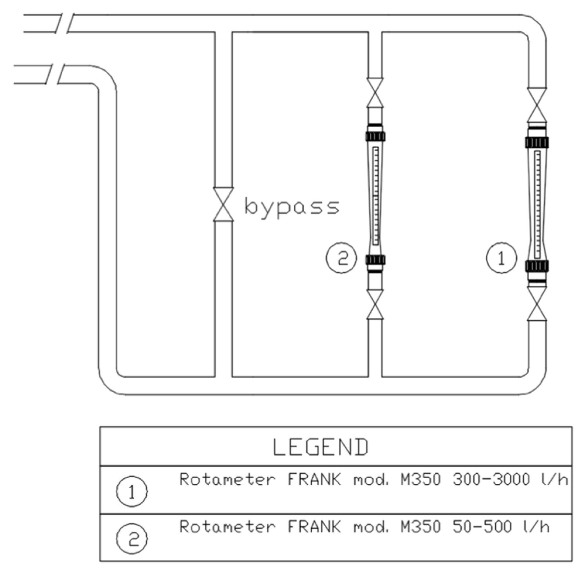
Appendix E. Consistency Check between Rotameters and Ultrasonic Probes

The test was carried out between the measurement made with the ultrasonic probes MBV at the terminals and the measurement made with the rotameters at the pump. The test was conducted by opening only one terminal at a time at three levels of flow rate (33%, 66%, 100% of MBV full range 1200 L/h), thus measuring the same flow rate with both instruments and calculating the difference in terms of percentage and ratio (K), Table A1 shows the results of the measurements described.
Table A1. comparison of measured values at 100%, 66%, 33% of 1200 L/h (full scale of the MBV ultrasonic probes).
BranchTerminal UnitFlow Rate 33%
(400 L/h)
ΔFlow Rate 66%
(800 L/h)
ΔFlow Rate 100%
(1200 L/h)
Δ
RotameterMBV[%]KRotameterMBV[%}KRotameterMBV[%]K
AA14003736.80.9380071510.60.891200105012.50.88
A24003834.30.968007308.80.91120010859.60.90
BB14003775.80.9480071510.60.89120010859.60.90
B24003805.00.958007308.80.91120010889.30.91
CC14003844.00.968007289.00.91120010978.60.91
C24003824.50.9680071910.10.901200107110.80.89
DD14003814.80.958007259.40.91120010839.80.90
D24003834.30.968007328.50.92120010938.90.91
Average4003804.90.95800724.29.50.91120010829.90.901
Asameter: Frank M350 (300–3000 L/h)
MBV: Belimo EPIV DN 15 (300–1200 L/h)
For low flow rates (400 L/h) the rotameters detect a flow rate value that is on average 4.9% higher than the value measured by MBV probes, for medium and high flow rates (800 L/h and 1200 L/h) the deviation increases to values of 9.5% and 9.9% respectively.

Appendix F

Appendix F.1. Application of the Ratio Method (RM) Procedure

The first balancing activity followed the standard RM procedure as described by NEBB manual.
Radar charts are hereinafter used to represent the steps of the procedure by showing measured flow rates for each terminal; the radial parameter represents the ratio between actual flow rate and design flow rate. TAB’s purpose is to achieve unitary sized heptagon within the admitted tolerances.
Figure A9 and Figure A10 show the individual steps sequence, starting from the preliminary testing step needed to identify the most disadvantaged terminal for each zone and for the whole system; the most disadvantaged path turns out to be the one serving terminal A1. It must be considered that according to RM procedure the balancing of each pair of terminals is iterative, in field applications this requires more than one measurement for each terminal and more than one back and forth moving for balancing.
Figure A9. Ratio Method TAB sequence; testing and terminal pair balancing.
Applsci 14 06232 g0a9
All measurements are carried out by reading of MBV terminals ultrasonic probes, after preliminary testing (step1 Figure A9) follows the balancing of each pair (steps from 2 to 9 Figure A9), then the testing (step Branch testing Figure A10) of branches and mutual balancing (steps from 11 to 13 Figure A10) and, finally, the adjusting of the pump velocity (step 14 Figure A10).
Figure A10. Ratio Method TAB sequence; testing and branches balancing.
Applsci 14 06232 g0a10
The final result of balancing is shown in Figure A9—step 14 and the numerical values show flow values within the requested tolerance for every terminal. Final measurements by MBV probes show a maximum deviation between design flow rate and measured flow rate after balancing of 8.8% at terminal C1.
The procedure required 14 steps, each involving more than one terminal measurements, with related time consumption. Considering the number of measurement readings (Nmeas) and the number of throttling balancing valves plus velocity pump adjusting operations (Nbal), the procedure required Nmeas = 27 and Nbal = 22.

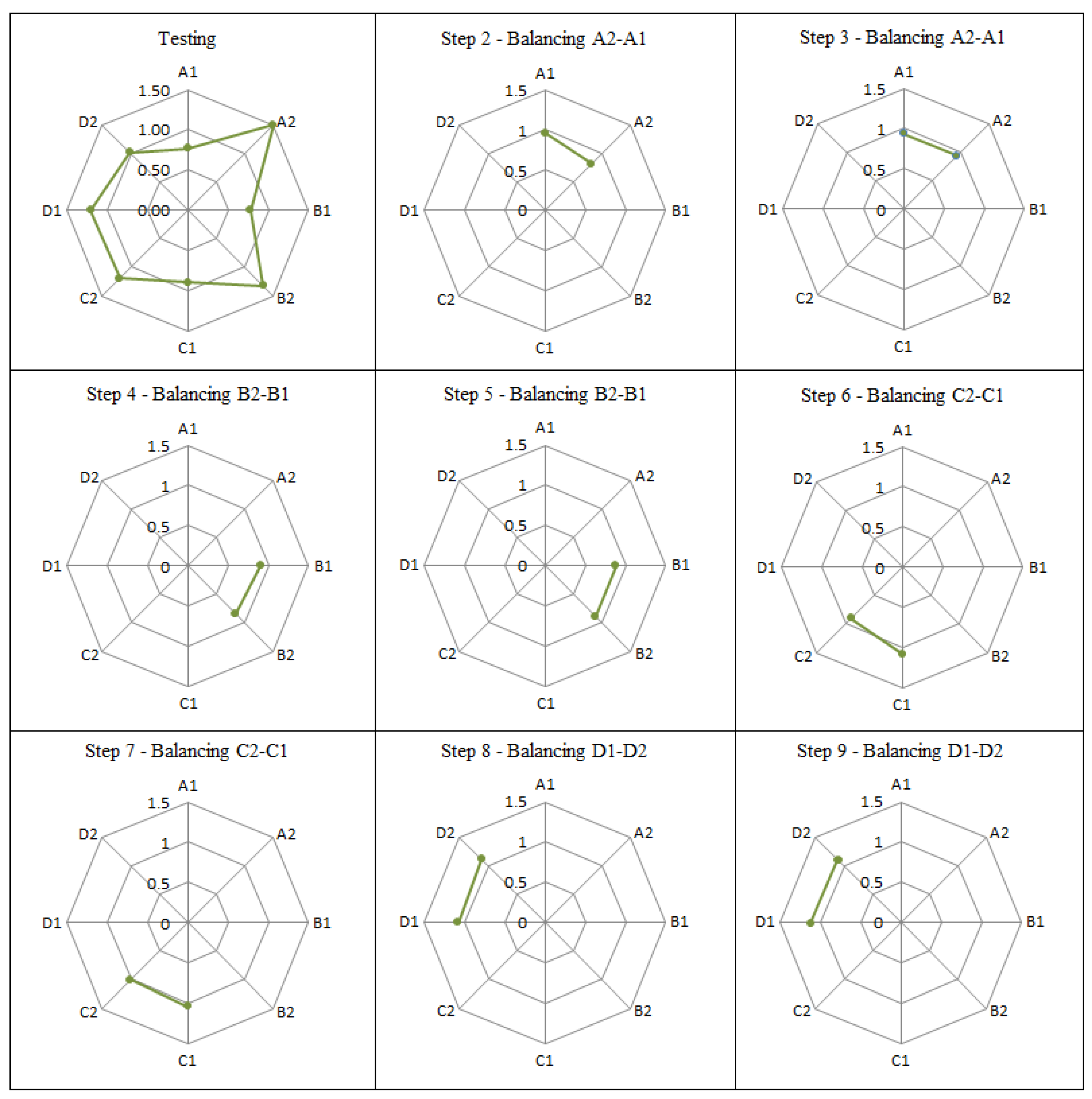
Appendix F.2. Application of the Progressive Flow Method (PFM) Procedure

The PFM method was then applied according to the proposed procedure as shown in Figure A11. Since there are only two terminals for each branch, it is irrelevant whether they are connected to a zone manifold or, as in the case tested, derived from a tee; in both cases they will be referred to the same pressure. To be able to determine which terminal is the unfavorable without reading of terminal probes (actually available in the test rig but not supposed to be used by PFM procedure), the procedure indicates to run the pump at a constant speed, open one terminal at a time, measure the flow rate via the rotameter at the pump, and sort the users according to the ratio of the measured flow rate vs the nominal flow rate.
Figure A11. PFM TAB sequence; testing and terminal balancing.
Applsci 14 06232 g0a11
In Figure A11—Testing, the flow measurement taken at the terminals using the MBV probes (not supposed to be used with the PFM) is shown for the sole purpose of verifying that the starting configuration with all valves fully open is the same for both methods tested. The method then proceeds as per procedure (Figure A12 Steps from 2 to 9), for each zone (with all other zones closed acting on branch valves), the reference terminal is fully opened and brought directly to its nominal flow rate (as measured by the rotameter at the pump) by acting on the inverter and/or the bypass branch; then the reference loop pressure control is activated, and the other terminal is progressively opened until the two terminals’ summed flow rate is measured by the rotameter at the pump according to the concept of flow rate progressivity.
Afterwards, the operator moves on to the next branch and so on; unlike the RM procedure, in this case there is no iteration, and each terminal can be brought exactly to its nominal flow rate according to the resolution of the instrument. For terminals balancing, the rotameter activated is the smaller, more suitable in terms of range and resolution.
Once the balancing of the terminals branch by branch is complete, the operator moves on to the balancing of branches (Figure A12).
Figure A12. PFM TAB sequence; testing and branches balancing.
Applsci 14 06232 g0a12
All branches are closed except for the most disadvantaged one (branch A), which is brought up to nominal flow rate, the reference control is activated, and branches C, B, and D are progressively opened, again without iteration. This time the rotameter considered is the one with the higher range, which is more suitable in terms of flow values and resolution for balancing branches.
Finally, adjusting is not required since the right pump speed is intrinsically achieved by the reference control loop along the procedure of branches balancing.
The final result is shown in Figure A12—step 12, the values reported are measured in terms of the progressive increase in flow rate at the rotameter during the progression of the procedure and incorporate the 10% tolerance level accepted at each step within the limits of the instrument’s resolution. The number of measuring actions related to the virtual moving pressure gauge from one terminal to another is only required by the setting of the reference control, and in the current case it counts one each for the four branches and one for the final balancing of branches, so Nmeas= 1 × 4 + 1 = 5. Regarding the number of balancing operations, the procedure requires one operation per terminal and then one per branch, so Nbal = 8 + 4 = 12.

References

  1. Directive (EU) 2024/1275 of The European Parliament and of the Council on Energy Performance of Buildings—EPBD; EUR: Rome, Italy, 2024.
  2. ISO/TC 205, CEN/TC 247, ISO 52120-1:2021; Energy Performance of Buildings—Contribution of Building Automation, Controls and Building Management. Part 1: General Framework and Procedures. ISO: Geneva, Switzerland, 2022.
  3. Taylor, S.T.; Stein, J. Balancing variable flow hydronic systems. ASHRAE J. 2002, 44, 17–24. [Google Scholar]
  4. Cholewa, T.; Siuta-Olcha, A.; Balaras, C.A. Actual energy savings from the use of thermostatic radiator valves in residential buildings—Long term field evaluation. Energy Build. 2017, 151, 487–493. [Google Scholar] [CrossRef]
  5. Zhang, L.; Xia, J.; Thorsen, J.E.; Gudmundsson, O.; Li, H.; Svendsen, S. Method for achieving hydraulic balance in typical Chinese building heating systems by managing differential pressure and flow. Build. Simul. 2017, 10, 51–63. [Google Scholar] [CrossRef]
  6. Sarran, L.; Smith, K.M.; Hviid, C.A.; Rode, C. Grey-box modelling and virtual sensors enabling continuous commissioning of hydronic floor heating. Energy 2022, 261, 125282. [Google Scholar] [CrossRef]
  7. Fine, J.P.; Touchie, M.F. A grouped control strategy for the retrofit of post-war multi-unit residential building hydronic space heating systems. Energy Build. 2020, 208, 109604. [Google Scholar] [CrossRef]
  8. Khamesi, S.S.; Yousefi, H.; Behrouz, B. The Effect of Flow Balance on the Reduction of Life Cycle Cost in Hydronic Networks. J. Energy Manag. Technol. 2024, 8, 93–103. [Google Scholar]
  9. Henze, G.P.; Floss, A.G. Evaluation of temperature degradation in hydraulic flow networks. Energy Build. 2011, 43, 1820–1828. [Google Scholar] [CrossRef]
  10. Averfalk, H.; Werner, S. Essential improvements in future district heating systems. Energy Procedia 2017, 116, 217–225. [Google Scholar] [CrossRef]
  11. Zhang, L.; Gudmundsson, O.; Thorsen, J.E.; Li, H.; Li, X.; Svendsen, S. Method for reducing excess heat supply experienced in typical Chinese district heating systems by achieving hydraulic balance and improving indoor air temperature control at the building level. Energy 2016, 107, 431–442. [Google Scholar] [CrossRef]
  12. Wang, H.; Wang, H.; Zhu, T. A new hydraulic regulation method on district heating system with distributed variable-speed pumps. Energy Convers. Manag. 2017, 147, 174–189. [Google Scholar] [CrossRef]
  13. Ashfaq, A.; Ianakiev, A. Investigation of hydraulic imbalance for converting existing boiler based buildings to low temperature district heating. Energy 2018, 160, 200–212. [Google Scholar] [CrossRef]
  14. Che, Z.; Sun, J.; Na, H.; Yuan, Y.; Qiu, Z.; Du, T. A novel method for intelligent heating: On-demand optimized regulation of hydraulic balance for secondary networks. Energy 2023, 282, 128900. [Google Scholar] [CrossRef]
  15. Bava, F.; Furbo, S. A numerical model for pressure drop and flow distribution in a solar collector with U-connected absorber pipes. Sol. Energy 2016, 134, 264–272. [Google Scholar] [CrossRef]
  16. Gomariz, F.P.; López, J.M.C.; Muñoz, F.D. An analysis of low flow for solar thermal system for water heating. Sol. Energy 2019, 179, 67–73. [Google Scholar] [CrossRef]
  17. De Rosa, R.; Romagnuolo, L.; Frosina, E.; Belli, L.; Senatore, A. Validation of a Lumped Parameter Model of the Battery Thermal Management System of a Hybrid Train by Means of Ultrasonic Clamp-On Flow Sensor Measurements and Hydronic Optimization. Sensors 2023, 23, 390. [Google Scholar] [CrossRef] [PubMed]
  18. Hámori, S.; Kalmár, F. Hydraulic balancing analysis of a central heating system with constant supply temperature. Environ. Eng. Manag. J. 2014, 13, 2789–2795. [Google Scholar] [CrossRef]
  19. Ryu, S.-R.; Rhee, K.-N.; Yeo, M.-S.; Kim, K.-W. Strategies for flow rate balancing in radiant floor heating systems. Build. Res. Inf. 2008, 36, 625–637. [Google Scholar] [CrossRef]
  20. Cho, H.-I.; Cabrera, D.; Patel, M.K. Estimation of energy savings potential through hydraulic balancing of heating systems in buildings. J. Build. Eng. 2020, 28, 101030. [Google Scholar] [CrossRef]
  21. Cho, H.; Cabrera, D.; Patel, M.K. Identification of criteria for the selection of buildings with elevated energy saving potentials from hydraulic balancing-methodology and case study. Adv. Build. Energy Res. 2022, 16, 427–444. [Google Scholar] [CrossRef]
  22. Cholewa, T.; Balen, I.; Siuta-Olcha, A. On the influence of local and zonal hydraulic balancing of heating system on energy savings in existing buildings—Long term experimental research. Energy Build. 2018, 179, 156–164. [Google Scholar] [CrossRef]
  23. Petitjean, R. Total Hydronic Balancing, 3rd ed.; Tour & Andersson AB: Ljung, Sweden, 2012. [Google Scholar]
  24. Magyar, Z. Hydronic balancing in theory and practice. In Proceedings of the 7th REHVA World Congress, Naples, Italy, 15–18 September 2001; pp. 45–53. [Google Scholar]
  25. CIBSE Commissioning Code W. Chapter 7—Balancing and regulating water flow rates. In Water Distribution Systems; CIBSE (Chartered Institution of Building Services Engineers): London, UK, 2010. [Google Scholar]
  26. Pedranzini, F.; Colombo, L.P.M.; Joppolo, C.M. A non-iterative method for Testing, Adjusting and Balancing (TAB) air ducts systems: Theory, practical procedure and validation. Energy Build. 2013, 65, 322–330. [Google Scholar] [CrossRef]
  27. Tamminen, J.; Ahonen, T.; Ahola, J.; Hammo, S. Fan pressure-based testing, adjusting, and balancing of a ventilation system. Energy Effic. 2016, 9, 425–433. [Google Scholar] [CrossRef]
  28. Std.111/2008; Measurements, Testing, Adjusting and Balancing of Building HVAC Systems. ANSI/ASHRAE: Peachtree Corners, GA, USA, 2008.
  29. NEBB. Procedural Standard for Testing, Adjusting and Balancing of Environmental Systems, 8th ed.; NEBB: Gaithersburg, MD, USA, 2015. [Google Scholar]
  30. American Society of Heating Refrigerating and Air-Conditioning Engineers Inc. (ASHRAE). ASHRAE Handbook—FUNDAMENTALS; ASHRAE: Peachtree Corners, GA, USA, 2021. [Google Scholar]
  31. Sugarman, S.C. Water Balance Procedures. In Testing and Balancing HVAC Air and Water Systems; The Fairmont Press: Atlanta, GA, USA, 2014; pp. 2023–2024. Available online: http://ebookcentral.proquest.com/lib/polimi/detail.action?docID=3239082.https://ebookcentral.proquest.com/lib/polimi/detail.action?docID=3239082 (accessed on 9 January 2023).
  32. ASHRAE. Chapter 39—Testing, Adjusting and Balancing. In ASHRAE Handbook—HVAC Applications; American Society of Heating: Atlanta, GA, USA, 2023. [Google Scholar]
  33. BSRIA. BBG02/10—Commissioning Water Systems; BSRIA: Berkshire, UK, 2010. [Google Scholar]
Figure 1. Compensated method procedure performed by an operator; different levels of gray indicate sequential operations, darker means more recent.
Applsci 14 06232 g001
Figure 2. Equivalence of graphical representation air vs. water system: both can be represented by the same lumped-parameters model.
Applsci 14 06232 g002
Figure 3. Representation of a hydronic distribution system at the generic shunt point.
Applsci 14 06232 g003
Figure 4. Lumped-parameters representation of a hydronic distribution system at the farthest terminal.
Applsci 14 06232 g004
Figure 5. Lumped-parameters representation of the downstream part of the circuit; for clarity, the real configuration on the left and its equivalent configuration on the right are enclosed within the dashed rectangular shapes.
Applsci 14 06232 g005
Figure 6. Insertion of a line-balancing device downstream of the disadvantaged terminal, lumped-parameters model.
Applsci 14 06232 g006
Figure 7. Insertion of a line-balancing device downstream of the disadvantaged terminal, system equipment representation.
Applsci 14 06232 g007
Figure 8. Representation of the system to be balanced, balancing devices, and required measuring points/instruments.
Applsci 14 06232 g008
Figure 9. First step of PFM procedure; tuning flow rate of the farthest terminal by adjusting pump velocity.
Applsci 14 06232 g009
Figure 10. Implementing the reference pressure loop control (second step), then acting in sequence on terminal valves from n − 1 to 1 (third step).
Applsci 14 06232 g010
Figure 11. Configuration of the system to be balanced.
Applsci 14 06232 g011
Figure 12. Test rig realization.
Applsci 14 06232 g012
Figure 13. Final valve configurations after application of ratio and PF methods.
Applsci 14 06232 g013
Figure 14. Behavior of flow rate variation vs. valve opening in a real system at different authority percentages.
Applsci 14 06232 g014
Table 1. Measurement Equipment, Models, Ranges, and Accuracies.
InstrumentModelMeasuring RangeAccuracy
Ultrasonic flow meters at terminalsBelimo electronic valves mod. EP015R0–1200 L/h6% of the reading value ranging from 25% to 100% of the measuring range.
Rotameter flow meters at the pumpFrank mod. M35050 ÷ 500 L/h8% of measured value for flow rates between 20% and 100% of measuring range according to VDE/DIN 3531.
300 ÷ 3000 L/h
Pressure probesThermokon mod. DPL1V0 ÷ 1 BarDeclared accuracy 1%, resolution 0.2 kPa.
Table 2. Design flow rates and drop simulation valves setup.
BranchTerminal UnitH/C CapacityUser ΔPFlow RateTU Valve Position
[W][kPa]l/hl/sReference
AA1114929.212000.060.6
A217245.013000.083
BB117245.013000.083
B220116.823500.103
CC114376.512500.072.5
C222995.544000.113.5
DD117245.013000.083
D228745.955000.144
Table 3. Comparison of results between RM and PFM procedures.
Design DataRatio MethodProgressive Flow Method
Terminal
Unit
Design
Flow Rate
[l/h]
Valve
Opening
[%]
Final
Pump
Speed
Flow Rate
Sum of MBV [l/h]
Valve
Opening
[%]
Final
Pump
Speed
Flow Rate
Rotameter
[l/h]
A1200100%85%2622100%80%2600
A230055%60%
B1300100%100%
B235056%70%
C1250100%100%
C240075%92%
D130073%70%
D2500100%100%
Total2600--
Table 4. Comparison between Ratio Method and Progressive Flow Method applied on the test rig.
NRatio MethodPFMDifference
Nmeas2714−48%
Nbal2213−41%
Disclaimer/Publisher’s Note: The statements, opinions and data contained in all publications are solely those of the individual author(s) and contributor(s) and not of MDPI and/or the editor(s). MDPI and/or the editor(s) disclaim responsibility for any injury to people or property resulting from any ideas, methods, instructions or products referred to in the content.

