Rule-Based DSL for Continuous Features and ML Models Selection in Multiple Sclerosis Research

Abstract

Machine learning (ML) has emerged as a powerful tool in multiple sclerosis (MS) research, enabling more accurate diagnosis, prognosis prediction, and treatment optimization. However, the complexity of developing and deploying ML models poses challenges for domain experts without extensive programming knowledge. We propose a novel domain-specific language (DSL) that simplifies the process of selecting features, choosing appropriate ML models, and defining training rules for MS research. The DSL offers three approaches: AutoML for automated model and feature selection, manual selection for expert-guided customization, and a customizable mode allowing for fine-grained control. The DSL was implemented and evaluated using real-world MS data. By establishing task-specific DSLs, we have successfully identified workflows that enhance the filtering of ML models and features. This method is crucial in determining the T2-related MRI features that accurately predict both process speed time and walk speed. We assess the effectiveness of using our DSL to enhance ML models and identify feature importance within our private data, aiming to reveal the relationships between features. The proposed DSL empowers domain experts to leverage ML in MS research without extensive programming knowledge. By integrating MLOps practices, it streamlines the ML lifecycle, promoting trustworthy AI through explainability, interpretability, and collaboration. This work demonstrates the potential of DSLs in democratizing ML in MS and paves the way for future research in adaptive and evolving DSL architectures.

1. Introduction

In the evolving landscape of contemporary healthcare, the emergence of ML signifies a pivotal change, reshaping diagnostic, therapeutic, and predictive approaches to enhanced precision and individualized patient care [1]. This technological shift not only streamlines medical processes but also fosters earlier detection, tailored treatments, and improved accuracy, setting a new benchmark for healthcare efficacy. In the field of MS research and treatment, ML has emerged as a powerful research method to address challenges such as diverse treatment responses and the often ambiguous early-stage symptoms. By leveraging early intervention and refining therapeutic approaches in MS, ML can improve diagnosis accuracy and enhance patient care. This is crucial in addressing issues related to misdiagnosis, and it lays the groundwork for individualized personalized medicine [2]. To enhance accuracy, it is essential to incorporate a wide range of features from various domains, including MRI metrics like T2 lesion size, count, and volume [3], as well as clinical data such as the Expanded Disability Status Scale (EDSS) [4] and functional tests such as walking tests [5]. Moreover, the complexity of MS, characterized by a multitude of features and variables, poses a significant challenge in feature selection. Additionally, the optimal configuration and selection of ML models are critical to achieving accurate and reliable predictions; a task that is further complicated by the diversity of patient responses and the dynamic nature of the disease.

Several studies have investigated the application of ML in the context of MS. For instance, one study employed support vector machines (SVMs) to forecast lesion data [6], while another utilized decision trees (DTs) to predict disease progression based on clinical data [7]. Given privacy concerns, the majority of medical ML research relies on sensitive data. Additionally, these studies employ varying features and ML models tailored to specific objectives. For domain experts, choosing the right features and ML models to meet their unique objectives proves challenging. Hence, we propose the creation of a DSL as a lightweighted access to defining custom logical rules to select pertinent features and determine the optimal ML model for training. Moreover, with the goal of assisting experts in identifying the results that best align with their expectations, it is advisable to design the system to automatically monitor outcomes and initiate actions based on predefined rules. These actions may include retraining a specific ML model using different features and parameters.

To construct transparent AI in MS, it is imperative to tackle the intricate relationship between ML models, data quality, and clinical workflows. By incorporating features that emphasize explainability, interpretability, data provenance, security, and facilitate collaboration between ML experts and domain specialists, the DSL can facilitate the development of accessible AI solutions in healthcare. Furthermore, as the landscape of AI and ML continues to evolve, ongoing research and development are essential to keep DSL effective, meeting the evolving demands of domain experts and patients. The DSL offers a specialized programming framework and syntax aimed at simplifying and standardizing the creation, deployment, and management of ML models. It incorporates additional concepts, including MLOps, to enhance the process. MLOps, an abbreviation for ML operations, integrates ML technology, data engineering, and DevOps (Software development and IT operations) to automate the complete ML lifecycle, thus enabling seamless deployment, monitoring, and maintenance of ML models in production settings [8]. Adopting MLOps practices within this framework can further enhance the reliability and scalability of AI solutions in MS, ensuring that they remain robust and adaptable to new challenges and data.

As previously discussed, domain experts encounter several challenges when attempting to utilize ML models, including the design of their own training rules, the navigation of the complexities of cross-directional features in MS, and the selection of the most appropriate ML model. Furthermore, the DSL serves as a bridge to enhance communication and improve coordination between ML experts and domain specialists. It provides a common language that both groups can understand and use effectively. For instance, neurologists can use the DSL to specify important features and training objectives using straightforward syntax. This clear specification allows ML engineers to implement the desired models and analyses without ambiguity, ensuring that the resulting ML solutions accurately reflect the domain experts’ requirements and expectations. This collaborative approach ensures that the resulting ML models are both technically sound and clinically relevant. This paper aims to contribute to the development of ML in MS by proposing a novel DSL. Our DSL is designed for these stakeholders, including MS experts and ML researchers. Each group has specific requirements:

1.

MS experts require an intuitive interface to select features and goals without deep programming knowledge. They require explainability and interpretability to validate the model’s decisions.

2.

ML researchers seek flexibility and control over model parameters and feature selection and require advanced customization options to experiment with different ML techniques and optimization strategies.

By addressing these requirements, our DSL ensures that all stakeholders can effectively contribute to the ML model development process in MS research. This paper is structured as follows: Section 2 provides an overview of the background knowledge on MS, detailing how ML has been implemented in MS and the methodology of DSL. Section 3 delves into our DSL design, presenting the meta model and illustrating how to define models in three distinct ways using examples. In Section 4, we define several models to test their results on real data and compare the outcomes. Section 5 reviews related work, and Section 6 summarizes our findings and outlines future directions for research.

2. Background

In this section, we provide background knowledge on MS and DSLs, as well as our research methodology for developing a DSL for ML model development in MS.

2.1. Multiple Sclerosis

MS is a complex and degenerative neurological disorder that primarily affects the central nervous system (CNS), which comprises the brain and spinal cord. The core pathology of MS lies in the immune-mediated attack on myelin sheaths—the insulating covers of nerve cells—leading to a disruption in the nervous system’s signal transmission capabilities, manifesting in a myriad of physical and mental symptoms [9,10,11]. A notable characteristic of MS is its prevalence among young adults, typically manifesting between the ages of 20 to 40 years, making it the most common disabling neurological disease in this age demographic [12]. The diagnosis of MS primarily revolves around the identification of lesions in the CNS using imaging techniques such as MRI, with Gadolinium-enhanced T1-weighted MRI being particularly useful in showing active lesions [9]. The Expanded Disability Status Scale (EDSS) is a fundamental tool for evaluating the progression of MS, measuring the degree of physical disability based on a neurological exam of seven functional systems and an individual’s walking ability. The progression of MS, as per the EDSS, is defined as a minimum increase in the EDSS from a baseline level, with the specifics dependent on the initial EDSS score [13]. Walking speed, gauged by the timed 25-foot walk (T25-FW), determines how fast a person with MS can walk 25 feet. It is used alongside the EDSS to evaluate disease progression and impact on daily activities and function [14]. It is notable that a significant correlation exists between EDSS scores and walking disability, reflecting how these measures provide a nuanced understanding of a patient’s mobility status and overall disease progression [15]. While there is no known cure for MS, several therapeutic strategies exist to manage the symptoms, expedite recovery post-attacks, reduce inflammatory disease activity, and slow down disease progression [9].

The prognosis of MS varies significantly among individuals; some experience a mild course with minimal disability, while others face a steadily worsening disease trajectory leading to increased disability over time [11]. Through artificial intelligence-based analysis of several disease parameters—including clinical and para-clinical outcomes, multi-omics, biomarkers, patient-related data, information about the patient’s life circumstances and plans, and medical procedures—a digital twin paired to the patient’s characteristics can be created, enabling healthcare professionals to handle large amounts of patient data. This can contribute to more personalized and effective care by integrating data from multiple sources in a standardized manner, implementing individualized clinical pathways, supporting physician–patient communication, and facilitating shared decision-making  [16]. However, the multifaceted nature of MS and its variable manifestation underline the need for continued research and evolving therapeutic strategies to ameliorate the lives of those affected. In this study, we propose a novel DSL-based method for analyzing MRI-related data along with different forms of clinical data such as walking abilities in patients with MS.

2.2. Ml in MS

ML techniques are increasingly being applied to MS research to assist with diagnosis, prognosis prediction, and disease subtype classification. ML algorithms can learn patterns from multidimensional clinical, imaging, and omics data to build predictive models with minimal human intervention. Regression models like logistic regression, linear regression, and regularized least squares are commonly used to predict MS outcomes and progression [17]. For example, logistic regression has been applied to predict conversion from a clinically isolated syndrome to MS [18]. Tree-based models like decision trees [19], random forests, and gradient boosted trees (e.g., XGBoost, LightGBM) [20] have shown strong performances for MS classification and prediction tasks. SVMs are effective for high-dimensional data and have been used for tasks like distinguishing between MS subtypes and predicting disability progression [21]. Different neural network architectures including convolutional neural networks and multi-layer perceptrons have been applied to analyzing neuroimaging data for MS diagnosis and lesion segmentation [22]. Given that these studies utilize a variety of features from different datasets, including clinical data, MRI scans, and patient reports, and that they employ various ML models, it poses a significant challenge for non-technical experts to interact with the ML systems effectively, let alone to train and optimize them appropriately [23].

2.3. Domain-Specific Language (DSL)

A DSL is a programming language or specification language designed for a particular problem domain, a specific problem representation technique, and/or a particular solution technique [24]. Unlike general-purpose languages such as Python, Java, and C++, which are versatile and applicable across a broad spectrum of applications, DSLs are specialized, focusing on specific tasks. Given their targeted nature, DSLs often include constructs that are optimized for efficient problem-solving within their designated domain. This specialization is particularly beneficial in fields like medicine, where professionals may struggle with software and ML engineering terminology. DSLs can simplify the development process, making it easier to create clear, maintainable functions and solutions. We have developed a DSL specifically for medical stakeholders, facilitating the management of data and the selection of ML models with greater ease. Furthermore, our DSL offers flexibility, enabling users to specify a broad array of models to fulfill their workflow requirements. This capability allows users to refine their choices among ML models and features, thereby streamlining the model and features selection.

3. Dsl Design

In this section, we present a DSL that is designed to support medical professionals in describing ML datasets. As discussed in Section 2, there are numerous ML models and features available, making it challenging for medical or non-technical people to select the most appropriate ones for their research. Our proposed DSL aims to provide a semantic representation of the ML process, enabling users to efficiently describe their datasets and select suitable models and features. The design is guided by key requirements ensuring its flexibility and applicability in MS research and treatment. To balance usability for domain experts with the power required for complex ML tasks, we opted for a rule-based approach to feature and model selection. This simplifies the process for non-technical users while still providing manual and customizable options for advanced users who need more control. This dual approach ensures that our DSL can cater to both novice and experienced users, making it a versatile tool for MS research. The main function of the DSL is to facilitate the selection of ML models and features by providing three distinct ways:

• AutoML [25]: The DSL can automatically select the best model and features based on a set of predefined criteria, such as accuracy or complexity. This approach saves time and effort for users who may not be familiar with ML techniques.
• Manual Selection: Users can manually select the most appropriate model and features by fine-tuning them using various parameters. This method provides more control over the selection process but requires a deeper understanding of ML concepts.
• Customizable: Users can set all these manually, providing maximum flexibility in selecting the ideal model and features for their research.

The DSL’s design incorporates several key features to enhance its functionality and user experience. It features a hierarchical structure for clear navigation, modularity for adaptability to various research scenarios, and unique identifiers for precise element reference. The system supports task-specific models, allowing researchers to tailor their approach to particular aspects of MS research. Flexible data loading capabilities enable users to easily import data from various sources, while comprehensive evaluation metrics provide thorough model assessment. We have also included mechanisms for feature selection, visualization, and handling of logical expressions, all facilitated by an auxiliary table for attribute values. MS experts can leverage this tool without extensive knowledge of ML models or programming. Their primary focus should be on identifying crucial features and defining clear objectives, such as data classification or feature relationship discovery. By utilizing AutoML methods, these experts can generate initial results efficiently. Subsequently, ML researchers can build upon these preliminary findings, refining and enhancing the models to achieve a superior performance. Our tool facilitates a streamlined ML data pipeline improvement process, accommodating users with varying levels of ML expertise. It promotes iterative enhancements through collaborative efforts among multiple stakeholders, fostering a synergistic approach to MS research and model development.

3.1. Meta Model Design

As we discussed, the design of our DSL’s meta model is guided by key requirements ensuring its flexibility and applicability in MS research and treatment. It features a hierarchical structure for clear navigation, modularity for adaptability, and unique identifiers for precise element reference. The DSL supports task-specific models, flexible data loading, comprehensive evaluation metrics, and a rule-based training approach. It also includes mechanisms for feature selection, visualization, and handling of logical expressions, all facilitated by an auxiliary table for attribute values. These requirements ensure the DSL is robust, capable of addressing complex challenges, and user-friendly.

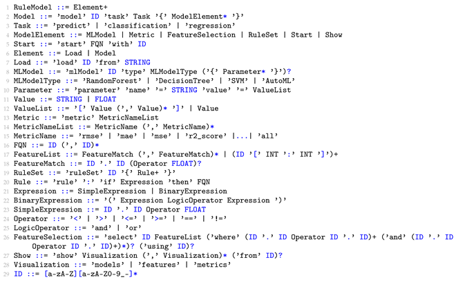
The abstract syntax of our DSL in Listing 1 defines how each construct is interpreted and executed within the context of the ML model and feature selection. Here, we provide a precise description of the key language elements:

• RuleModel: This is the root container for all the elements in a model definition. When executing a RuleModel, each contained element is interpreted and executed in sequence.
• Model: Defines an ML task with a specific name and type (classification or regression). It encapsulates all the elements required for model training and evaluation. As shown in Listing 2, the model is defined with a regression task. It includes an AutoML model, feature selection from the loaded dataset, specified metrics, visualizations, and instructions for the ML model to start with.
• Load: Specifies the data source. When executed, it loads the dataset from the specified path into memory, making it available for subsequent operations.
• MLModel: Declares a ML model type with optional parameters. When invoked, it instantiates the specified model with the given parameters.
• Metric: Defines the evaluation metrics for model performance. These metrics are calculated after model training and used in decision-making processes within rules.
• FeatureSelection: Specifies the features to be used in model training. It can include filtering conditions and feature selections. When executed, it preprocesses the dataset to include only the specified features. Listing 2 provides a comprehensive example of feature selection. This example demonstrates the ability to select multiple features from different datasets while applying specific conditions. Furthermore, for each selected feature, operators can be added to filter feature values, offering fine-grained control over the data used in the model.
• Rule: A rule is composed of two parts: the condition (expression) that checks the metrics of the ML models, and the specific action (typically selecting a model or feature set) to be taken.
• RuleSet: Contains a collection of rules for model selection and feature engineering. Rules are evaluated sequentially, and their actions are executed when conditions are met. In Listing 3, the example ruleSet contains three rules, describing a workflow for model selection and training. Initially, if the SVM model does not meet the performance criteria, the system switches to training a RandomForest model. Should the RandomForest model perform well, it is further trained with a filtered set of features. However, if the RandomForest model also underperforms, the system initiates training of a DecisionTree model with a different feature selection. This rule-based approach allows for adaptive model selection and feature refinement based on performance metrics, enabling the system to dynamically adjust its strategy to achieve optimal results.
• Start: Initiates the model training process with the specified model and feature set. It triggers the actual computation and evaluation of the ML pipeline.
• Show: Outputs the results of the model training and evaluation process. It can display model performance metrics, feature importance, or other relevant information.

Listing 1. Abstract Syntax of the DSL.

The execution flow of our DSL typically follows this sequence:

• Data are loaded using the Load statement. This step calls our defined DataManager class, which provides several functions based on pandas’ read_csv or read_sql functions depending on the data source. It can load csv, xlsx, and .db files, and it includes default data cleaning functions like handling empty features and normalization. The DataManager also handles splitting of the training and testing data, though this is applied after feature selection.
• MLModels are instantiated with their respective parameters. Each model type is mapped to its corresponding scikit-learn class based on the defined task, such as sklearn.svm.SVR or SVC. If multiple parameters are defined, it maps to scikit-learn’s grid search functionality. The special autoML model maps to either TPOTRegressor or TPOTClassifier.
• FeatureSelection is applied to select features from the dataset(s). It can select from multiple loaded datasets, combine different features from various datasets, and apply filters to the data. After feature selection, the DataManager functions are used to split the data into training and test sets.
• Metrics are calculated to evaluate model performance, mapping to functions in sklearn.metrics. Our system logs all parameters and training results in MLflow [26], which can be retrieved when checking defined rules and generating visualization diagrams.
• RuleSets and Rules are evaluated, potentially altering the model or feature selection based on the defined rules. This is implemented as conditional statements in Python, evaluating metrics and executing corresponding actions.
• The Start command initiates the training process of MLModels, including training and fitting, and it logs the corresponding results in MLflow.
• Finally, the Show command displays the results of the process. We use Matplotlib to visualize the logged results.

The proposed DSL provides a structured framework for defining and executing ML workflows in MS research. It offers clear semantics for model definition, feature selection, and rule-based execution. The DSL supports both automated and manual methods, catering to users with varying expertise levels. This design enables progressive refinement of models and features, allowing domain experts to effectively utilize ML techniques without extensive programming knowledge. The rule-based system facilitates adaptive model development, promoting an iterative approach to ML in MS research. Figure A1 serves as a structural framework for our DSL design.

3.2. Task-Specific Model Instantiation

In this section, we will give example models based on our current data requirement analysis in the three ways we mentioned. Our DigiPhenoMS [27] project is a collaborative endeavor between the MS Center at the University Hospital Carl Gustav Carus Dresden and the Digital Health research group. This project aims to investigate the heterogeneous progression of MS by leveraging the extensive data collected throughout a patient’s clinical journey. MS is a complex neurological disorder that is characterized by a highly variable disease course, which differs significantly from one individual to another. Prior to the formal diagnosis of MS, patients undergo a comprehensive anamnestic assessment and a series of necessary examinations, generating a substantial amount of data. Upon confirmation of the diagnosis, further data are accumulated during subsequent treatment sessions and routine check-up appointments. Over the span of a patient’s life, a unique data trail is formed, encompassing the various stages of the clinical pathway within the healthcare system. The data collected includes MRI, motility and cognitive assessments, and neuropsychological evaluations of 1701 patients at different phases of the disease. These diverse datasets offer valuable insights that can aid domain experts in determining the relevance of specific factors and developing predictive models. Regression algorithms are employed in this research because they are well-suited for predicting continuous variables such as disease progression scores or severity measures, and they can help uncover the relationships between various features and MS outcomes, enabling a better understanding of the factors influencing the disease. We also support classification tasks; however, in this context, we focus on regression due to the specific requirements of our data. Additionally, the extensibility of DSLs allows for the easy addition of other tasks. The current scope of the DSL is limited to supporting scikit-learn [28] compatible regression models and pipelines. By focusing on scikit-learn, the DSL can leverage the extensive ecosystem of models and tools built around this library. With the extensibility of the meta model design, we aim to integrate the model with additional ML technologies and neural networks in the future. Additionally, we intend to invite medical experts to evaluate the usability and accuracy of our DSLs, with a focus on the continuous improvement of the models and validation of the results.

The first example, shown in Listing A1, showcases how to define AutoML in our real use case model. All these models could be defined in the same file and share the data loader from the load command. Here, we load the dataset from the sqlite database. Also, we support the loading of multiple datasets from csv files and databases, and we also support joint queries between them, as shown in Listing 2. This model defines an AutoMLModel task for regression, where the mlModel parameter is set to autoML, indicating the use of an automated ML algorithm. The select pst statement specifies that the initial set of features should be selected from the entire dataset about MRI and process speed time features. Additionally, the metric parameter defines the evaluation metrics to be used, such as mean squared error (mse), R-squared score (r2_score), mean absolute error (mae), and root mean squared error (rmse). Finally, the start autoML with the pst statement initiates the AutoML process with the specified initial features and shows the models and features. AutoML techniques have gained significant attention in recent years due to their ability to streamline the ML workflow and achieve competitive performance without extensive manual intervention. Here, we integrate TPOT [29], which uses genetic programming to automate the optimization of ML pipelines with techniques like feature selection, feature construction, model selection, and hyperparameter tuning. TPOT is an AutoML system that uses genetic programming to optimize ML pipelines. TPOT supports various models provided by the scikit-learn library, including linear models, support vector machines, decision trees, random forests, and ensemble methods. We could set generations and population sizes to fine tune this model.

• Generation: This parameter determines the number of iterations that the genetic algorithm will run. Each generation involves creating a new population of ML pipelines by applying genetic operations (crossover and mutation) to the best-performing pipelines from the previous generation.

  −

  A higher number of generations allows for more thorough exploration of the solution space, potentially finding better pipelines.

  −

  However, it also increases the computation time.

  −

  In our DSL, users can specify this parameter as generation = 100

• Population size: This parameter sets the number of individuals (ML pipelines) in each generation.

  −

  A larger population size increases the diversity of solutions explored in each generation.

  −

  It can lead to better results but at the cost of increased computation times.

  −

  Users can set this in our DSL as population_size=50

The genetic processes in AutoML, specifically in TPOT, involve operations like crossover (combining parts of two high-performing pipelines) and mutation (randomly altering parts of a pipeline) to evolve increasingly effective ML workflows. These processes explore various combinations of preprocessing steps, feature selection methods, and ML algorithms. As a result, AutoML can discover complex, multi-step pipelines that often outperform manually designed models, potentially including unexpected feature transformations or ensemble methods that a human data scientist might not have considered. The output typically includes the best-performing pipeline architecture, optimized hyperparameters, and performance metrics, providing users with a ready-to-use model and insights into effective feature engineering strategies for their specific dataset. This allows researchers to focus on higher-level tasks such as problem formulations and results interpretation.

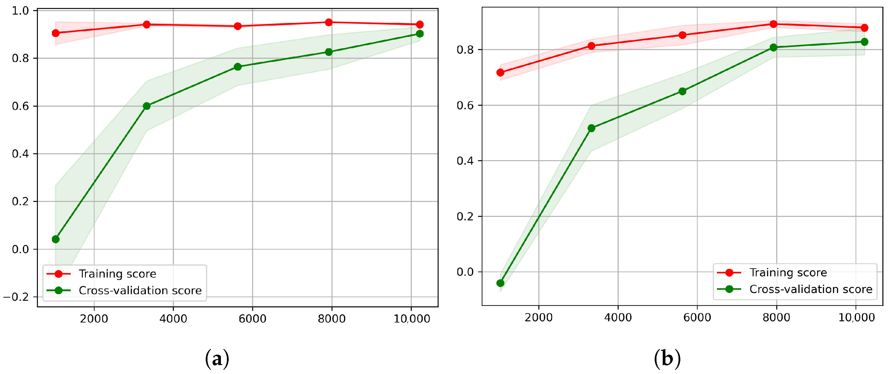
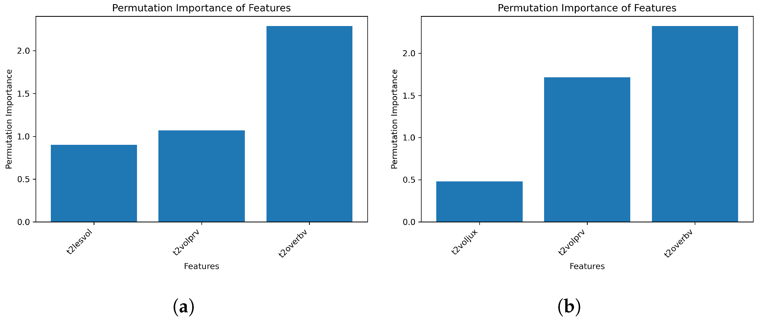
The second model, shown in Listing 3, demonstrates a manual approach to model and feature selection. In this model, three ML algorithms, random forests, decision trees, and SVMs are defined with their respective hyperparameters. The select pst statement specifies a set of initial features based on certain conditions. Additionally, a new set of features, denoted as pst_filter, is defined by utilizing a distinct dataset and specific conditions (e.g., t2lesvol > 3.0) for enhanced screening values. The ruleSet selectionRules defines a set of rules for model selection based on the evaluation metrics. If the r2_score of the SVM model is less than 0.85 and the mean squared error is greater than 0.2, the random forest model is selected. If the r2_score of the random forest model is greater than 0.8, which is a good model, then we further train it with the pst_filter features to see if it could be better. If it does not meet our expectations, we instead use a decision tree. It is worth noting that the ruleSet could also be applied to the other models; however, for the sake of brevity, only one illustrative example is presented here. The output displays the models, which presents a diagram comparing the results of two model runs, and the features, which provide a comparison of feature importance. This model showcases the manual approach to feature and model selection, where domain knowledge and expert intuition play a crucial role. This approach is suitable for further comparison screening and the comparison of customized models and features by obtaining initial results from AutoML and incorporating additional rules and conditions to fine-tune the models and features. By defining specific conditions and rules, researchers and practitioners can meticulously refine the feature selection process and systematically explore various model combinations to achieve optimal performance.

The third model, shown in Listing 4, demonstrates a customizable approach to model selection for a classification task. In this model, a decision tree algorithm is defined with specific hyperparameters, such as max_depth, min_samples_split, min_samples_leaf, and max_features. The selected pst statement specifies the most related features after verification of the last two models. Initiating the decision tree with the pst statement initiates the model training process using the specified features. This model is suitable for re-running the chosen models from coarse screening and attempting to refine them with finer granularity in terms of specific model architectures and features.

Listing 2. Model example for multiple datasets in AutoML.

Our DSL significantly enhances explainability and facilitates collaboration in MS research through its intuitive, rule-based syntax. For example, a rule like mrt_pst_17_20.t2lesvol > 2.0 is easily interpretable by clinicians, as it uses familiar clinical features and clear thresholds. In terms of collaboration, the DSL serves as a bridge between technical and clinical experts. It allows neurologists to express their domain knowledge in a format that data scientists can directly incorporate into ML pipelines. This shared language reduces miscommunication and accelerates the development of clinically relevant ML models for MS research.

The provided models showcase different approaches to model selection and feature engineering, each with its own strengths and applications. The AutoML model offers a streamlined and automated approach, while the manual selection models provide more control and flexibility for researchers and practitioners to leverage their domain knowledge and expertise. Ultimately, the choice of approach depends on the specific requirements of the problem, the available resources, and the trade-offs between automation and manual interventions. By understanding the capabilities and limitations of each approach, researchers and practitioners can make informed decisions and develop effective ML solutions tailored to their needs. The three approaches presented constitute a layered framework, allowing users to progressively refine and optimize their models according to their expertise and the level of control they desire. This framework also facilitates a better understanding of data flow through the use of more abstract and less technical language. In the following section, we will demonstrate the practical implementation and application of these models on our dataset, showcasing their performance and discussing the insights gained from each approach.

Listing 3. Model for manual selection.

Listing 4. Model for manual selection.

4. DSL Implementation and Demonstration

This research focuses on developing a DSL to streamline the process of model and feature selection for ML pipelines in the context of MS prediction and feature relationship discovery. In the Section 3, we introduced our meta model design and how to instantiate the models and features. In this section, we will show the running results and how we use this DSL to progressively obtain better results. To manage the ML lifecycle and track experiments, the DSL integrates MLflow. MLflow is an open-source platform for managing end-to-end ML workflows. It provides functionality for tracking experiments, packaging code into reproducible runs and sharing and deploying models. The DSL utilizes MLflow’s tracking APIs to log relevant information about each pipeline evaluation, such as the models used, hyperparameter values, performance metrics, and the resulting optimized pipeline. However, the design of the DSL is modular and extensible, allowing for future integration with other ML libraries and frameworks.

4.1. Training Workflows

Before proceeding, it is important to note that all the data used in this evaluation are anonymized to ensure privacy and confidentiality. Here, to evaluate the effectiveness of our DSL, we will employ it to identify the MRI features that exhibit stronger associations with motility and those that have a greater influence on cognitive abilities. Furthermore, by utilizing the historical data available, we will apply the selected models to help predict the future trajectories of patients. Based on our data collection, we aim to analyze the relationship between T2-related MRI features and patients’ walk and process speed times in the last several years. The workflow begins by employing AutoML to identify the optimal pipeline using the initial dataset from the first four years. The system logs the preprocessing steps, best models, and most relevant features. Domain experts can then refine the features, train additional ML models, and compare the outcomes. Based on a thorough evaluation, users can specify the ML model and the most crucial features and assess the predictive results. As listed in Section 3, the models can be defined as introduced. The DSL operates in a sequential manner; it commences with the AutoMLModel to log the best pipeline. Subsequently, users can define other ML models to determine if they yield improved results. With the rules predefined, the system can initiate continuous training and obtain the results. All experiments were conducted using an Acer Nitro AN515-58 laptop equipped with a 12th Gen Intel Core i7-12700H processor (2.7 GHz, 14 cores, 20 logical processors) and 16 GB of RAM. We provide the real training model definitions in Appendix B.

4.1.1. Automl

In our AutoML approach, we initially input all features to generate initial expressions and explore potential models. Our study utilized two primary datasets: the initial dataset from 2017–2020 containing 16,263 records, and a validation dataset from 2021–2023 with 12,838 records. These substantial sample sizes ensure robust model training and evaluation. The AutoML framework, implemented using TPOT’s genetic algorithm, incorporates early plausibility checks to enhance reliability. It automatically assesses data sufficiency, flagging instances where the dataset might be too small for reliable model training. Additionally, the framework monitors convergence during the training process, alerting users to potential issues such as non-convergence or overfitting. Utilizing TPOT’s genetic algorithm, we adjust the population size and generations to optimize the process. We experiment with two configurations: 30 generations and a population size of 300, as shown in line 10, as well as 10 generations with a population size of 100 line 12. Our focus is on analyzing the relationships between features related to T2 images, process speed times, and walk speed. Our DSL facilitates the reuse of definitions such as features in subsequent procedures. The results, as depicted in Figure 1, Figure 2, Figure 3 and Figure 4, showcase the performance of the models and feature importance under different configurations. we observe a typical case of overfitting in the Figure 1a: the training score (red line) starts high and remains close to 1.0 as more training examples are added in 50 min. However, the cross-validation score (green line) initially increases with more training data but then starts to decrease after reaching a peak, indicating that the model is overfitting to the training data and performing poorly on unseen data. In Figure 1b, the training score (red line) decreases slightly in 10 min as more training data are added, which is expected behavior. The cross-validation score (green line) steadily increases and converges towards the training score, suggesting that the model is learning the underlying patterns in the data without overfitting. The section model is generalizing well, and we choose this as the better result. Similarly, we perform the same analyses in Figure 3a,b. The system identifies the optimal pipeline, encompassing data preprocessing, feature selection, and a regression algorithm. For process speed time, the pipeline starts with MinMaxScaler for feature scaling, followed by SelectFwe for feature selection based on significance. A principal component analysis (PCA) with a randomized SVD solver is applied to reduce dimensionality while retaining essential information. MaxAbsScaler scales features to the range of [−1, 1] using the absolute maximum value. These preprocessing steps are logged for future use. The regression algorithm selected is KNeighborsRegressor, a non-parametric method that uses the k nearest neighbors to predict the target variable. The defined metric, the r2_score, is 0.8. For walk speed data, the pipeline incorporates decision trees, stacking, normalization, and kernel approximation techniques. The r2_score metric for this pipeline is 0.86. Our system automatically logs all the steps of the best pipeline identified by TPOT, including the pipeline’s results and all metric values defined within the DSL.

In examining feature importance, we observed minimal differences across varying generations and population sizes. However, we discovered distinct T2-related feature importance for process speed and walk speed. As depicted in Figure 2a,b and Figure 4a,b, these images illustrate the permutation importance of various features within a ML model, as defined in line 13. Permutation importance is a method that is employed to assess the relative significance of each feature in the model’s predictions. Features with higher permutation importance values are more influential in the model’s decision-making process. For process speed time, the features with the highest permutation importance are t2overbv, nt2lescn, and nt2lesgt. These features significantly impact the model’s predictions.

• t2overbv measures the ratio of T2 lesion volume to brain volume, offering an index of overall lesion burden.
• nt2lescn counts the total number of hyperintense lesions on the T2-weighted MRI.
• nt2lesgt counts the number of T2 lesions exceeding a certain size or volume.

For walk speed, the features with the highest permutation importance are t2overbv, t2lesvol, and t2volprv.

• t2lesvol measures the total volume of hyperintense lesions on the T2-weighted MRI, reflecting the overall burden of MS lesions.
• t2volprv measures the volume of T2 lesions near the ventricles.

These findings highlight the importance of T2-related features in predicting both process speed and walk speed, underscoring the need for careful consideration of these features in model development and interpretation.

4.1.2. Further Filtering of ML Models and Features

In the following section, we demonstrate how a medical expert would enhance machine learning qualities using the new DSL. By leveraging the pipeline recorded from AutoML, the system preserves the features post-preprocessing and feature engineering. This stage facilitates the provision of additional models for users to define and experiment with. Through the establishment of rules, the system can be directed to train various models and features at different times. For demonstration, we chose two prevalent models in MS research: random forests (RFs) and support vector machines (SVMs). Following the initial feature importance evaluation from AutoML, we removed less-relevant features. This stage also encompasses continuing the steps from the AutoML-derived pipeline and setting rules for training multiple models if needed. In Figure 5 and Figure 6, we depict the effects of different hyperparameters on the main test scores and feature importance for process and walk speed time by SVM. And in Figure 7 and Figure 8, we show different results training by the random forest. The optimal parameters for SVM are C = 1000 and gamma = 1.0. However, the metrics indicate that the SVM model struggles to make accurate predictions on this dataset, with metrics such as MAE = 0.628, MSE = 0.753, R2_score = 0.475, and RMSE = 0.868. n contrast, the random forest model shows improved performance, with metrics of MAE = 0.39, MSE = 0.269, R2_score = 0.813, and RMSE = 0.519, with the best parameters being n_estimators = 100 and random_state = 20. This model outperforms both the SVM and the KNeighborsRegressor obtained from AutoML. All these metrics are automatically logged by our system. Users can view them by defining visualizations in our DSL or through the webpage provided by MLflow. Additionally, these two algorithms exhibit different feature importance rankings in Figure 5a and Figure 7a. For walk speed time, the random forest model performs better than the SVM, but not as well as the decision tree model obtained from AutoML, as shown in Figure 8.

After two rounds of training, we identified the random forest model as the best ML model for predicting process speed time, with specific hyperparameters. The optimal model for predicting walk speed was the decision tree, also with specific hyperparameters. To ensure the robustness and relevance of our selected models, we aim to validate them on a dataset collected in the last three years. This validation will help us assess the models’ performance and verify if the feature importance remains consistent with our initial findings, as shown in Figure 9. On the new dataset, the logged random forest model for process speed time achieved MAE = 0.363, MSE = 0.263, R2_score = 0.853, and RMSE = 0.513. The decision tree model for walk speed time achieved MAE = 0.429, MSE = 1.096, R2_score = 0.865, and RMSE = 1.047. These results demonstrate that after our filtering workflow, the logged models maintain a high performance on the new dataset. With our DSL, domain experts can easily start with ML model and feature selection without coding knowledge. Additionally, these progressive model definitions help build the initial ML structure and aid in drawing relevant conclusions.

5. Related Work

ML is pivotal in MS research, facilitating disease progression prediction, identifying effective treatments, and personalizing patient care, thereby significantly enhancing our comprehension and management of MS. Research in this field often focuses on diagnostic classification and disease subtyping, utilizing SVMs [30] and KNNs [31] to accurately classify MS patients versus healthy controls and differentiate between MS subtypes. Another critical application of ML in MS is predicting disease progression and treatment response, with studies employing ML models to forecast the transition from relapsing–remitting MS to secondary progressive MS and to predict disability progression using data from motor-evoked potentials and other biomarkers [21,32]. These studies often integrate various data sources, including clinical [23], genetic [33], and imaging data [34], to develop multimodal and accurate predictive models. However, the complexity of these research endeavors can be daunting for domain experts without basic ML knowledge. Some studies offer DSLs by simplifying the construction of ML workflows, as evidenced by research describing ML datasets [35], measuring and mitigating biases in ML models [36], and automating the ML pipeline [37]. While these methods enhance the engineering of ML workflows, there remains a utilization threshold for non-software-related domain experts to construct and filter ML models and features. Our research aims to bridge this gap by providing clear and concise syntax to facilitate training based on existing knowledge and offering an incremental process to discover optimal solutions.

6. Conclusions

This paper presents a novel DSL designed to assist medical professionals and domain experts in developing and deploying ML models for multiple sclerosis research. The DSL offers three approaches—AutoML, manual model selection, and customizable model configuration—enabling users to choose the most appropriate method and improve the results iteratively based on their expertise and requirements. The AutoML approach leverages genetic programming to automatically explore and optimize ML pipelines, reducing the need for manual intervention. The manual selection method allows experts to define specific models, features, and rules, providing greater flexibility and control. The customizable approach enables fine-tuning of model architectures and hyperparameters, catering to advanced users seeking maximum customization. The DSL was implemented and evaluated using real-world multiple sclerosis data, demonstrating its effectiveness in identifying relevant features, selecting optimal models, and predicting clinical outcomes such as process speed time and walk speed. The results highlight the importance of T2-related MRI features in predicting disease progression, underscoring the DSL’s capability to uncover valuable insights from complex datasets. By integrating MLOps practices, the DSL streamlines the end-to-end ML lifecycle, enabling efficient model deployment, monitoring, and maintenance performed by base technology like MLflow. The proposed DSL represents a significant step towards democratizing ML in the MS domain, empowering medical professionals and researchers to leverage the power of AI without extensive programming knowledge. In the future, we aim to expand the current DSL to incorporate neural network and unsupervised learning algorithms. We aim to incorporate data preprocessing and feature engineering guidance directly into the DSL, thereby improving the ability of domain experts to manage data more effectively. Moreover, the meta model of DSL can serve as a foundation to streamline the creation of more specialized DSLs tailored to various medical use cases and the specific requirements of different domains. This process of DSL construction can be automated and enhanced by AI technologies, enabling the system to be optimized incrementally.