A Method for Predicting Indoor CO₂ Concentration in University Classrooms: An RF-TPE-LSTM Approach

Abstract

Classrooms play a pivotal role in students’ learning, and maintaining optimal indoor air quality is crucial for their well-being and academic performance. Elevated CO₂ levels can impair cognitive abilities, underscoring the importance of accurate predictions of CO₂ concentrations. To address the issue of inadequate analysis of factors affecting classroom CO₂ levels in existing models, leading to suboptimal feature selection and limited prediction accuracy, we introduce the RF-TPE-LSTM model in this study. Our model integrates factors that affect classroom CO₂ levels to enhance predictions, including occupancy, temperature, humidity, and other relevant factors. It combines three key components: random forest (RF), tree-structured Parzen estimator (TPE), and long short-term memory (LSTM). By leveraging these techniques, our model enhances the predictive capabilities and refines itself through Bayesian optimization using TPE. Experiments conducted on a self-collected dataset of classroom CO₂ concentrations and influencing factors demonstrated significant improvements in the MAE, RMSE, MAPE, and R². Specifically, the MAE, RMSE, and MAPE were reduced to 2.96, 5.54, and 0.60%, respectively, with the R² exceeding 98%, highlighting the model’s effectiveness in assessing indoor air quality.

1. Introduction

The National Human Activity Pattern Survey (NHAPS) showed that respondents spent an average of 87% of their time in enclosed buildings, while the remaining 6% was spent in cars and 7% outdoors [1]. Indoor air pollutants (such as CO₂ and HCHO) can be harmful to human health, leading to drowsiness, headaches, or reduced concentration [2]. The primary indoor activity area for students is the classroom. Previous studies have shown that indoor air quality in classrooms affects students’ learning efficiency and concentration and may also have long-term effects on the physical health of both students and teachers [3,4]. Poor indoor air quality can increase student absences, decrease test scores, and even cause people to develop sick building syndrome [5,6,7]. Ramalho et al. [8] showed, through measurements, that indoor CO₂ levels are a good indicator for investigating air pollutants in classrooms. The Hygienic Standard for Carbon Dioxide Indoor Air states that the standard for indoor CO₂ concentration is 1000 ppm [9]. Allen et al. [10] noted through controlled experiments on the threshold standard for CO₂ concentration (500 ppm to 1500 ppm) that both high and low CO₂ concentrations have an impact on people’s health and productivity. Additionally, Zhang et al. [11] showed that working in a room with CO₂ at a high concentration of 5000 ppm leads to physical and psychological discomfort, as well as a decrease in cognitive performance. Moreover, it was found that students’ task performance speed, test scores, and attendance increased when the CO₂ concentration decreased [12,13]. A prevalent approach to managing indoor CO₂ concentrations is through ventilation [14]. However, there are identified ventilation shortcomings in American educational institutions [15]. Assessing the necessity of activating the ventilation system preemptively to address classroom CO₂ levels poses a significant challenge. Therefore, predicting CO₂ concentrations in classrooms is necessary to create a comfortable learning environment for students. Predicting CO₂ concentrations with high accuracy can provide valuable data to support corresponding ventilation measures in classrooms.

Numerous scholars have explored various approaches for predicting indoor CO₂ concentrations. One popular approach for making these predictions in classroom environments relies on traditional mathematical or physical principles. Luther et al. [16] employed a mass balance equation to create a dynamic calculator that visualizes the impact of the indoor volume, exhalation rate, air exchange rate, carbon dioxide exhalation rate, and initial CO₂ concentration in the environment on the accumulation and decay of CO₂ in a room. Teleszewski et al. [17] developed an integrated equation based on factors such as the initial CO₂ concentration, air exchange rate, per capita occupancy, and CO₂ exhalation rate for individuals engaged in different activity intensities. The proposed model has the potential to be used when analyzing indoor air quality. Yalcin et al. [18] controlled variables such as the number of students, physical characteristics, and activity intensity in a faculty building at Sakarya University to validate their developed mathematical model and simulator software. This software can be used to analyze the variation in CO₂ concentration under different indoor conditions considering factors such as various ventilation methods, staffing levels, window and door properties, and room shapes and sizes. Choi et al. [19] utilized a double exponential smoothing model to predict CO₂ emissions in 50 states and in the U.S. transportation sector and showed that this model is supported by validity tests for pseudo out-of-sample predictions. Traditional prediction methods such as trend extrapolation models, time series models, and multivariate linear regression models perform well when handling original data and exhibit a clear linear relationship. However, these methods have limitations when addressing nonlinear relationships between indoor CO₂ emissions and their influencing factors. Deep learning has gained popularity in predicting environmental states or data because it can extract complex, high-level hidden information from large high-dimensional datasets. Xiang et al. [20] applied the least absolute shrinkage and selection operator (LASSO) regression and whale optimization to optimize the nonlinear parameters, and Mardani et al. [21] used dimensionality reduction, clustering, and machine learning algorithms to predict the impact of energy consumption and economic growth on CO₂ emissions. Their study involved clustering the data, reducing the dimensionality via singular value decomposition, and constructing CO₂ prediction models via an adaptive fuzzy inference system and artificial neural networks for each cluster in the self-organizing map. Ahmed et al. [22] studied the effects of energy consumption, financial development, gross domestic product, population, and renewable energy on CO₂ emissions. They employed long short-term memory (LSTM) [23] to evaluate the impact of these factors on CO₂ emissions. Qader et al. [24] employed a nonlinear autoregressive (NAR) neural network, Gaussian process regression (GPR), and the Holt–Winters seasonal method to forecast CO₂ emissions in the context of combating global warming. Jung et al. [25] conducted a comparative analysis of three deep learning neural network models, namely the artificial neural network (ANN), nonlinear autoregressive network with exogenous inputs (NARX), and LSTM, to determine the most effective model for predicting the temperature, humidity, and CO₂ concentration in greenhouses. However, the model parameters were manually selected, and multiple parameter selection adjustments aimed at further optimizing the model’s performance to a greater degree were not present. Sharma et al. [26] modified the LSTM structure by removing the forget gate to predict the CO₂ concentration and fine particulate matter (PM_2.5) concentration, both of which significantly impact the indoor air quality. They proposed the LSTM without the forget gate (LSTM-wF) prediction model, which not only enhanced the prediction performance but also reduced the model complexity in comparison to existing models. Nevertheless, they employed their own selected particles, pollutants, and meteorological parameters as model inputs without conducting a thorough screening of these environmental parameters. Their findings indicated that neural network time series nonlinear autoregressive models outperformed other approaches in terms of predicting future CO₂ concentrations.

In summary, the use of a neural network autoregressive model is suitable for predicting CO₂ concentrations, and the LSTM neural network is usually employed to construct models for addressing time series prediction problems. Nevertheless, there is still room for improvement and enhancement in terms of the prediction accuracy. Additionally, there are various factors influencing CO₂ concentrations in classroom environments. These factors can be broadly categorized into environmental design factors and indoor air quality factors, with each major factor comprising several minor factors, which may exhibit certain correlations with one another [27]. Furthermore, the number of people indoors is considered to be strongly correlated with the CO₂ concentration [28]. However, many current studies on CO₂ concentration prediction do not consider the number of people. Therefore, it is essential to compile a comprehensive set of influencing factors that may affect indoor CO₂ concentrations. This study’s preselected set of environmental factors includes the indoor population in a classroom and various other environmental considerations that may impact CO₂ concentrations. The factors included in the final set from among all of the environmental factors should be comprehensive and pivotal to effectively predict and control CO₂ concentrations in the classroom environment.

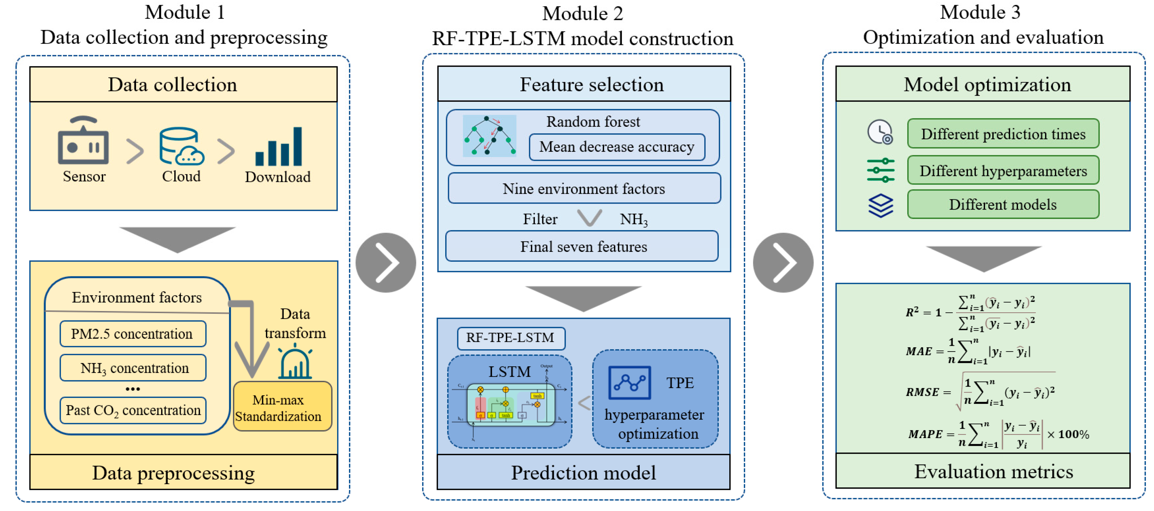
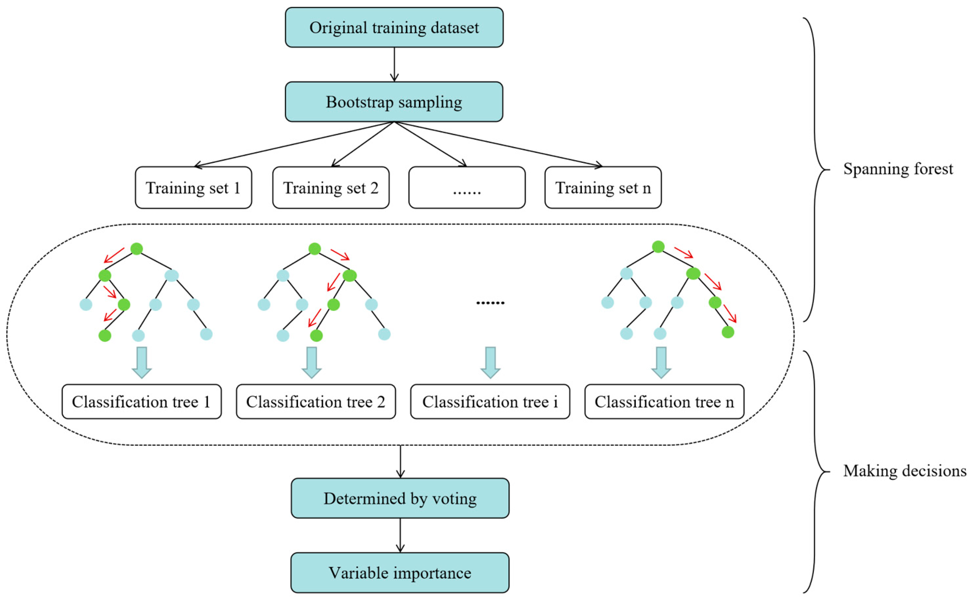
To further enhance the predictive accuracy of the LSTM network model for identifying factors influencing classroom CO₂ concentrations and to address the challenge of hyperparameter selection, which often relies on empirical experience rather than a theoretical foundation in current LSTM models, this study introduces the random forest (RF) model [29]. 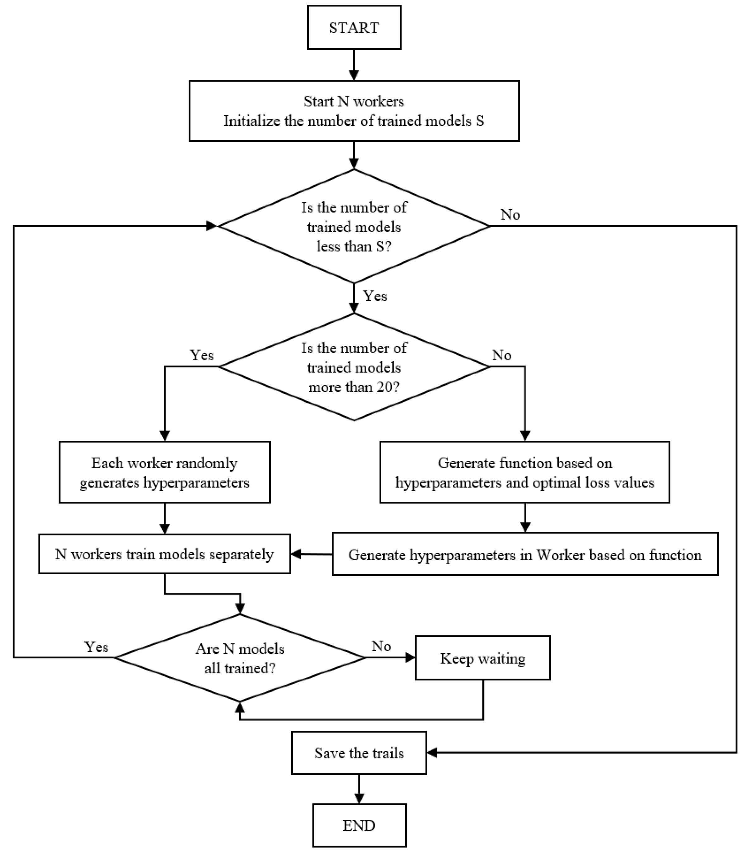The RF model was utilized to assess the significance of each environmental factor on the CO₂ concentration and subsequently rank them based on their importance. Based on the outcomes, the input variables for the LSTM model were meticulously chosen, encompassing the most pertinent influencing factors. Furthermore, the tree-structured Parzen estimator (TPE) algorithm [30] was introduced to enhance the selection of crucial hyperparameters for the LSTM model, culminating in the development of the RF-TPE-LSTM model for CO₂ concentration prediction. In the final stage of experimentation, the RF-TPE-LSTM model was compared with the RF-LSTM model, and the prediction accuracy of the RF-TPE-LSTM model was evaluated using performance metrics such as the coefficient of determination (R²) [31], mean absolute error (MAE) [32], root mean square error (RMSE) [33], and mean absolute percentage error (MAPE) [34]. The experimental results clearly demonstrated that the selection of influencing factors had a certain impact on the CO₂ concentration prediction model, and there are also different prediction effects for different prediction times. The optimized model outperformed the unoptimized model, demonstrating significant advantages in terms of predictive accuracy. The R² value achieved by the RF-LSTM model was greater than 95%, while that of the RF-TPE-LSTM model significantly surpassed this value, achieving an R² exceeding 98%. Moreover, the RF-TPE-LSTM model not only demonstrated better fitting and superior prediction accuracy compared to the RF-LSTM model but also outperformed the unoptimized LSTM model and other models. Hence, the CO₂ prediction model developed in this study proves to be highly effective at forecasting the concentration of CO₂ in indoor environments for future periods. This model provides a dynamic foundation for regulating classroom ventilation rates, thereby helping to create a healthy and productive learning environment for students.

The remainder of this paper is structured as follows: Section 2 describes the dataset used in this study, along with the constructed model. Section 3 discusses data processing and presents the results of the comparison of different prediction times, hypermeters, and models. Finally, in Section 4, a summary and future directions for predicting indoor CO₂ concentrations are provided.

2. Materials and Methods

The overall framework of this study is illustrated in Figure 1. This framework is primarily divided into three stages: In the first stage, the research status is introduced, the required data for the study are collected, and preprocessing is performed. The second stage encompasses the selection of influential factors from the data as well as the construction and optimization of the prediction model. In the third stage, our focus is on presenting the research findings while evaluating the predictive performance of the model, which involves testing various parameters and assessing the model’s efficacy across multiple experiments.

2.1. Data Collection

The data collection device used in this study was situated in a university classroom located in the central region of China. The classroom has an area of 56 m² with a length of 8 m and a width of 7 m. Classes are scheduled from 8:00 a.m. to 11:50 a.m., 2:00 p.m. to 5:50 p.m., and 6:30 p.m. to 8:10 p.m. Moreover, the classroom serves as a public study room during nonclass hours. The physical layout of the classroom is depicted in Figure 2. We installed a multi-in-one sensor at the center of the classroom one meter above the ground. This sensor is capable of measuring various environmental factors, including the temperature, humidity, illuminance, O₂ concentration, NH₃ concentration, PM_2.5 concentration, PM₁₀ concentration, and CO₂ concentration. It serves as a comprehensive data collection device for assessing the multiple factors that influence environmental comfort within the classroom. Once the sensors were linked to the host and connected to the network, various environmental data became accessible and could be viewed and exported using a cloud platform. The sensor’s data collection process is visualized in Figure 3. Figure 4 displays the specific sensors utilized in this study.

The initial experimental data used in this study were gathered from 17 October 2022, 00:00, to 30 November 2022, 24:00, with a sampling frequency of every 10 min. This dataset includes nine distinct values: temperature, humidity, illuminance, O₂ concentration, NH₃ concentration, PM_2.5 concentration, PM₁₀ concentration, past CO₂ concentration (as measured by sensors), and indoor population, as recognized by classroom cameras. The dataset is complete, devoid of anomalies, and provides detailed information for each sensor parameter, as outlined in

Table 1. Sensor parameter information.

Collection Data Type	Range	Resolution	Accuracy
Temperature (°C)	−40~+80	0.1	±0.5 °C
Humidity (%)	0~100	0.1	±3%
Illuminance (lx)	0~200,000	1	±7%
O2 concentration (% Vol)	0~30	0.1	±2%
NH3 concentration (ppm)	0~100	1	±8%
PM2.5 concentration (μm/m3)	0~1000	1	±10%
PM10 concentration (μm/m3)	0~1000	1	±10%
CO2 concentration (ppm)	0~5000	1	±3%

. Additionally, the data have been uploaded to the Supplementary Materials for further reference.

2.2. Data Preprocessing

Because of variations in the magnitudes of the different attributes within the dataset used in this study, there may be large differences in the absolute values among the data [35]. To mitigate the impact of these variations on the experimental results and to standardize the data, we applied min–max normalization [36] to nine distinct values in the initial experimental dataset. This process scales the attributes to a consistent range, ensuring uniformity in the data.

The application of min–max normalization transforms the values of each attribute to a desired range, typically $\left[0,1\right]$, facilitating attribute comparability. Min–max normalization is defined in Equation (1) as follows:

$$x^{\prime }={\displaystyle \frac{x-\min \left(x\right)}{\max \left(x\right)-\min \left(x\right)}}$$

(1)

where $x$ is the original feature and $x^{\prime }$ is the normalized feature.

2.3. Model Feature Selection

To predict the CO₂ concentration in the classroom, we gathered data on a range of environmental factors that might influence indoor CO₂ levels as the initial set of variables. However, having an excessively large number of influencing factors can lead to redundant data, increasing the complexity and time needed to develop a CO₂ concentration prediction model. Conversely, if the number of influencing factors is too limited, poor prediction outcomes may result due to an insufficient number of training samples for the model. Finding the right balance in the dimensionality of the influencing factors is crucial for an effective and accurate CO₂ concentration prediction model. The relative importance of each factor in terms of its effect on CO₂ levels can vary, and those factors with low relative significance should be excluded beforehand. Therefore, the task of selecting the most important influencing factors from the environmental factor set, identifying which factors to utilize as input variables for model training, and assigning appropriate weights to each factor are fundamental steps in data preprocessing. In this context, we employ the RF algorithm to rank the importance of preselected environmental factors. This method helps determine the strength of the relationships between variables and highlights the most influential factors when predicting CO₂ concentrations.

The RF algorithm introduces a random attribute selection process during training. Multiple rounds of sampling are performed by bagging techniques, sequentially generating decision trees for the obtained samples. These trees are subsequently combined, and the model’s output is determined through a voting technique. The RF model is an integrated prediction model comprising multiple decision tree prediction models, represented as $F=\left\{h\left(x,{\vartheta }_k\right),k=\mathrm{1,2},3,\cdots ,K\right\}$, where $\left\{{\vartheta }_k\right\}$ is an independently and identically distributed random vector and $K$ is the number of decision trees in the RF. Given an input variable $x$, the classification of $x$ is ultimately determined after multiple decision trees in the RF have been evaluated. The primary steps for constructing the RF are depicted in Figure 5.

One of the features of the RF algorithm is the estimation of feature importance for the classification problem by calculating feature importance scores, which are now widely used in feature selection and evaluation [37]. The algorithm typically employs the mean decrease accuracy (MDA) [38] to assess feature importance. The RF algorithm consists of the following eight steps:

(1)

The bag samples from the original training dataset $O=\left(X,Y\right)$ are used to obtain $M$ sets of training samples.

(2)

The decision tree ${\sigma }_1$ is trained based on sample subset $O_1$, during which the out-of-bag (OOB) sample is ${\Gamma }_1^{oob}$.

(3)

The decision tree ${\sigma }_1$ is applied to predict the OOB sample ${\Gamma }_1^{oob}$, and the number of correctly predicted samples are recorded as $R_1^{oob}$.

(4)

$d$ (where $d$ = $1,2,\cdots ,P$) features of the OOB sample ${\Gamma }_1^{oob}$ are randomly disrupted to create $P$ new OOB samples as ${\Gamma }_{1,d}^{oob}$.

(5)

The decision tree ${\sigma }_1$ is applied to predict the samples from the $P$ new OOB samples created in the previous step, and the number of correctly predicted samples is recorded as $\left\{R_{\mathrm{1,1}}^{oob},{\cdots R}_{1,d}^{oob},{\cdots R}_{1,P}^{oob}\right\}$.

(6)

Steps 2 to 5 are repeated for sample subsets $O_2,\cdots O_m,\cdots O_M$ in sequence, obtaining the number of correctly classified samples as $\left\{R_2^{oob},R_{\mathrm{2,1}}^{oob},{\cdots R}_{2,P}^{oob}\right\},\cdots ,\left\{R_M^{oob},R_{M,1}^{oob},{\cdots R}_{M,P}^{oob}\right\}$.

(7)

The importance score of the $d$th feature is calculated with Equation (2), which is defined as follows:

$$P_d={\displaystyle \frac{1}{M}}{\sum }_{m=1}^M\left(R_m^{oob}-R_{m,d}^{oob}\right)$$

(2)

(8)

The importance scores of the $P$ term features are collated.

By using the RF algorithm for the feature importance calculations related to the preselected environmental factors, the importance of each factor can be ranked. Consequently, the factors influencing the CO₂ concentration can be identified.

2.4. RF-TPE-LSTM Prediction Model Construction

To accurately predict the CO₂ concentration in classrooms, we introduce the RF algorithm described above to determine the importance of each factor and select the influencing factors as model inputs. Additionally, using the TPE algorithm to optimize the selection of hyperparameters for the LSTM model, we propose the RF-TPE-LSTM model for predicting CO₂ concentrations in classrooms.

For time series prediction tasks, such as predicting environmental parameters, most current studies employ LSTM neural networks to construct prediction models. These networks have an internal processing unit that is capable of efficiently updating and storing both backward and forward dependencies, making them suitable for accurately modeling time series data with short-term and long-term dependencies. LSTM neural networks employ three types of “gates” to control the flow of information: the forget gate, input gate, and output gate. The core structure of the LSTM neural network is depicted in Figure 6.

The forget gate decides which information is from the previous moment’s memory cell state $C_{t-1}$ and whether it should be retained as part of the current memory cell state $C_t$. The input gate determines which new information from the current moment can be incorporated into the current memory cell state $C_t$, and the output gate determines which information in the current memory cell state $C_t$ at the current moment should be saved to the current hidden layer state, $h_t,$ and subsequently output. The calculation process for these three gates is defined in Equations (3)–(8).

$$f_t=\sigma \left(W_f\cdot \left[h_{t-1},x_t\right]+b_f\right)$$

(3)

$$i_t=\sigma \left(W_i\cdot \left[h_{t-1},x_t\right]+b_i\right)$$

(4)

$$o_t=\sigma \left(W_o\cdot \left[h_{t-1},x_t\right]+b_o\right)$$

(5)

$$\widetilde{C_t}=tanh\left(W_c\cdot \left[h_{t-1},x_t\right]+b_c\right)$$

(6)

$$C_t=f_t\cdot C_{t-1}+i_t\cdot \widetilde{C_t}$$

(7)

$$h_t=o_t\cdot tanh\left(C_t\right)$$

(8)

where $f_t$ is the forget gate, $i_t$ is the input gate, $o_t$ is the output gate, $\widetilde{C_t}$ represents the temporary state entered at time $t$, $h_{t-1}$ is the output of the model at moment $t-1$, $x_t$ is the input of the model at moment $t$, $W$ represents the weight, $b$ represents the bias term, $\sigma$ denotes the sigmoid activation function, and $tanh$ denotes the tanh activation function.

The LSTM model parameters used in this study are listed in

Table 2. LSTM model parameters.

Parameter	Parameter Value
Number of input layer nodes	7
Number of hidden layers	1
Number of output layer nodes	1
Loss function	MSE
Activation function	ReLU
Optimization function	Adam

. However, the hyperparameters of the neural network have an impact on both the training speed and accuracy of the model; therefore, the hyperparameters must be adjusted to optimize the prediction accuracy of the neural network. The TPE algorithm first employs a stochastic process to generate the hyperparameters. Then, the sampled hyperparameters are utilized to evaluate the target function, resulting in a learning sample, which is denoted as $\mathrm{S}\left(x,y\right)$. In this context, $x$ represents the configuration of the hyperparameters, and $y$ denotes the optimal value achieved by applying the hyperparameter configuration $x$ to the target function. Subsequently, the acquisition function is updated based on the learning sample $\mathrm{S}\left(x,y\right)$, and the next set of hyperparameter configurations ${\lambda }_N$ is selected. This process continues until a certain number of randomly selected samples are obtained. The TPE method uses existing sample data to construct a nonparametric probability density function and samples it in the hyperparametric space to generate new learning samples. This cycle repeats until a hyperparameter configuration that yields a superior objective function value is found and recorded in each trial. In this paper, we utilized the Hyperopt optimizer to implement the TPE optimization for the LSTM model, where the number of samples randomly sampled by Hyperopt defaults was 20; the workflow is depicted in Figure 7.

2.5. Model Optimization

After conducting feature selection, eight influential factors (including the temperature, humidity, illuminance, O₂ concentration, PM_2.5 concentration, PM₁₀ concentration, indoor population, and past CO₂ concentration) were identified and utilized as input variables for the RF-TPE-LSTM model. The study involved training, validating, and testing the models on a computer with the following configuration: Ubuntu 20.04 LTS operating system, an NVIDIA RTX A4000 GPU (NVIDIA Corporation, Santa Clara, CA, USA), an Intel Xeon 4210R CPU @ 3.20 GHz processor (Intel Corporation, Santa Clara, CA, USA), and 64 GB of RAM (Kingston Technology, Fountain Valley, CA, USA). Hyperopt was employed to iteratively adjust and optimize the hyperparameters, and the model’s hyperparameter optimization ranges are shown in

Table 3. Model’s hyperparameter optimization.

Hyperparameter	Hyperparameter Range
Units	(40, 120)
Learning rate	(1 × 10−6, 1 × 10−2)
Epochs	(60, 150)
Batch size	(50, 160)
Dropout rate	(0.0, 0.2)

, ultimately achieving the optimal combination.

To assess the prediction performance of the RF-TPE-LSTM model, two aspects were considered. Firstly, in terms of the prediction time, historical 60 min data were utilized to forecast the classroom at various future time points (10, 20, 30, 40, and 50 min), with the optimal prediction time determined to be 10 min. Secondly, the RF-TPE-LSTM model was compared with state-of-the-art methods, namely, the RNN [39], BPNN [40], LSTM [23], and Optuna–LSTM [41]. Additionally, the prediction performance was evaluated both with and without the use of TPE.

2.6. Evaluation Indicators

In this study, we employed four evaluation metrics, the R², MAE, RMSE, and MAPE, to assess the performance of the overall dataset predictions. A better model fit is indicated when the R² value gradually approaches 1. The MAE characterizes the model’s credibility, with a larger value indicating poorer predictive ability and a lower value indicating better predictive ability. The RMSE is used to evaluate the deviation between the true value and the predicted value; a smaller RMSE indicates better prediction ability, while a larger value suggests worse predictive ability. A value of 0 signifies that all of the values predicted by the model are identical to the true values. The MAPE represents the actual prediction error of the model, and its value range is $\left[0,+\mathrm{\infty }\right]$. An MAPE value of 0 also implies that the predicted value exactly matches the real value. These four evaluation metrics are defined in Equations (9)–(12) as follows:

$$R^2=1-{\displaystyle \frac{{\sum }_{i=1}^n{\left({\widehat{y}}_i-y_i\right)}^2}{{\sum }_{i=1}^n{\left({\stackrel{\leftharpoonup }{y}}_i-y_i\right)}^2}}$$

(9)

$$MAE={\displaystyle \frac{1}{n}}{\sum }_{i=1}^n\left|y_i-{\widehat{y}}_i\right|$$

(10)

$$RMSE=\sqrt{{\displaystyle \frac{1}{n}}{\sum }_{i=1}^n(y_i-{\widehat{y}}_i{)}^2}$$

(11)

$$MAPE={\displaystyle \frac{1}{n}}\sum _{i=1}^n\left|{\displaystyle \frac{y_i-{\widehat{y}}_i}{y_i}}\right|\times 100\mathrm{\%}$$

(12)

where $y_i$ is the actual value, ${\widehat{y}}_i$ is the predicted value, and ${\stackrel{\leftharpoonup }{y}}_i$ is the mean of the actual data.

3. Results

3.1. Subsection Importance Analysis of Influencing Factors

In this study, we first preprocessed each collected environmental factor, which included the temperature, humidity, illumination, O₂ concentration, NH₃ concentration, PM_2.5 concentration, PM₁₀ concentration, indoor population, and past CO₂ concentration. The past CO₂ concentration data are used as an example. Figure 8 displays the experimental results of the min–max standardization, which maintain the regularity of the original data and fall within the range of $\left[0,1\right]$, meeting the requirements for data analysis and prediction. Therefore, in this study, min–max standardization was employed to transform the data for each attribute in the dataset.

As shown in Figure 9, for each of the aforementioned environmental factors, the CO₂ concentration fluctuates, which implies that individual environmental factors do not entirely predict changes in CO₂ concentration [42].

To accurately analyze the importance of each environmental factor when determining CO₂ concentrations and to filter out the influencing factors, since the past concentration has a significant effect on the current values [43], we calculated the importance of the remaining eight preselected environmental factors with respect to the CO₂ concentration via the RF algorithm, and the results are displayed in

Table 4. The relative importance of each influencing factor.

Order of Importance	Parameter	Relative Importance (%)
1	Indoor population	0.84
2	Illumination	0.54
3	PM2.5 concentration	0.44
4	PM10 concentration	0.44
5	Temperature	0.42
6	Humidity	0.39
7	O2 concentration	0.083
8	NH3 concentration	0.00059

. An analysis of Table 4 reveals that, in addition to the past CO₂ concentration, the indoor population and illumination are considered the most influential factors for the model when predicting the CO₂ concentration in the classroom environment, with relative importance values of 0.84% and 0.54%, respectively. These factors are followed in importance by the PM₁₀ concentration, PM_2.5 concentration, temperature, humidity, O₂ concentration, and NH₃ concentration, with relative importance values of 0.44%, 0.44%, 0.42%, 0.39%, 0.083%, and 0.00059%, respectively. Moreover, the other influencing factors, excluding the NH₃ concentration factor, greatly differed from the NH₃ concentration factor in their values, so these factors were retained for comprehensive analysis.

To further verify the effectiveness of the final selected influencing factors in the LSTM model, we used different numbers of environmental factors as input variables for the model performance evaluation across various indicators. The results are presented in

Table 5. LSTM performance evaluation based on different numbers of features.

Number of Features	RMSE	MAE	MAPE	R2
Top six features	21.70	18.38	3.96%	90.68%
Top seven features	14.17	7.21	1.45%	93.31%
Top eight features	15.66	9.87	2.05%	93.34%
All features	15.49	10.59	2.22%	93.38%

.

The results presented in Table 5 indicate that although selecting only the top six features (excluding the NH₃ concentration, O₂ concentration, and humidity) led to a reduction in the model’s input dimensions, it also resulted in large errors and suboptimal fitting. When all of the environmental factors were included, the model error decreased, and the fit improved to a certain extent compared to that in the previous two scenarios. However, expanding the number of input variables in the selected model also led to longer training times and increased model complexity [44]. Considering the RMSE, MAE, and MAPE, the results for the top seven features (excluding the NH₃ and O₂ concentrations) were indeed better than those for the top eight features (excluding the NH₃ concentration). However, we noted that introducing the eighth feature slightly improved the R² value of the model to more than 93%. Although the difference was not significant, it indicated that the eighth feature had a positive contribution to the model, enhancing its explanatory power and stability. While the differences between the ‘top seven features’ and ‘top eight features’ and between the ‘top eight features’ and ‘all features’ are relatively small, considering the overall performance balance, moderate complexity, model stability, and feature importance, choosing the ‘top eight features’ as the best result is reasonable and advantageous. This finding verifies that the set of influencing factors (excluding the NH₃ concentration) obtained by screening the initial environmental factors in this study is effective for the LSTM model. This approach provides experimental support when selecting input variables for the subsequent prediction of CO₂ concentrations in classrooms.

3.2. CO₂ Concentration Prediction Performance Evaluation

After analyzing the importance of the environmental factors in this study, we identified the influencing factors affecting the CO₂ concentration in classrooms and thus used the results of the RF algorithm as the input variables to the LSTM to construct the RF-LSTM model. These variables include the temperature, humidity, illuminance, O₂ concentration, PM_2.5 concentration, PM₁₀ concentration, indoor population, and past CO₂ concentration. The model’s output variable was set as the CO₂ concentration. We utilized 80% of the preprocessed final influencing factor dataset as the training set for neural network training and used the remaining 20% as the test set to assess the model accuracy [45].

As depicted in Figure 10, when the number of iterations ranged between 80 and 100, the loss function (MSE) nearly reached its minimum value, converging to approximately 0.0005. This finding suggests that the model exhibits strong convergence.

Figure 11(a1) presents the fit of the RF-LSTM model for predictions on the training set data. Subsequently, the trained and converged RF-LSTM model was used to make predictions on the test set, and the results are presented in Figure 11(b1). As shown in Figure 11(a1,b1), on the test set, the predicted values vary only slightly from the true values, and the fit is good. However, further optimization is required for the extreme values output by the RF-LSTM model for the training set and for the fitting effect in the latter part of the test set.

After multiple adjustments and optimizations of the RF-TPE-LSTM model using Hyperopt, the optimal combination of hyperparameters was determined as follows: number of LSTM units = 42, learning rate = 0.003996, number of epochs = 111, batch size = 110, and dropout rate = 0.133. Figure 11(a2,b2) show the visualization results obtained from the adjusted parameter combinations for the training and test sets, which reveal that the predicted values of the RF-TPE-LSTM model exhibit a better fit with the true values at multiple extreme points. Furthermore, the prediction accuracy does not significantly decrease in the later stages compared to that of the RF-LSTM prediction model.

Since the fitting effect is subjectively determined only by the prediction effect graph, we evaluated the prediction models for the CO₂ concentration in classrooms based on time series analysis using the four evaluation metrics mentioned earlier: MAE, RMSE, MAPE, and R².

To explore the prediction performance of the RF-TPE-LSTM model with respect to the prediction time, we used historical 60 min data to predict the classroom CO₂ concentration at multiple future time points—10, 20, 30, 40, and 50 min—with each minute representing a step. The overall evaluation of the prediction performance is shown in Figure 12, which shows that as the prediction time increases, the errors of the three evaluation indices increase to different degrees, and the R² goodness of fit gradually decreases. When predicting the classroom CO₂ concentration in the next 10 min, the lowest MAE, RMSE, and MAPE values are 2.96, 5.54, and 0.60%, respectively, and it has the best fit, with a value of 98.02% for R². When predicting the classroom CO₂ concentration for the next 30 min, the MAE, RMSE, and MAPE values increased to 10.02, 20.76, and 2.05%, respectively, while the R² decreased to 85.65%. When predicting the classroom CO₂ concentration for the next 50 min, its prediction performance is the weakest, with its MAE, RMSE, and MAPE increasing to 13.75, 28.16, and 2.73%, respectively, while its R² decreases to 73.64%. These results indicate that the RF-TPE-LSTM has good prediction ability within a certain time range, and when the prediction time is reduced, its prediction ability is better. When observing shorter historical data (from 10 min to 30 min), the model’s errors (MAE and RMSE) increase, but they still remain at a relatively low level. In particular, the MAPE values are relatively low, indicating that the model’s predictions are relatively accurate. At the same time, the R² values remain above 85%, showing that the model can explain the data variations well within a shorter time frame and has a high goodness of fit. This demonstrates that our prediction model has a high prediction accuracy and excellent explanatory power.

To verify that the TPE algorithm can optimize the selection of hyperparameters for the RF-LSTM model, we set eight different hyperparameter combinations for the RF-LSTM model and compared the accuracy with that of the RF-TPE-LSTM. The calculation results are shown in

Table 6. Prediction accuracy comparison of models with different hyperparameters.

Model	Units	Dropout	Batch Size	R2	MAE	RMSE	MAPE
RF-TPE-LSTM	42	0.133	110	98.02%	3.43	7.70	0.69%
RF-LSTM1	64	0.100	256	92.00%	9.61	15.49	2.00%
RF-LSTM2	64	0.100	128	91.52%	11.87	15.95	2.52%
RF-LSTM3	64	0.100	64	95.64%	5.26	11.44	1.06%
RF-LSTM4	64	0.100	32	83.95%	19.21	21.95	4.14%
RF-LSTM5	64	0.200	64	93.17%	10.66	14.32	2.29%
RF-LSTM6	64	0.300	64	89.38%	14.21	17.85	3.04%
RF-LSTM7	32	0.100	64	93.04%	10.25	14.45	2.16%
RF-LSTM8	128	0.100	64	91.86%	11.27	15.63	2.38%

.

To determine the effect of different batch size hyperparameters on the RF-LSTM model, we changed its batch size and set the batch sizes of the RF-LSTM1, RF-LSTM2, RF-LSTM3, and RF-LSTM4 models to 256, 128, 64, and 32, respectively. From the results in Table 6, under the same conditions as those of the other hyperparameters, the RF-LSTM3 model yields the largest R² value and the lowest MAE, RMSE, and MAPE values, indicating that different batch sizes do affect the RF-LSTM model to a certain extent.

To explore the effect of different dropout hyperparameters on the RF-LSTM model, we changed the dropout of the RF-LSTM model and set the dropout of the RF-LSTM5 and RF-LSTM6 models to 0.200 and 0.300, respectively. According to the results in the table, the RF-LSTM5 model outperforms the other models under the same conditions, confirming the need to optimize the selection of dropout hyperparameters for the models.

Finally, to determine the effect of different unit values on the LSTM model, we changed the units of the RF-LSTM model and set the units of the RF-LSTM7 and RF-LSTM8 models to 32 and 128, respectively. The results in the table show that the fitting of the RF-LSTM7 model and the error evaluation are better than those of the RF-LSTM8 model while keeping the other hyperparameters constant. This result indicates the need to improve the unit value of the RF-LSTM model.

As shown in Table 6, according to the MAE, RMSE, and MAPE metrics and compared with the RF-LSTM3, our proposed model for predicting CO₂ concentrations in the classroom, which was optimized using the TPE for the model’s hyperparameters, performs best with different hyperparameter combinations. The three error values for predicting the dataset decreased from 5.26, 11.44, and 1.06% to 3.43, 7.70, and 0.69%, which are reductions of 34.79%, 32.69%, and 34.91%, respectively. In terms of the fitting effect, the optimized RF-TPE-LSTM model achieves a larger R² value than does the RF-LSTM3 model (95.64% vs. 98.02%, respectively), which indicates that the TPE-optimized hyperparameters lead to smaller errors and a better fit to the dataset, and the RF-TPE-LSTM model returns predictions that are closer to the true values with improved accuracy. Therefore, the RF-TPE-LSTM model can be used to accurately predict CO₂ concentrations.

3.3. Comparison with Other Models

In this paper, we constructed the RF-LSTM and RF-TPE-LSTM prediction models to investigate the evolution of CO₂ concentrations in classrooms under different model applications using time series prediction hotspot research methods. To explore the generalizability of the impact of influencing factor selection on the prediction accuracy, after selecting the hyperparameters for the RF-LSTM model, we employed multiple model algorithms for comparison. We used the recurrent neural network (RNN), back-propagation neural network (BPNN), and LSTM models, along with another hyperparameter optimization framework, Optuna, to construct the Optuna–LSTM model. We trained on all the environmental factors separately. Subsequently, we adopted the RF algorithm for these models to screen the influencing factors as model inputs, resulting in the RF-RNN, RF-BPNN, RF-ARIMAX, RF-LSTM, and RF–Optuna–LSTM models. The results are shown in

Table 7. Comparison of the prediction accuracies of different models.

Model	MAE	RMSE	MAPE	R2
RNN [39]	10.27	19.94	2.17%	87.38%
BPNN [40]	11.28	18.49	0.92%	93.53%
LSTM [23]	16.70	11.73	2.49%	91.17%
Optuna–LSTM [41]	5.71	9.81	1.19%	96.79%
RF-RNN	8.50	18.55	1.79%	89.08%
RF-BPNN	8.45	15.97	0.63%	95.11%
RF-LSTM	8.27	11.71	1.78%	95.66%
RF–Optuna–LSTM	4.27	8.20	0.89%	97.76%
RF-TPE-LSTM	2.96	5.54	0.60%	98.02%

. The training results of the RF-TPE-LSTM model have been added at the end of this table for comparison.

As shown in Table 7, compared with the MAE, RMSE, MAPE, and R² values achieved using the RNN model, after constructing the RF-RNN model to screen the influencing factors, the proposed model’s error values were reduced by 17.23%, 6.97%, and 17.51%, respectively, and the goodness of fit, R², improved by 1.95%. When comparing the MAE, RMSE, MAPE, and R² values achieved using the BPNN with those achieved using the RF-BPNN model, the latter reduced the MAE by 25.01%, the RMSE by 13.63%, and the MAPE by 31.52%, respectively, while improving the R² by 1.69%. Similarly, in terms of the results of the LSTM model constructed by inputting nine feature values obtained from our previous experiments and the RF-LSTM model constructed by screening the influencing factors, the latter significantly reduced the MAE by 50.48% and the RMSE and MAPE by 0.17% and 28.51%, respectively, while improving the R² by 4.92%. Additionally, we used another hyperparameter optimization framework, Optuna, based on the LSTM algorithm, and we constructed the Optuna–LSTM and RF–Optuna–LSTM models. In terms of the training results of the two models, the latter reduced the MAE by 25.22%, the RMSE by 16.41%, and the MAPE by 25.21% while improving the R² by 1.00%.

Furthermore, among the state-of-the-art methods (RNN [39], BPNN [40], LSTM [23], and Optuna–LSTM [41]) presented in Table 7, the Optuna–LSTM achieved the best results. However, compared with the Optuna–LSTM, the proposed RF-TPE-LSTM demonstrated significantly improved performance. Specifically, it reduced the MAE by 48.16% and the RMSE and MAPE by 43.52% and 49.58%, respectively, while enhancing the R² by 1.27%.

In conclusion, the above results show that the influencing factor screening method proposed in this paper is suitable for multiple prediction models and improves the prediction accuracy of these models. These results also further validate the need to screen influencing factors. Finally, we present the RF-TPE-LSTM model proposed in this paper. The results indicate that the proposed model has the best predictive ability and the highest degree of fit, thus verifying that the RF-TPE-LSTM model we constructed has a certain degree of optimality.

4. Discussion

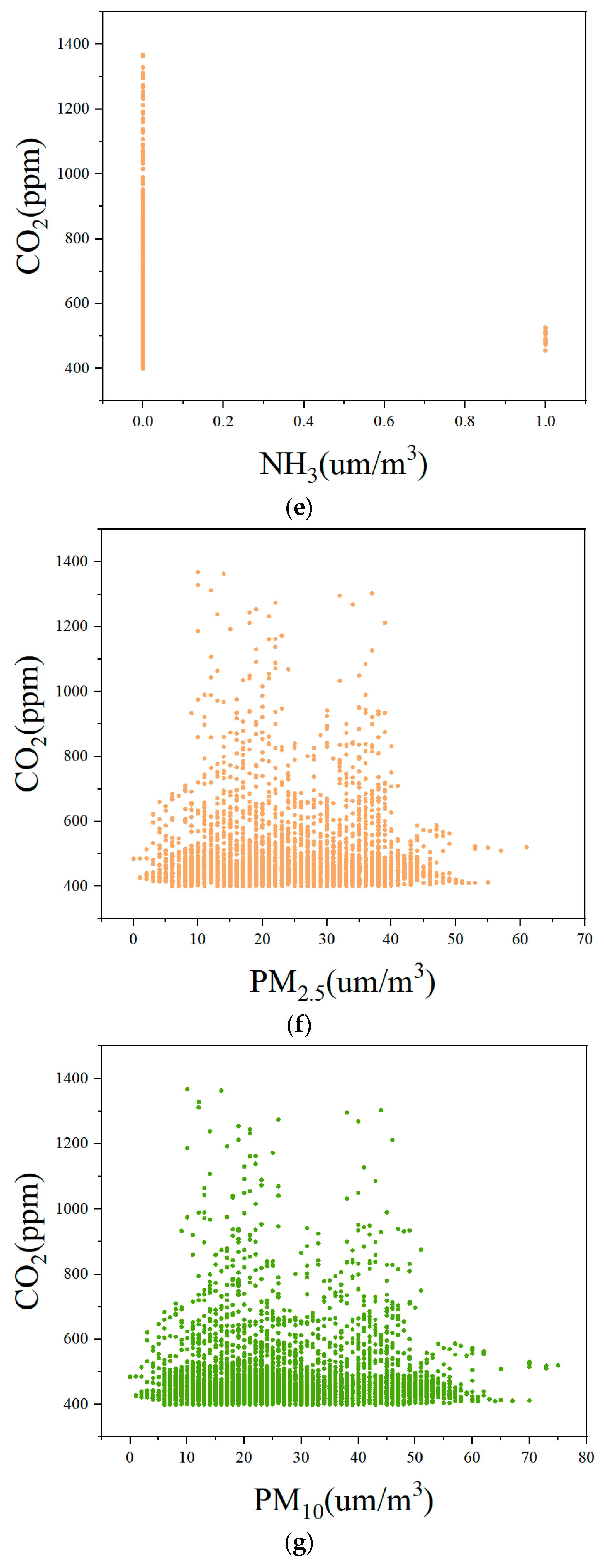
The purpose of this study was to construct a CO₂ concentration prediction model based on the screening of influencing factors affecting the CO₂ concentration in classrooms, aiming to create a comfortable and efficient classroom environment. We initially performed data preprocessing operations on the collected datasets and identified the factors influencing CO₂ concentrations using the RF algorithm. Then, we developed an RF-LSTM model using the final dataset obtained from the screening process. Following hyperparameter optimization with the Bayesian optimization algorithm, TPE, we introduced the RF-TPE-LSTM model. We then used both models to predict the indoor CO₂ concentration before and after hyperparameter optimization. The calculation results revealed that the NH₃ concentration in the classroom was not an input variable to the CO₂ prediction model. Furthermore, the prediction model exhibited excellent fit with the dataset.

In addition, we analyzed the prediction performance of the RF-TPE-LSTM model over time using four evaluation metrics, namely, the R², MAE, RMSE, and MAPE, which showed that the model has good prediction ability within a certain time range. After evaluating the RF-LSTM and RF-TPE-LSTM with different combinations of hyperparameters, it is concluded that the RF-TPE-LSTM model obtains smaller errors and better R² values when predicting the CO₂ concentration in classrooms. Specifically, compared to the RF-LSTM, the RF-TPE-LSTM model reduces the MAE from 8.27 to 2.96, the RMSE from 11.71 to 5.54, and the MAPE from 1.79% to 0.60%. This indicates that the hyperparameter optimization we used has a significant effect on improving accuracy. Subsequently, we conducted experiments using the RNN, BPNN, and Optuna–LSTM models; the results indicated that the prediction accuracies of these models improved after considering the influencing factors. Therefore, the use of the RF algorithm to filter the model inputs has some versatility for multiple algorithmic models. Notably, the R² of the RF-TPE-LSTM model exceeded 98%, indicating its strong ability to predict CO₂ concentrations in classrooms. In summary, the key findings of this study are as follows:

(1)

The model developed in this research demonstrates high accuracy in forecasting classroom CO₂ concentrations.

(2)

The predictions made by the RF-TPE-LSTM model are more robust and efficient than those made by single models or models using only one optimization algorithm.

(3)

The RF-TPE-LSTM model combines RF for feature importance analysis, TPE for hyperparameter tuning, and LSTM for time series prediction. This integration not only highlights the most significant factors influencing CO₂ levels but also fine-tunes the model’s hyperparameters, such as the number of units, learning rate, and training epochs. The collaboration of these techniques enhances the model’s capability to adapt to the dynamic variations in classroom environments, leading to better prediction accuracy and reliability.

Consequently, the model proposed in this paper can serve as an effective method for predicting CO₂ concentrations in classrooms, providing valuable data support for ventilation strategies aimed at controlling indoor CO₂ concentrations. Decision-makers responsible for controlling the physical environment of classrooms can also use our proposed CO₂ concentration prediction model to proactively utilize air-conditioning systems for ventilation, ensuring a comfortable learning environment [46,47]. Although our CO₂ concentration prediction model has achieved excellent results, we aim to address some practical issues in future work. For instance, we can develop an intuitive visualization interface to display historical CO₂ concentration data, prediction results, and model performance, making it easier for users to understand and use. This work can serve as an important component in the automatic ventilation control of CO₂ concentration in classrooms.

References

1. Klepeis, N.E.; Nelson, W.C.; Ott, W.R.; Robinson, J.P.; Tsang, A.M.; Switzer, P.; Behar, J.V.; Hern, S.C.; Engelmann, W.H. The National Human Activity Pattern Survey (NHAPS): A resource for assessing exposure to environmental pollutants. J. Expo. Sci. Environ. Epidemiol. 2001, 11, 231–252. [Google Scholar] [CrossRef] [PubMed]
2. Tang, X.M.; Wu, N.; Pan, Y. Prediction of particulate matter 2.5 concentration using a deep learning model with time-frequency domain information. Appl. Sci. 2023, 13, 12794. [Google Scholar] [CrossRef]
3. Woo, J.; Rajagopalan, P.; Andamon, M.M. An evaluation of measured indoor conditions and student performance using d2 Test of Attention. Build. Environ. 2022, 214, 108940. [Google Scholar] [CrossRef]
4. Hu, L.; Fan, N.; Li, J.; Liu, Y. Dynamic forecasting model for indoor pollutant concentration using recurrent neural network. Indoor Built Environ. 2020, 30, 1835–1845. [Google Scholar] [CrossRef]
5. Li, X.; Fang, X.; Yan, Y. In-depth investigation of air quality and CO2 lock-up phenomenon in pilots’ local environment. Exp. Comput. Multiph. Flow 2024, 6, 170–179. [Google Scholar] [CrossRef]
6. Elbayoumi, M.; Ramli, N.A.; Yusof, N.; Al Madhoun, W. Seasonal variation in schools’ indoor air environments and health symptoms among students in an eastern mediterranean climate. Hum. Ecol. Risk Assess. 2015, 21, 184–204. [Google Scholar] [CrossRef]
7. Vilén, L.; Atosuo, J.; Putus, T. The association of voice problems with exposure to indoor air contaminants in health care centres–The effect of remediation on symptom prevalence: A follow-up study. Indoor Built Environ. 2024, 33, 314–324. [Google Scholar] [CrossRef]
8. Ramalho, O.; Wyart, G.; Mandin, C.; Blondeau, P.; Cabanes, P.A.; Leclerc, N.; Mullot, J.U.; Boulanger, G.; Redaelli, M. Association of carbon dioxide with indoor air pollutants and exceedance of health guideline values. Build. Environ. 2015, 93, 115–124. [Google Scholar] [CrossRef]
9. Li, T.T.; Bai, Y.H.; Liu, Z.R.; Liu, J.F.; Zhang, G.S.; Li, J.L. Air quality in passenger cars of the ground railway transit system in Beijing, China. Sci. Total Environ. 2006, 367, 89–95. [Google Scholar] [CrossRef] [PubMed]
10. Allen, J.G.; MacNaughton, P.; Satish, U.; Santanam, S.; Vallarino, J.; Spengler, J.D. Associations of cognitive function scores with carbon dioxide, ventilation, and volatile organic compound exposures in office workers: A controlled exposure study of green and conventional office environments. Environ. Health Perspect. 2016, 124, 805–812. [Google Scholar] [CrossRef] [PubMed]
11. Zhang, X.; Wargocki, P.; Lian, Z. Physiological responses during exposure to carbon dioxide and bioeffluents at levels typically occurring indoors. Indoor Air 2017, 27, 65–77. [Google Scholar] [CrossRef] [PubMed]
12. Wargocki, P.; Porras-Salazar, J.A.; Contreras-Espinoza, S.; Bahnfleth, W. The relationships between classroom air quality and children’s performance in school. Build. Environ. 2020, 173, 106749. [Google Scholar] [CrossRef]
13. Fuoco, F.C.; Stabile, L.; Buonanno, G.; Trassiera, C.V.; Massimo, A.; Russi, A.; Mazaheri, M.; Morawska, L.; Andrade, A. Indoor air quality in naturally ventilated Italian classrooms. Atmosphere 2015, 6, 1652–1675. [Google Scholar] [CrossRef]
14. Han, J.; Lin, H.; Qin, Z.K. Prediction and comparison of in-vehicle CO2 concentration based on ARIMA and LSTM models. Appl. Sci. 2023, 13, 10858. [Google Scholar] [CrossRef]
15. Li, X.; Chen, Z.; Tu, J.; Yu, H.; Tang, Y.; Qin, C. Impact of impinging jet ventilation on thermal comfort and aerosol transmission: A numerical investigation in a densely-occupied classroom with solar effect. J. Build. Eng. 2024, 94, 109872. [Google Scholar] [CrossRef]
16. Luther, M.B.; Horan, P.; Tokede, O. Investigating CO2 concentration and occupancy in school classrooms at different stages in their life cycle. Archit. Sci. Rev. 2018, 61, 83–95. [Google Scholar] [CrossRef]
17. Teleszewski, T.; Gladyszewska-Fiedoruk, K. The concentration of carbon dioxide in conference rooms: A simplified model and experimental verification. Int. J. Environ. Sci. Technol. 2019, 16, 8031–8040. [Google Scholar] [CrossRef]
18. Yalcin, N.; Balta, D.; Ozmen, A. A modeling and simulation study about CO2 amount with web-based indoor air quality monitoring. Turk. J. Electr. Eng. Comput. Sci. 2018, 26, 1390–1402. [Google Scholar] [CrossRef]
19. Choi, J.; Roberts, D.C.; Lee, E. Forecast of CO2 emissions from the U.S. transportation sector: Estimation from a double exponential smoothing model. J. Transp. Res. Forum. 2014, 53, 63–81. [Google Scholar] [CrossRef]
20. Xiang, X.W.; Ma, X.; Ma, Z.L.; Ma, M.D. Operational carbon change in commercial buildings under the carbon neutral goal: A LASSO-WOA approach. Buildings 2022, 12, 54. [Google Scholar] [CrossRef]
21. Mardani, A.; Liao, H.C.; Nilashi, M.; Alrasheedi, M.; Cavallaro, F. A multi-stage method to predict carbon dioxide emissions using dimensionality reduction, clustering, and machine learning techniques. J. Clean. Prod. 2020, 275, 122942. [Google Scholar] [CrossRef]
22. Ahmed, M.; Shuai, C.M.; Ahmed, M. Influencing factors of carbon emissions and their trends in China and India: A machine learning method. Environ. Sci. Pollut. Res. 2022, 29, 48424–48437. [Google Scholar] [CrossRef] [PubMed]
23. Nguyen, H.D.; Tran, K.P.; Thomassey, S.; Hamad, M. Forecasting and anomaly detection approaches using LSTM and LSTM autoencoder techniques with the applications in supply chain management. Int. J. Inf. Manag. 2021, 57, 102282. [Google Scholar] [CrossRef]
24. Qader, M.R.; Khan, S.; Kamal, M.; Usman, M.; Haseeb, M. Forecasting carbon emissions due to electricity power generation in Bahrain. Environ. Sci. Pollut. Res. 2022, 29, 17346–17357. [Google Scholar] [CrossRef] [PubMed]
25. Jung, D.H.; Kim, H.S.; Jhin, C.; Kim, H.J.; Park, S.H. Time-serial analysis of deep neural network models for prediction of climatic conditions inside a greenhouse. Comput. Electron. Agric. 2020, 173, 105402. [Google Scholar] [CrossRef]
26. Sharma, P.K.; Mondal, A.; Jaiswal, S.; Saha, M.; Nandi, S.; De, T.M.; Saha, S. IndoAirSense: A framework for indoor air quality estimation and forecasting. Atmos. Pollut. Res. 2021, 12, 10–22. [Google Scholar] [CrossRef]
27. Yang, D.; Mak, C.M. Relationships between indoor environmental quality and environmental factors in university classrooms. Build. Environ. 2020, 186, 107331. [Google Scholar] [CrossRef]
28. Amayri, M.; Arora, A.; Ploix, S.; Bandhyopadyay, S.; Ngo, Q.D.; Badarla, V.R. Estimating occupancy in heterogeneous sensor environment. Energy Build. 2016, 129, 46–58. [Google Scholar] [CrossRef]
29. Genuer, R.; Poggi, J.M.; Tuleau-Malot, C. Variable selection using random forests. Pattern Recognit. Lett. 2010, 31, 2225–2236. [Google Scholar] [CrossRef]
30. Ghanbari-Adivi, F.; Mosleh, M. Text emotion detection in social networks using a novel ensemble classifier based on Parzen Tree Estimator (TPE). Neural Comput. Appl. 2019, 31, 8971–8983. [Google Scholar] [CrossRef]
31. Zhang, B.; Zhang, M.; Hong, D. Land surface temperature retrieval from Landsat 8 OLI/TIRS images based on back-propagation neural network. Indoor Built Environ. 2021, 30, 22–38. [Google Scholar] [CrossRef]
32. Choi, J.H.; Kim, D.; Ko, M.S.; Lee, D.E.; Wi, K.; Lee, H.S. Compressive strength prediction of ternary-blended concrete using deep neural network with tuned hyperparameters. J. Build. Eng. 2023, 75, 107004. [Google Scholar] [CrossRef]
33. Ismaiel, M.; Gouda, M.; Li, Y.; Chen, Y. Airtightness evaluation of Canadian dwellings and influencing factors based on measured data and predictive models. Indoor Built Environ. 2023, 32, 553–573. [Google Scholar] [CrossRef] [PubMed]
34. Emamian, S.; Lu, T.; Kruse, H.; Emamian, H. Exploring nature and predicting strength of hydrogen bonds: A correlation analysis between atoms-in-molecules descriptors, binding energies, and energy components of symmetry-adapted perturbation theory. J. Comput. Chem. 2019, 40, 2868–2881. [Google Scholar] [CrossRef] [PubMed]
35. Kirchner, K.; Zec, J.; Delibasic, B. Facilitating data preprocessing by a generic framework: A proposal for clustering. Artif. Intell. Rev. 2016, 45, 271–297. [Google Scholar] [CrossRef]
36. Nogueira, A.L.; Munita, C.S. Quantitative methods of standardization in cluster analysis: Finding groups in data. J. Radioanal. Nucl. Chem. 2020, 325, 719–724. [Google Scholar] [CrossRef]
37. AlSagri, H.; Ykhlef, M. Quantifying feature importance for detecting depression using random forest. Int. J. Adv. Comput. Sci. Appl. 2020, 11, 628–635. [Google Scholar] [CrossRef]
38. Nicodemus, K.K. Letter to the Editor: On the stability and ranking of predictors from random forest variable importance measures. Brief. Bioinform. 2011, 12, 369–373. [Google Scholar] [CrossRef]
39. Sherstinsky, A. Fundamentals of recurrent neural network (RNN) and long short-term memory (LSTM) network. Phys. D 2020, 404, 132306. [Google Scholar] [CrossRef]
40. Xue, X.H. Prediction of daily diffuse solar radiation using artificial neural networks. Int. J. Hydrogen Energy 2017, 42, 28214–28221. [Google Scholar] [CrossRef]
41. Klaar, A.C.R.; Stefenon, S.F.; Seman, L.O.; Mariani, V.C.; Coelho, L.D. Optimized EWT-Seq2Seq-LSTM with attention mechanism to insulators fault prediction. Sensors 2023, 23, 3202. [Google Scholar] [CrossRef] [PubMed]
42. Wang, B.B.; Lu, X.J.; Ren, Y.Z.; Tao, S.; Gao, W.L. Prediction model and influencing factors of CO2 micro/nanobubble release based on ARIMA-BPNN. Agriculture 2022, 12, 445. [Google Scholar] [CrossRef]
43. Yang, G.; Yuan, E.; Wu, W. Predicting the long-term CO2 concentration in classrooms based on the BO–EMD–LSTM model. Build. Environ. 2022, 224, 109568. [Google Scholar] [CrossRef]
44. Wang, X.; Fan, Y.G. Hyperspectral image classification based on modified DenseNet and spatial spectrum attention mechanism. Laser Optoelectron. Prog. 2022, 59, 12. [Google Scholar] [CrossRef]
45. Gülmez, B. Stock price prediction with optimized deep LSTM network with artificial rabbits optimization algorithm. Expert Syst. Appl. 2023, 227, 120346. [Google Scholar] [CrossRef]
46. Taheri, S.; Razban, A. Learning-based CO2 concentration prediction: Application to indoor air quality control using demand-controlled ventilation. Build. Environ. 2021, 205, 108164. [Google Scholar] [CrossRef]
47. Vignolo, A.; Gómez, A.P.; Draper, M.; Mendina, M. Quantitative assessment of natural ventilation in an elementary school classroom in the context of COVID-19 and its impact in airborne transmission. Appl. Sci. 2022, 12, 9261. [Google Scholar] [CrossRef]
Figure 1. Overall CO2 concentration prediction framework.
Applsci 14 06188 g001
Figure 2. Actual classroom view.
Applsci 14 06188 g002
Figure 3. Data collection system overview.
Applsci 14 06188 g003
Figure 4. Sensors used in this study: (a) interior structure; (b) overall appearance.
Applsci 14 06188 g004
Figure 5. RF principle process.
Applsci 14 06188 g005
Figure 6. Core structure of the LSTM model.
Applsci 14 06188 g006
Figure 7. Hyperopt workflow based on the TPE algorithm.
Applsci 14 06188 g007
Figure 8. Preprocessing of past CO2 concentration data.
Applsci 14 06188 g008
Figure 9. Scatter plot between each environmental factor and the CO2 concentration: (a) between temperature and CO2; (b) between Humidity and CO2; (c) between Illuminance and CO2; (d) between O2 and CO2; (e) between NH3 and CO2; (f) between PM2.5 and CO2; (g) between PM10 and CO2; (h) between Indoor population and CO2; (i) between CO2_pre and CO2.
Applsci 14 06188 g009aApplsci 14 06188 g009bApplsci 14 06188 g009cApplsci 14 06188 g009d
Figure 10. Loss function variation curve with the number of iterations.
Applsci 14 06188 g010
Figure 11. Fitted results of the models on the datasets: (a1) RF-LSTM model training set, (b1) RF-LSTM model test set; (a2) RF-TPE-LSTM model training set, and (b2) RF-TPE-LSTM model test set.
Applsci 14 06188 g011
Figure 12. Prediction performance of the RF-TPE-LSTM model.
Applsci 14 06188 g012