Correction Compensation and Adaptive Cost Aggregation for Deep Laparoscopic Stereo Matching

Featured Application

This work explores the computation of disparity in stereoscopic laparoscopic images through stereo matching algorithms. By integrating the focal length and baseline of the laparoscopic vision system, we can transform the disparity into depth measurements. This digitized depth information facilitates the three-dimensional reconstruction of surgical scenes, and the real-time three-dimensional reconstructed images have the potential to provide supplementary guidance information to surgeons during procedures, thereby reducing surgical risks. Additionally, by leveraging this known digitized depth information, surgical robots can synchronize their movements with beating organs, thus reducing the complexity of such surgeries.

Abstract

Perception of digitized depth is a prerequisite for enabling the intelligence of three-dimensional (3D) laparoscopic systems. In this context, stereo matching of laparoscopic stereoscopic images presents a promising solution. However, the current research in this field still faces challenges. First, the acquisition of accurate depth labels in a laparoscopic environment proves to be a difficult task. Second, errors in the correction of laparoscopic images are prevalent. Finally, laparoscopic image registration suffers from ill-posed regions such as specular highlights and textureless areas. In this paper, we make significant contributions by developing (1) a correction compensation module to overcome correction errors; (2) an adaptive cost aggregation module to improve prediction performance in ill-posed regions; (3) a novel self-supervised stereo matching framework based on these two modules. Specifically, our framework rectifies features and images based on learned pixel offsets, and performs differentiated aggregation on cost volumes based on their value. The experimental results demonstrate the effectiveness of the proposed modules. On the SCARED dataset, our model reduces the mean depth error by 12.6% compared to the baseline model and outperforms the state-of-the-art unsupervised methods and well-generalized models.

1. Introduction

Three-dimensional laparoscopic systems have demonstrated the potential to decrease the duration of minimally invasive surgery (MIS) and potentially minimize perioperative complications, especially in procedures involving laparoscopic suturing [1]. But they currently can only display stereoscopic images through polarized glasses to provide surgeons with depth perception, without the capability to calculate digital depth information. Digitalization is a prerequisite for informatization and intelligentization. Accurately digitizing depth perception poses a significant challenge in the context of intellectualized 3D laparoscopic systems. However, range-finding sensors such as LiDAR systems are not convenient for robot-assisted MIS because of the limited port size and requirements of sterilization. As an alternative, binocular stereo laparoscopes can satisfy these conditions and have the potential to address the depth perception problem by implementing stereo matching techniques [2]. For pixels in one view of a pair of stereo images, stereo matching aims to find their corresponding pixels along the epipolar lines in the other view, and to output the disparity d, namely, the horizontal displacement between a pair of corresponding pixels. Then, the depth can be calculated by $\frac{f·b}{d}$, where f is the camera’s focal length and b is the distance between two camera centers.

Stereo matching has become an active area of research in the field of computer vision. In recent years, benefiting from deep learning technology and large synthetic datasets, stereo matching for natural images such as KITTI 2015 [3] and Middlebury [4] has made substantial progress [5,6,7,8,9]. However, acquiring dense depth information from laparoscopic stereo images remains a non-trivial task. Several challenges have led to this situation. First, there is a scarcity of datasets in the surgical domain owing to limitations in acquiring accurate depth information using conventional depth sensors. Publicly available datasets with precise depth labels can hardly support supervised learning methods [2,10,11]. Second, perfect correction is difficult to obtain from stereoscopic images during surgery because of errors from camera calibration [12,13,14,15,16] and intraoperative focusing [17,18], whereas most state-of-the-art stereo networks are designed on this premise. Figure 1 shows an example of correction error, where the blue solid lines connect the matching point pairs, and the white dashed lines represent the horizontal lines. The angle between these two lines indicates the vertical correction error between the matching points. As the camera calibration is a homography transformation, correction errors also exist in the horizontal direction, although they are difficult to visualize. Third, large textureless areas in smooth tissues and organs, as well as specular highlights present challenges for registration.

The lack of labeled datasets has made researchers focus more on the self-supervised learning ability of stereo networks, which has been shown to be promising [11,20,21]. Given that [21] relies on the parallax attention mechanism, which possesses a global receptive field, and consequently, has advantages in the registration of textureless areas, in this work, we followed [21] and extended it to the application scenario of endoscopic surgery. On this basis, we designed a correction compensation module to alleviate the negative effects caused by imperfect correction of laparoscopic stereo images. To enhance prediction effectiveness in areas with specular highlights and no texture, we further developed an adaptive cost aggregation module to guide the network to make greater use of high-value cost information determined by a unimodal distribution coefficient. Simultaneously, this module leverages interleaved group convolution structure (IGCS) and dense connection structure (DCS) to ensure the preservation of the original accuracy while reducing the overall complexity of the model.

In summary, the main contributions of this paper are as follows:

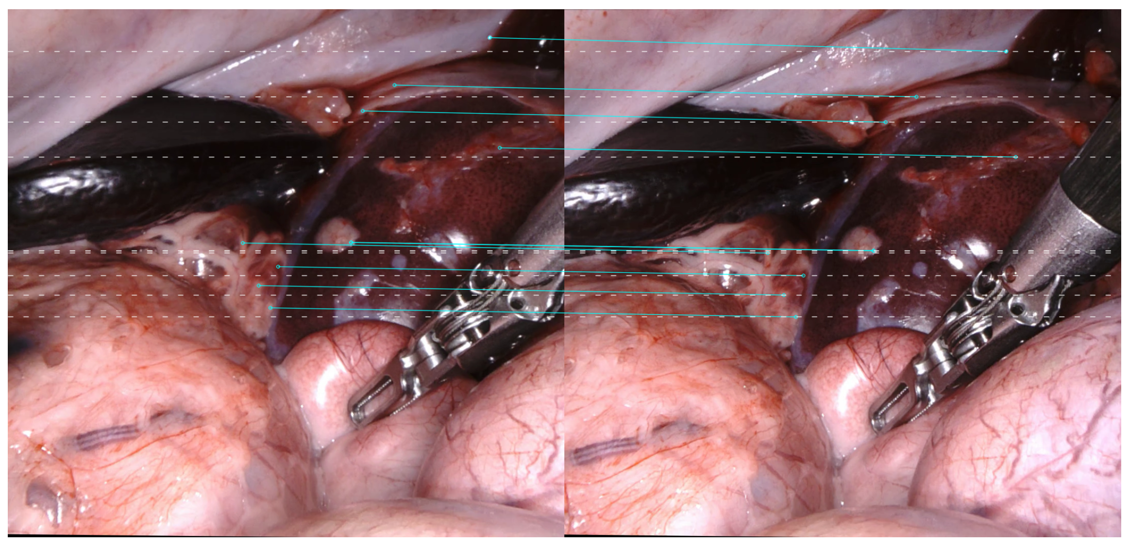
• A correction compensation module is proposed to overcome correction errors. Unlike previous work, we learn about correction error information from a real laparoscopic dataset and compensate for errors in both the horizontal and vertical directions.
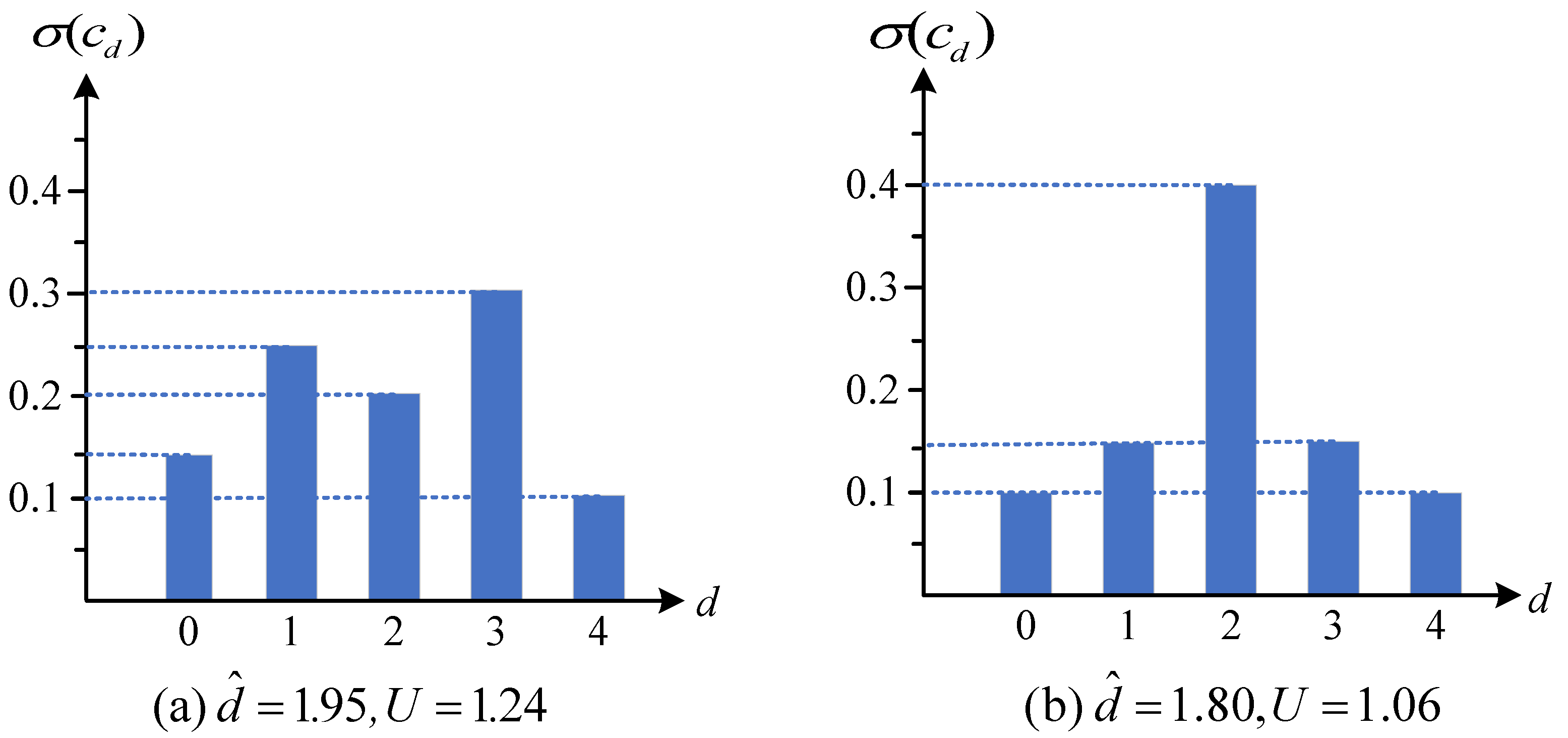
• An adaptive cost aggregation module is proposed to improve prediction performance in ill-posed regions. We skillfully quantify the value of cost volume elements based on their distribution and theoretically link high-value elements to those in ill-posed regions. By emphasizing high-value elements during the cost aggregation process, we improve the regularization effect on elements in ill-posed areas.
• Without ground truth labels, we propose an unsupervised depth estimation method for stereo laparoscopic images based on the proposed modules. Our model outperforms the state-of-the-art unsupervised methods and well-generalized models.

2. Related Work

In this section, we provide a brief overview of the research status of stereo matching algorithms, including those based on deep learning and those designed for laparoscopic images.

2.1. Learning-Based Stereo Matching

Recently, learning-based stereo matching networks have achieved state-of-the-art performance. Mayer [22] proposed the first end-to-end stereo matching network, DispNet, and its correlation version DispNetC. Kendall et al. [23] introduced a novel approach in which they formulated a cost volume by concatenating the features extracted from an image pair and subsequently aggregated it through the utilization of 3D convolutions. Subsequent work primarily builds upon these two frameworks.

For better performance in ill-posed image areas such as textureless surfaces, specular highlights, and occlusions, Chang et al. [5] proposed a pyramid stereo matching network that incorporated a spatial pyramid pooling module to expand the receptive fields and capture more representative features, which were then aggregated using stacked 3D hourglass networks. Zhang et al. [24] made traditional semi-global and local matching algorithms differentiable and applied them in the cost aggregation phase. Xu et al. [9] treated the correlation cost volume as an attention module for the concatenation cost volume, guiding the concatenation operation to retain more information useful for registration, and introduced a multi-level adaptive patch matching module to improve the distinctiveness of the matching cost at different disparities even for textureless regions. Liu et al. [25] proposed the local similarity pattern to learn the relationships among weights within a convolutional kernel, which reflects the local structural property. The authors also designed a dynamic self-reassembling refinement strategy and applied it to the cost distribution and the disparity map, respectively. This strategy allowed the elements within the cost volume and disparity map to fuse information from a limited number of neighboring elements, and enabled better information aggregation for isolated elements near occlusions.

To address the challenge of acquiring accurate depth labels in special scenarios, such as surgical environments, researchers have advocated for self-supervised stereo matching approaches. Zhou et al. [20] employed a left–right consistency check to generate confidence maps, thereby guiding the training of networks. Yang et al. [26] conducted semantic feature embedding and regularized semantic cues as the loss term to improve learning disparity. Li et al. [27] proposed a stereo matching network utilizing occlusion information, where the authors introduced an occlusion inference module to provide occlusion cues. Additionally, they proposed a hybrid loss that leverages the interaction between disparity and occlusion to guide the training process. Wang et al. [21] introduced a parallax attention mechanism (PAM) and used it to construct the self-supervised stereo matching network, PASMnet. The inherent left–right consistency and cyclic consistency of PAM acts as additional guidance for model training, and PAM efficiently calculates the feature correlation between any two positions along the epipolar line, which helps to avoid the necessity for the network to set a fixed maximum disparity.

To address the problem of correction errors present in real-world datasets, Li et al. [12] proposed an adaptive group correlation layer that allows for offsets in the feature elements participating in correlation calculations. This design avoided the exclusion of misaligned features caused by correction errors during the feature similarity computation. The adaptive group correlation layer effectively copes with stereo image pairs that are insufficiently rectified, offering a solution for the application of stereo matching algorithms on consumer-grade devices. However, the authors simulate correction errors using data augmentation techniques such as random homography transformation on synthetic datasets, which differ from real image correction errors. This discrepancy somewhat limits the model’s ability to capture true image correction errors in real scenarios.

Overall, deep learning techniques and large datasets have greatly advanced stereo matching algorithms when applied to natural images such as outdoor highway scenes. Among these algorithms, supervised ones have shown better performance and are even capable of handling challenges in registration, such as specular highlights, large textureless regions and correction errors. Relatively speaking, due to the lack of the strong supervisory signal, i.e., disparity regression loss, self-supervised models still face challenges in dealing with these difficulties.

2.2. Stereo Matching for Laparoscopic Images

With the great progress that modern deep learning systems have made on nature images, a promising next challenge is surgical stereo vision, e.g., laparoscopic images [10]. It has been widely researched as a prerequisite for downstream medical tasks such as surgical robot navigation and virtual reality. Li et al. [28] were the first to utilize a sequence-to-sequence Transformer model to address the stereo matching task. Benefiting from the global receptive field of the Transformer, the proposed STTR model demonstrated superior performance in regions with large disparity ranges and occlusions, and exhibited better generalization capabilities compared to traditional convolutional neural network (CNN) methods, achieving impressive results when directly tested on laparoscopic datasets. Cheng et al. [10] explored the performance of CNN and Transformer architectures in various components of stereo matching networks for laparoscopic images. They concluded that using Transformers for learning feature representations and CNNs for aggregating matching costs led to faster convergence, higher accuracy, and improved generalization capabilities. Concurrently, the authors introduced a stereo matching network, HybridStereo, which integrates CNN and Transformer structures. This network achieved state-of-the-art performance on laparoscopic datasets due to its generalization. Luo et al. [15] observed the significant correction errors in laparoscopic images and developed a vertical correction module to address this challenge in a self-supervised manner. However, this work ignored the correction errors along the horizontal direction. Yang et al. [17] also pointed out that camera adjustments during an intervention make it uncommon to acquire endoscopy image acquisition accompanied by accurately calibrated camera parameters. Hence, they utilized an unsupervised optical flow network to estimate depth, during which no camera parameters were required. However, the authors recovered the depth from the optical flow using the mid-point triangulation method, during which the stereo calibration parameters were still essential and errors were unavoidable.

In summary, current mainstream efforts have not explicitly captured the correction errors in laparoscopic images and compensated for alignment in both vertical and horizontal directions to overcome correction errors. Moreover, recent work has barely addressed improving the quality of disparity prediction in ill-posed areas from the perspective of value differences in cost volume elements.

3. Materials and Methods

In this section, an overview of our network is presented. Then, we introduce the details of the proposed correction compensation module and adaptive cost aggregation module.

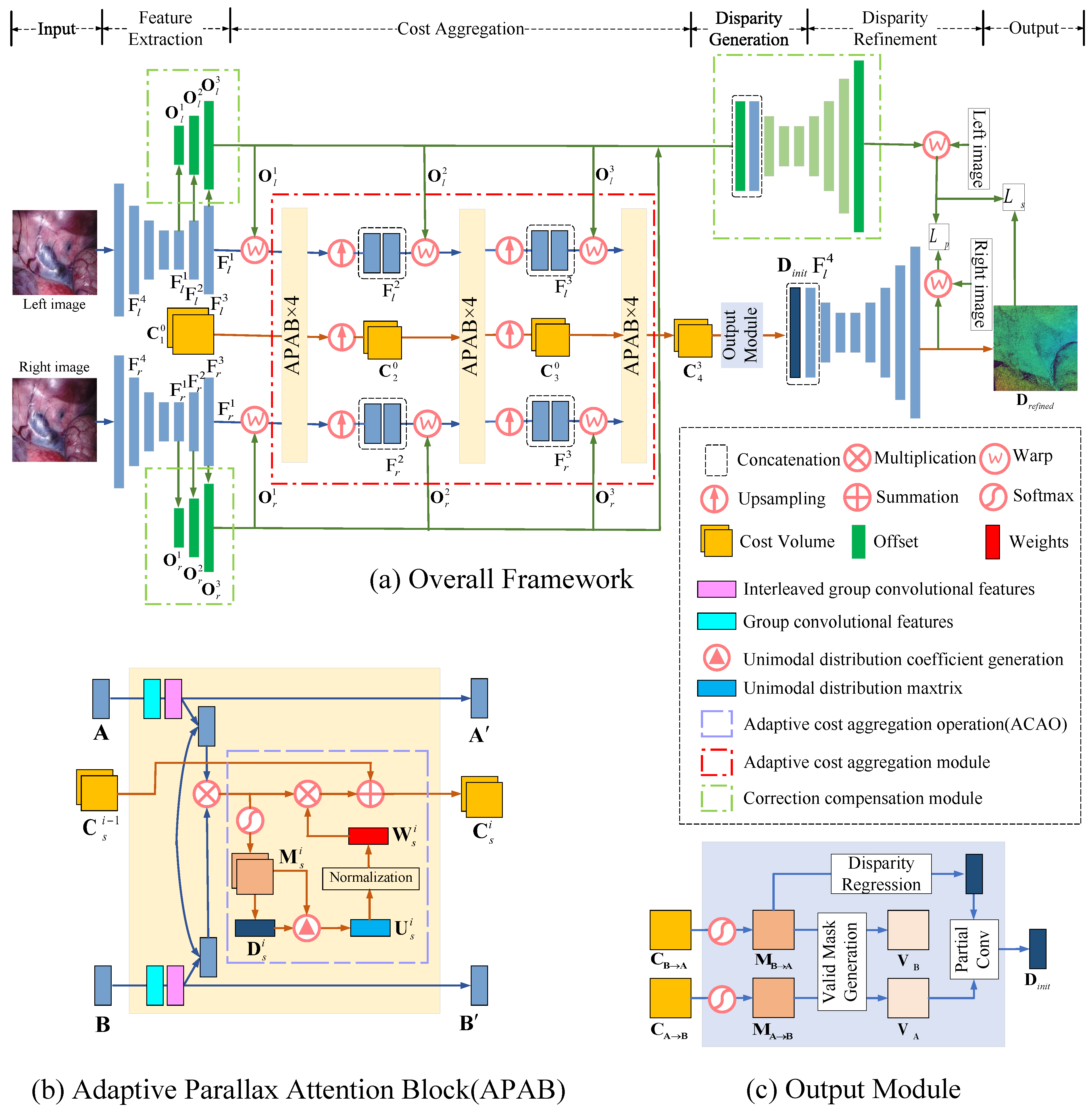
3.1. Network Architecture

Our network is depicted in Figure 2, and it consists of four steps: feature extraction, cost aggregation, disparity generation, and disparity refinement. As with our benchmark model [21], the feature extraction and disparity refinement tasks are dealt with using hourglass networks. During the disparity generation step, the aggregated costs (${\mathbf{C}}_{\mathbf{A}\to \mathbf{B}}$ and ${\mathbf{C}}_{\mathbf{B}\to \mathbf{A}}$) are successively converted into parallax attention maps (${\mathbf{M}}_{\mathbf{A}\to \mathbf{B}}$ and ${\mathbf{M}}_{\mathbf{B}\to \mathbf{A}}$) and valid masks (${\mathbf{V}}_{\mathbf{A}}$ and ${\mathbf{V}}_{\mathbf{B}}$). Then, the initial disparity ${\mathbf{D}}_{init}$ is the sum of all disparity candidates weighted by the parallax attention map. For an invalid pixel, its initial parallax is derived from a partial convolution.

In particular, aiming at alleviating the situation in which the corresponding pixels are imperfectly aligned caused by imperfect correction, our network comprises a correction compensation module. In addition, we redesigned a cost aggregation network, i.e., adaptive cost aggregation module. It consists of 12 adaptive parallax attention blocks (APABs), which capture stereo correspondence using group convolution and the proposed interleaved group convolution, and reconstruct the cost volume according to its elements’ value differences. These APABs are evenly divided into three groups for different input sizes. APABs in the same group pass information losslessly through a dense connected structure.

3.2. Correction Compensation Module

Errors in camera calibration can be represented by a homography matrix $H\in {\mathbb{R}}^{3\times 3}$ [29], resulting in a corrected practical image denoted as $I_{\mathrm{imperfect}}=I_{\mathrm{perfect}}\left(\mathcal{W}(p,Hp)\right)$, where p denotes the image coordinate and $\mathcal{W}$ represents the warp operation. It is natural to recognize that imperfect alignment includes both vertical and horizontal shifts. This was also observed by [15], but they only addressed vertical offsets. In this paper, we propose a correction compensation module to cope with both vertical and horizontal shifts caused by imperfect calibration.

Our correction compensation module consists of a feature compensation part and an image compensation part. As depicted in Figure 2, within the feature correction part, three convolution combinations are utilized to learn the offsets of features at 1/4, 1/8, and 1/16 scales, respectively. Each combination employs a 3 × 3 convolution to learn the offset information of pixels in the feature maps as well as a $1\times 1$ convolution to integrate the information into a two-channel output. In the image compensation part, we use an hourglass network to mine the offset information from the shallow feature at 1/4 scale and the feature offset map at the same scale.

To facilitate the proper learning of offsets by the correction compensation module, we introduce additional constraints to the network based on prior knowledge of correction targets. Initially, according to the general camera imaging and image correction outcomes, we do not encourage large offsets. Consequently, we impose exponential constraints on the absolute value of the offset, which can be formulated as follows:

$$L_{\mathrm{mag}}=\sum _{s\in \{1,2,3,4\}}\frac{{\lambda }_s}{N}\left({\parallel e^{|{\mathbf{O}}_l^s|}+e^{|{\mathbf{O}}_r^s|}\parallel }_1\right),$$

(1)

where $s\in \{1,2,3,4\}$ denotes 1/16, 1/8, 1/4, and full scale, respectively. ${\mathbf{O}}_l^s$ and ${\mathbf{O}}_r^s$ denote the left and right offset maps at s scale, respectively. ${\lambda }_s$ denotes the weight coefficient of the magnitude loss at s scale. N denotes the number of pixels involved in the loss calculation. Note that in the formulas, the values in the offset maps are normalized; however, the offsets are measured in pixels during the compensation process. We limit the maximum offset for features at the 1/16 scale to be m, which is a hyperparameter, and the maximum offset for features at other scales is a multiple of m, specifically determined by the ratio of their resolutions.

Moreover, to ensure consistency among offset maps of different scales, we apply a scale constraint to the absolute differences between offset maps at adjacent scales. This constraint is defined as follows:

$$L_{\mathrm{scale}}=\sum _{s\in \{1,2,3\}}\frac{{\mu }_s}{N}{\parallel {\mathbf{O}}^s-\mathtt{interp}\left({\mathbf{O}}^{s+1}\right)\parallel }_1,$$

(2)

where $s\in \{1,2,3\}$ denotes 1/16, 1/8, and 1/4 scales, respectively. ${\mathbf{O}}^s$ denotes the left or right offset map at s scale. ${\mu }_s$ denotes the weight coefficient of the scale loss at s scale. And $\mathtt{interp}$ denotes the bilinear interpolation operation, where the scale factor is 0.5 or 0.25 depending on the ratio of their resolutions.

In addition, for a pair of matching points, the offset from the left image to the right image and that from the right image to the left image should be inversely correlated. Therefore, we utilize the left–right consistency loss to constrain the absolute value of their sum, which is formulated as follows:

$$L_{\mathrm{lr}}=\sum _{s\in \{1,2,3,4\}}\frac{{\nu }_s}{N}{\parallel {\mathbf{O}}_l^s+{\mathbf{O}}_r^s\parallel }_1,$$

(3)

where ${\nu }_s$ denotes the weight coefficient of the left–right consistency loss at s scale. Finally, the loss of our correction compensation module can be expressed as

$$L_C=L_{\mathrm{mag}}+L_{\mathrm{scale}}+L_{\mathrm{lr}}.$$

(4)

3.3. Adaptive Cost Aggregation Module

As depicted in Figure 2b, the left and right feature maps of size ${\mathbb{R}}^{H\times W\times C}$ are first fed to $1\times 1$ convolutions to produce a query feature map $\mathbf{Q}\in {\mathbb{R}}^{H\times W\times C}$ and a key feature map $\mathbf{K}\in {\mathbb{R}}^{H\times W\times C}$. Then, matrix multiplication is performed between $\mathbf{Q}$ and $\mathbf{K}$ to generate the cost volume $\mathbf{C}\in {\mathbb{R}}^{H\times W\times W}$. In our baseline method [21], these cost volumes are directly summed up during the cost aggregation stage. However, this aggregation method overlooks the value differences among elements within the cost volume. Intuitively, capturing stereo consistency in ill-posed areas such as specular highlights and textureless regions of an image is more challenging than in other areas. During the cost aggregation process, a greater focus should be placed on the elements within ill-posed areas. Thus, we construct an adaptive cost aggregation module that leverages the distribution information of the cost volume to assess the value of its elements, and explicitly guide the network to strengthen the cost aggregation for elements of high value, which correspond to those within ill-posed areas. This step is referred to as the adaptive cost aggregation operation (ACAO). Furthermore, the adaptive cost aggregation module incorporates the proposed interlaced group convolution structure (IGCS) and dense connection structure (DCS). They are designed to reduce the computational complexity and parameters while preserving the accuracy of the aggregation process.

3.3.1. Adaptive Cost Aggregation Operation

Applying softmax to the cost volume $\mathbf{C}$ yields the parallax attention map $\mathbf{M}\in {\mathbb{R}}^{H\times W\times W}$. Assuming $\mathbf{Q}$ derives from the left features, and $\mathbf{K}$ derives from the right features, the point $(i,j,k)$ on $\mathbf{M}$ indicates that the disparity d between point $(i,j)$ in the left image and point $(i,k)$ in the right image equals $k-j$, and their registration confidence is $\mathbf{M}(i,j,k)$. We employ the standard deviation of the candidate parallax as a metric to quantify the degree of the unimodal distribution. For the point $(i,j)$ in the left image, its candidate disparities are the disparities between it and the set of points $\left\{\right(i,k\left)\right|k\ge j\}$ in the right image. The degree of unimodality and the standard deviation of the candidate parallax, i.e., the unimodal coefficient U, exhibit a negative correlation. As depicted in Figure 3, a higher degree of unimodal distribution indicates more accurate registration, signifying the pixel in the cost matrix is of lower value and contributes less to the optimization process. Therefore, it is imperative to attenuate the influence of low-value cost information while reinforcing the impact of high-value information. Mathematically, the unimodal distribution coefficient U is defined as follows:

$$\begin{array}{cc}\hfill U=& \sqrt{\sum _{\forall d\ge 0}{(d-\widehat{d})}^2\times \sigma \left(c_d\right)},\hfill \\ \hfill & \widehat{d}=\sum _{\forall d\ge 0}d\times \sigma \left(c_d\right),\hfill \end{array}$$

(5)

where d denotes the candidate disparity between one point on the left epipolar line and points on the corresponding right epipolar line. $\sigma (·)$ denotes the softmax operation. $c_d$ denotes the cost between two pixels of which the disparity is d. $\widehat{d}$ denotes the disparity regressed from the predicted cost matrix.

We further utilize learnable parameters $\alpha$ and $\beta$ to normalize the unimodal distribution matrix $\mathbf{U}$, resulting in the aggregation weight matrix $\mathbf{W}$ of the cost. This is formulated as

$${\mathbf{W}}_s^j={\alpha }_s{\mathbf{U}}_s^j+{\beta }_s,$$

(6)

where $s\in \{0,1,2\}$ denotes a different scale, and j denotes the number of APABs at the current scale. Finally, the aggregated cost is the weight summation of the cost matrix, which is formulated as follows:

$$\widehat{\mathbf{C}}=\sum _{s\in \{1,2,3\}}\sum _{i\in \{1,2,3,4\}}{\mathbf{C}}_s^i{\mathbf{W}}_s^i.$$

(7)

3.3.2. Interleaved Group Convolution Structure

Because the cost distribution information is explicitly incorporated into the disparity aggregation network, there is a possibility of parameter redundancy. To address this problem, we replace the standard convolution layers with group convolution layers. Meanwhile, we design an interleaved group convolution structure (IGCS) to make full use of the information learned through the network.

The IGCS, as depicted in Figure 4, incorporates two additional operations compared with the conventional group convolution structure (GCS). This includes an interleaving operation before the convolution and a rollback operation after the convolution. When the interleaved group convolution is utilized alone, there is no significant difference from the conventional group convolution. However, when used in conjunction with conventional group convolution, it facilitates information interaction between features in different groups, enabling the network to capture more correlation information in channels than pure conventional group convolution. Remarkably, the interleaving and rollback operations in interleaved group convolution do not require floating-point arithmetic. This means that the interleaved group convolution can enhance the learning ability of the network with minimal additional computational burden.

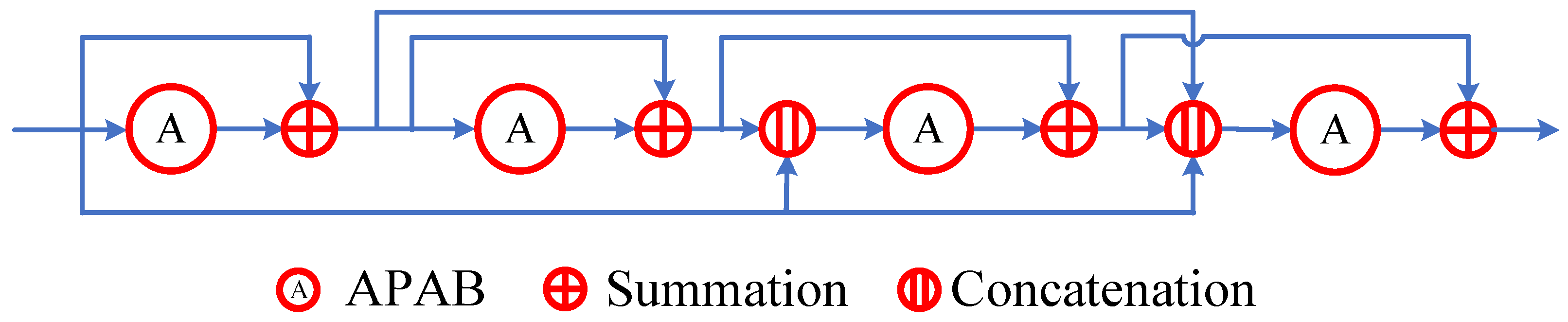
3.3.3. Dense Connection Structure

The DCS shares the same design idea as that in [30]. Specifically, at the cost aggregation stage, the feature information learned by every APAB is losslessly transmitted to subsequent modules. As shown in Figure 5, for a single APAB, its input features are transmitted to the output in an additive manner. In the case of multiple APABs, the input features of the first are transmitted to the last in a concatenated manner. The DCS is conducive to the propagation of information, strengthens the reuse of information, and avoids gradient descent, making it easier for the network to converge.

3.4. Loss

In addition to the correction loss we designed, we retained all the losses from the baseline model [21], including the photometric loss $L_{\mathrm{P}}$, disparity smoothness loss $L_{\mathrm{S}}$, and parallax attention mechanism loss $L_{\mathrm{PAM}}$. The difference lies in the computation of the photometric loss and disparity smoothness loss.

During the training process, the left and right images are alternately compensated. When compensating the left image, the input for the photometric loss consists of the compensated left image and predicted left image obtained by warping the right image. On the other hand, when compensating the right image, the input for the photometric loss consists of the left image and the predicted left image obtained by warping the compensated right image. This can be formulated as follows:

$$L_{\mathrm{P}}=\frac{1}{N}\sum _p\alpha \frac{1-\mathcal{S}(\mathbf{I}\left(p\right),\widehat{\mathbf{I}}\left(p\right))}{2}+(1-\alpha ){\parallel \mathbf{I}\left(p\right)-\widehat{\mathbf{I}}\left(p\right)\parallel }_1,$$

(8)

where $\mathbf{I}=\mathcal{W}({\mathbf{I}}_{left},{\mathbf{O}}_l)$, $\widehat{\mathbf{I}}=\mathcal{W}({\mathbf{I}}_{right},{\mathbf{D}}_{refined})$ or $\mathbf{I}={\mathbf{I}}_{left}$, $\widehat{\mathbf{I}}=\mathcal{W}(\mathcal{W}({\mathbf{I}}_{right},{\mathbf{O}}_r),{\mathbf{D}}_{refined})$, depending on which side of the image has been compensated. ${\mathbf{I}}_{left}$ and ${\mathbf{I}}_{right}$ denote the left and right input images, respectively. $\mathcal{W}$ is a warping operation and $\mathcal{S}$ is the structural similarity metric (SSIM) function. p denotes a pixel and N denotes the number of pixels. $\alpha$ is a regulatory factor, set to 0.85.

Similarly, if the left image is compensated, the input image for computing the disparity smoothness loss should be the compensated image. Otherwise, it is the original image. The smoothness loss can be formulated as follows:

$$\begin{array}{cc}\hfill L_{\mathrm{S}}=& \frac{1}{N}\sum _p({\parallel {\nabla }_x{\mathbf{D}}_{refined}\left(p\right)\parallel }_1{e}^{-{\parallel {\nabla }_x\mathbf{I}\left(p\right)\parallel }_1}+\hfill \\ & {\parallel {\nabla }_y{\mathbf{D}}_{refined}\left(p\right)\parallel }_1{e}^{-{\parallel {\nabla }_y\mathbf{I}\left(p\right)\parallel }_1}),\hfill \end{array}$$

(9)

where $\mathbf{I}={\mathbf{I}}_{left}$ or $\mathbf{I}=\mathcal{W}({\mathbf{I}}_{left},{\mathbf{O}}_l)$. ${\nabla }_x$ and ${\nabla }_y$ denote the gradients along the x and y axes, respectively.

Finally, the total loss of our network can be expressed as

$$L=L_{\mathrm{P}}+{\eta }_{\mathrm{S}}{L}_{\mathrm{S}}+{\eta }_{\mathrm{PAM}}{L}_{\mathrm{PAM}}+{\eta }_{\mathrm{C}}{L}_{\mathrm{C}}.$$

(10)

where $\eta$ is a weight coefficient.

4. Experiments and Results

In this section, we discuss the relevant experiments, including the metrics, datasets, implementation, and results.

4.1. Datasets and Metrics

We used the SCARED dataset [14] for training and testing. The SCARED dataset was released at the MICCAI Endovis Challenge and was captured using a da Vinci Xi surgical robot, Intuitive Surgical, Sunnyvale, CA, USA. It consisted of nine subsets with the content of pig enterocoelia. Each subset contained five keyframes from different perspectives, and included four to five video segments starting with these keyframes. The keyframes had accurate point cloud labels. However, labels of subsequent frames in the video were created by reprojection and interpolation of the keyframe depth maps using the kinematic information from the da Vinci robot, and consequently, had a misalignment to the RGB data. Therefore, during the ablation experiment, we utilized only the keyframes and the subsequent 19 frames of each video in the test set to calculate disparity-related metrics, including the end-point error (EPE), t-pixel error rate (Dt), and depth-related mean absolute error (MAE) for reducing the effect of cumulative errors. In the testing phase, we used the official method to evaluate the depth average error on all images in the test set. In addition, we tested our model only for keyframes and computed the structural similarity (SSIM) [31] metric for all test images. In total, we had 22,590 image pairs for training, 162 images pairs for validating, and 5907 image pairs for testing. We rectified all image pairs using OpenCV 4.6.0 and retained the boundary occlusion from the correction. For the testing set, we additionally transferred the ground truths to rectified coordinates using the provided scene points and camera parameters.

The EPE metric can be formulated as

$$\mathrm{EPE}=\frac{1}{\left|W\right|}\sum _{(x,y)\in W}|{\mathbf{D}}_{pred}(x,y)-{\mathbf{D}}_{gt}(x,y)|,$$

(11)

where W represents the set of valid pixels, where pixels with a ground truth disparity not exceeding 0 are typically excluded from the calculation; $\left|W\right|$ denotes the number of valid pixels; $D_{pred}$ represents the predicted disparity map; $(x,y)$ denotes the pixel coordinate; $D_{gt}$ represents the ground truth disparity. The t-pixel error rate can be expressed as follows:

$$\mathrm{D}t=\frac{1}{\left|W\right|}\sum _{(x,y)\in W}\left[\right|{\mathbf{D}}_{pred}(x,y)-{\mathbf{D}}_{gt}(x,y)|>\max (t,0.05\ast {\mathbf{D}}_{gt}(x,y))],$$

(12)

where t typically takes the values 1 or 3, denoted, respectively, as D1 and D3. The MAE can be expressed as follows:

$$\mathrm{MAE}=\frac{1}{\left|V\right|}\sum _{(x,y)\in V}|{\mathbf{Z}}_{pred}(x,y)-{\mathbf{Z}}_{gt}(x,y)|,$$

(13)

where V represents the set of valid pixels, where pixels with a ground truth depth not exceeding 0 are typically excluded from the calculation; $\left|V\right|$ denotes the number of valid pixels; $V_{pred}$ and $V_{gt}$ represent the predicted and the ground truth depth maps, respectively.

4.2. Implementation Details

The network was implemented using the PyTorch 1.12.0 framework with an input resolution of $256\times 512$ and a batch size of 14. An initial learning rate of $5\times {10}^{-4}$ was employed for the training process. The learning rate was halved at the third and sixth epochs to facilitate more stable and effective training. All models were optimized using the Adam optimizer with ${\beta }_1$ = 0.9 and ${\beta }_2$ = 0.999. Other hyperparameter settings are presented in

Table 1. The hyperparameter settings.

Hyperparameter	Value	Description
m	4	Maximum pixel offset for features of 1/16 scale
${\lambda }_1$	0.1	Weight coefficients for the magnitude loss $L_{\mathrm{mag}}$
${\lambda }_2$	0.1
${\lambda }_3$	0.1
${\lambda }_4$	0.5
${\mu }_1$	1	Weight coefficients for the scale loss $L_{\mathrm{scale}}$
${\mu }_2$	1
${\mu }_3$	1
${\nu }_1$	0.05	Weight coefficients for the left–right consistency loss $L_{\mathrm{lr}}$
${\nu }_2$	0.1
${\nu }_3$	0.15
${\nu }_4$	0.2
${\eta }_S$	0.1	Weight coefficients for the total loss of the network L
${\eta }_{PAM}$	1
${\eta }_C$	0.5

. All experiments were conducted using an Nvidia RTX 3090 GPU, Nvidia, Santa Clara, CA, USA.

4.3. Ablation Study

In this section, we introduce the ablation studies for the correction compensation module and the adaptive cost aggregation module. These experiments are designed to verify the effectiveness of each individual component within these modules, including proposed loss terms and network structures. Naturally, the overall effectiveness of each module is also validated.

4.3.1. Correction Compensation Module

The correction compensation module was designed to cope with the correction error of practical images caused by imprecise camera parameters and intraoperative focusing. The experimental results are presented in

Table 2. Ablation results for the correction compensation module. This module and its accompanying losses brought over 25% improvement in both EPE and MAE metrics, as well as over 39% improvement in D1 and D3 metrics.

dim	${\mathit{L}}_{\mathbf{mag}}$	${\mathit{L}}_{\mathbf{scale}}$	${\mathit{L}}_{\mathbf{lr}}$	EPE↓	D1↓	D3↓	MAE↓
				2.616	20.104	17.407	2.767
$x,y$				71.431	90.505	90.116	26.557
$x,y$	✓			2.641	20.690	17.887	2.765
$x,y$	✓	✓		2.244	14.338	11.986	2.475
$x,y$	✓	✓	✓	$\mathbf{1}.\mathbf{951}$	$\mathbf{12}.\mathbf{073}$	$\mathbf{9}.\mathbf{557}$	$\mathbf{1}.\mathbf{897}$
y	✓	✓	✓	2.163	14.879	12.271	2.142

↓ indicates that the smaller the value, the better the model performs.

. The first row of Table 2 presents the evaluation results of the baseline model. We integrated the correction compensation module on the baseline model without applying correction loss, and the corresponding evaluation results are shown in the second row of Table 2. It can be observed that various metrics exhibited significantly abnormal values, indicating that the network fails to converge. Subsequently, we progressively incorporated correction constraints into the network. The evaluation results are presented in rows 3 to 5 of Table 2, where these metrics are within the same order of magnitude as those of the baseline model. This suggests that the network reconverges effectively with the introduction of correction loss, demonstrating its pivotal role in guiding the training process. We could also find that when all three correction constraints were applied, the network’s EPE metric decreases from 2.616 to 1.951, and the MAE metric falls from 2.767 to 1.897, thereby demonstrating the effectiveness of the correction compensation module. Moreover, based on the data presented in the final two rows of Table 2, compensating solely for the correction error on the y axis, as opposed to simultaneous compensation on both the x and y axes, resulted in an increase in the EPE from 1.951 to 2.163 and in the MAE from 1.897 to 2.142. These results underscore the necessity of compensating for the correction error on the x axis as well.

4.3.2. Adaptive Cost Aggregation Module

The adaptive cost aggregation module aims to guide the network to aggregate more cost information of high value to improve the registration performance in areas with specular highlights and textureless regions. The corresponding experimental results are presented in

Table 3. Ablation results for the adaptive cost aggregation module. It reduces the parameter number by 18% and the floating-point operations number by 26%, while improving the model’s EPE and MAE metrics by over 5%, as well as the D1 and D3 metrics by over 14%. The number of floating-point operations was calculated through an input matrix of size $672\times 672\times 3$.

ACAO	IGCS	DCS	GCS	Params (G)↓	Flops (M)↓	EPE↓	D1↓	D3↓	MAE↓
				7.82	75.46	1.951	12.073	9.557	1.897
✓				7.82	75.46	1.873	10.367	8.314	1.799
✓	✓			6.22	52.83	1.877	10.767	8.540	1.904
✓	✓	✓		6.42	55.66	$\mathbf{1}.\mathbf{848}$	$\mathbf{10}.\mathbf{300}$	$\mathbf{8}.\mathbf{203}$	$\mathbf{1}.\mathbf{777}$
✓		✓	✓	6.42	55.66	1.952	12.035	9.566	1.897

. From the first two rows of Table 3, we observed that the EPE metric decreased from 1.951 to 1.877 if an ACAO was added to the network. By observing the loss curve shown in Figure 6, we could find that it accelerates the convergence of the model, suggesting that adaptively aggregating cost volumes based on the value differences of their elements is effective. Meanwhile, the second and third rows of Table 3 indicate that the DCS also contributed to a decrease in the EPE metric from 1.877 to 1.848. In particular, we found that the metrics became worse when only the IGCS was integrated into the network. This was because it brought about a decline in the number of learnable parameters. The IGCS was replaced with CGS to prove its effectiveness. Conclusive evidence supporting its efficacy was derived from the results obtained in the last two groups of experiments. In the end, the adaptive cost aggregation module reduced the number of network parameters by 18% and the number of floating-point operations by 26%. Additionally, it led to a slight improvement in the model performance.

4.4. Comparison Experiments

We compared our model with stereo matching methods reported in the MICCAI SCARED sub-challenge using the official evaluation code from [14]. The results are shown in the upper section of

Table 4. Comparison to reported methods on $\mathit{SCARED}$. The data represent the average depth errors. The top section of the table shows the performance of leading models in the MICCAI SCARED sub-challenge, all of which are supervised. The models in the middle section are also trained in a supervised manner, but they are not exposed to the $\mathit{SCARED}$ train set. They rely on excellent generalization to be directly evaluated on the $\mathit{SCARED}$ test set. The bottom section consists of self-supervised models. Our model achieved a fourth place performance and was in close proximity to that of the top-ranked supervised model. And our model surpassed the well-generalized models and self-supervised ones. The results of STTR and HybridStereoNet were reported in [10].

Method	Test Set I					Test Set II					Avg. (mm)
	kf1	kf2	kf3	kf4	kf5	kf1	kf2	kf3	kf4	kf5
W. Xia [14]	5.70	7.18	6.98	8.66	5.13	13.8	6.85	13.1	5.70	7.73	8.08
T. Zeffiro [14]	7.91	2.97	1.71	2.52	2.91	5.39	1.67	4.34	3.18	2.79	3.54
C. Wang [14]	6.30	2.15	3.41	3.86	4.80	6.57	2.56	6.72	4.34	1.19	4.19
J.C. Rosenthal [14]	8.25	3.36	2.21	2.03	1.33	8.26	2.29	7.04	2.22	0.42	3.74
D.P.1 [14]	7.73	2.07	1.94	2.63	0.62	4.85	0.65	1.62	0.77	0.41	2.33
D.P.2 [14]	7.41	2.03	1.92	2.75	0.65	4.78	1.19	3.34	1.82	0.36	2.63
S. Schmid [14]	7.61	2.41	1.84	2.48	0.99	4.33	1.10	3.65	1.69	0.48	2.66
STTR [28]	9.24	4.42	2.67	2.03	2.36	7.42	7.40	3.95	7.83	2.93	5.03
HybridStereoNet [10]	7.96	2.31	2.23	3.03	1.01	4.57	1.39	3.06	2.21	0.52	2.83
H. Luo [15]	8.62	2.69	2.36	2.29	2.51	6.06	0.95	2.97	0.86	1.23	3.05
PASMnet [21]	8.99	2.53	1.93	2.93	1.31	5.11	1.52	3.71	2.04	0.83	3.09
Ours	8.80	2.55	1.65	2.21	1.11	4.23	1.13	3.06	1.61	0.62	2.70

The data are measured in millimeters.

, where the data represent the average errors of the estimated depth. We only listed the top-ranked works, all of which were trained in a supervised manner. Our model achieved a fourth place performance and was in close proximity to that of the top-ranked model. Furthermore, we conducted comparisons between our model and several state-of-the-art models that were well-generalized or unsupervised. The results are presented in the middle and lower sections of Table 4, respectively. The authors of these models also noted the scarcity of labeled laparoscopic datasets. However, our solution surpassed theirs in terms of quantitative performance, as evidenced by the evaluation results.

Considering the labels of subsequent frames in the test videos were inaccurate except for the first frame, we evaluated our model only on keyframes. The left and right 100 pixels were cropped due to invalidity after correction, and pixels with a labeled disparity over 192 were excluded. The results are shown in

Table 5. Quantitative results on keyframes. Our model outperforms the baseline model by over 23% in all metrics, especially in the t-pixel error rate, where the improvement exceeds 100%. Additionally, our model demonstrates advantages over HybridStereoNet in all metrics.

Method	EPE↓	D1↓	D3↓	MAE↓
HybridStereoNet [10]	1.569	6.273	4.750	1.438
PASMnet [21]	2.279	14.640	12.779	2.242
Ours	$\mathbf{1}.\mathbf{515}$	$\mathbf{5}.\mathbf{834}$	$\mathbf{4}.\mathbf{401}$	$\mathbf{1}.\mathbf{370}$

; our model shows an improvement compared with HybridStereoNet, which achieved state-of-the-art performance in generalization ability. Our model also surpasses the benchmark PASMnet, which is a state-of-the-art unsupervised method for autonomous driving data.

Furthermore, in order to enhance the statistical significance of the evaluation results and simultaneously mitigate the interference from inaccurate labels, we computed the SSIM metric on the original left images and reconstructed left images across all images in the $\mathit{SCARED}$ test set. The results are presented in

Table 6. Evaluation results of the SSIM metric for all test images. Our model shows an improvement over the baseline model and HybridStereoNet.

Method	SSIM ↑
HybridStereoNet [10]	62.38
PASMnet [21]	62.22
Ours	$\mathbf{67}.\mathbf{20}$

and reflect the superiority of our model.

The subjective results for $\mathit{SCARED}$ are depicted in Figure 7, and the areas with noticeable differences are marked with dashed lines. In contrast to PASMnet, our model demonstrated smoother predictions that closely approximated the true values, particularly in untextured regions. For example, in the first row of Figure 7, within the surgical tool area, our predicted disparity map exhibits fewer sudden color changes, resulting in a smoother appearance that is more in line with reality. Meanwhile, in specular highlight areas, such as the dashed-line section in the second row of Figure 7, our predictions avoid significant errors.

5. Discussion

Table 4 presents the comparative results of our model with other models, categorized into three types, supervised, generalized, and self-supervised models, which are, respectively, positioned at the top, middle, and bottom parts of the table. Unlike the generalized and self-supervised models, supervised models overlook the inaccuracy of point cloud labels in the SCARED dataset, which is a theoretical flaw. Within the generalized and self-supervised categories, only our model and method [15] recognize the problem of imperfect image correction, resulting in misalignment of matching points in both the horizontal and vertical directions. Method [15] has designed a vertical correction module to address pixel shifts in the vertical direction, while our correction compensation module is designed to adjust errors in both the vertical and horizontal directions. Theoretically, image correction is a homography transformation process. Thus, compensating errors simultaneously in both directions can effectively counteract the correction inaccuracies, allowing the network backbone to focus on the registration task and thereby achieving better predictive results. Additionally, only our model performs differentiated cost aggregation based on the values of cost volume elements. This trick is used considering that the cost volume is a collection of image features, with ill-posed characteristics such as specular highlights and textureless areas scattered throughout. The registration of elements in ill-posed areas is typically more challenging compared to other elements. By emphasizing their cost information during the aggregation process, we can improve the prediction accuracy of the model.

We have demonstrated the effectiveness of the correction compensation module and the adaptive cost aggregation module through ablation studies (see Table 2 and Table 3). Thanks to these modules, our model’s predictions exhibit less noise in ill-posed areas, and are overall smoother and closer to the true values. The quantitative results in Table 4, Table 5 and Table 6 also confirm the efficacy of our proposed model, significantly enhancing the performance of the baseline model under imperfectly corrected stereo images.

It is noteworthy that our model closely matches the performance of supervised models, with the significant advantage of not relying on labels during the training process. Collecting depth labels in laparoscopic surgery scenarios is a challenging task, and the training of supervised models is hindered. Our model offers an alternative solution. Furthermore, our designed ACAO can be conveniently ported to other models. Its input and output are both three-dimensional cost volumes. Therefore, it can be directly added after the cost aggregation unit. For networks aggregating three-dimensional cost volumes, no additional operations are needed. For networks aggregating four-dimensional cost volumes, only the dimensionality of the cost volume needs to be reduced beforehand through averaging or other operations. Therefore, the work presented in this paper holds the potential to improve the performance of stereo matching in other scenarios, such as autonomous driving.

However, the disparity predictions of our model still exhibit progressive and blurry artifacts at the edges of the structures. Furthermore, under the experimental conditions described in this paper, the inference speed of the model does not yet meet the requirements for real-time performance. Our future research plan will focus on addressing these problems.

6. Conclusions

In this study, we introduced two essential modules: the correction compensation module and the adaptive cost aggregation module. The former learns and compensates for image correction errors, while the latter performs differentiated aggregation of costs based on the values of cost volume elements. Building on these modules, we proposed a reconstructed self-supervised stereo matching model. It surpasses state-of-the-art unsupervised methods and well-generalized methods, and demonstrates competitive performance compared to supervised models on the SCARED dataset. The visualization results show that our model avoids significant errors and noise more effectively than the baseline model. It achieves smoother disparities in textureless regions and reduces errors in areas with specular highlights. Our model exhibits robust capabilities in overcoming correction errors and addressing ill-posed features in images.

References

1. Arezzo, A.; Vettoretto, N.; Francis, N.K.; Bonino, M.A.; Curtis, N.J.; Amparore, D.; Arolfo, S.; Barberio, M.; Boni, L.; Brodie, R.; et al. The use of 3D laparoscopic imaging systems in surgery: EAES consensus development conference 2018. Surg. Endosc. 2019, 33, 3251–3274. [Google Scholar] [CrossRef] [PubMed]
2. Xia, W.; Chen, E.C.S.; Pautler, S.; Peters, T.M. A Robust Edge-Preserving Stereo Matching Method for Laparoscopic Images. IEEE Trans. Med. Imaging 2022, 41, 1651–1664. [Google Scholar] [CrossRef] [PubMed]
3. Menze, M.; Geiger, A. Object scene flow for autonomous vehicles. In Proceedings of the 2015 IEEE Conference on Computer Vision and Pattern Recognition (CVPR), Boston, MA, USA, 7–12 June 2015; pp. 3061–3070. [Google Scholar] [CrossRef]
4. Scharstein, D.; Hirschmüller, H.; Kitajima, Y.; Krathwohl, G.; Nešić, N.; Wang, X.; Westling, P. High-resolution stereo datasets with subpixel-accurate ground truth. Lect. Notes Comput. Sci. 2014, 8753, 31–42. [Google Scholar] [CrossRef]
5. Chang, J.R.; Chen, Y.S. Pyramid Stereo Matching Network. In Proceedings of the 2018 IEEE/CVF Conference on Computer Vision and Pattern Recognition, Salt Lake City, UT, USA, 18–23 June 2018; pp. 5410–5418. [Google Scholar] [CrossRef]
6. Xu, H.; Zhang, J. AANet: Adaptive Aggregation Network for Efficient Stereo Matching. In Proceedings of the 2020 IEEE/CVF Conference on Computer Vision and Pattern Recognition (CVPR), Seattle, WA, USA, 13–19 June 2020; pp. 1956–1965. [Google Scholar] [CrossRef]
7. Cheng, X.; Zhong, Y.; Harandi, M.; Dai, Y.; Chang, X.; Li, H.; Drummond, T.; Ge, Z. Hierarchical Neural Architecture Search for Deep Stereo Matching. In Proceedings of the Advances in Neural Information Processing Systems, Online, 6–12 December 2020; Volume 33, pp. 22158–22169. [Google Scholar]
8. Tankovich, V.; Häne, C.; Zhang, Y.; Kowdle, A.; Fanello, S.; Bouaziz, S. HITNet: Hierarchical Iterative Tile Refinement Network for Real-time Stereo Matching. In Proceedings of the 2021 IEEE/CVF Conference on Computer Vision and Pattern Recognition (CVPR), Nashville, TN, USA, 20–25 June 2021; pp. 14357–14367. [Google Scholar] [CrossRef]
9. Xu, G.; Cheng, J.; Guo, P.; Yang, X. Attention Concatenation Volume for Accurate and Efficient Stereo Matching. In Proceedings of the 2022 IEEE/CVF Conference on Computer Vision and Pattern Recognition (CVPR), New Orleans, LA, USA, 18–24 June 2022; pp. 12971–12980. [Google Scholar] [CrossRef]
10. Cheng, X.; Zhong, Y.; Harandi, M.; Drummond, T.; Wang, Z.; Ge, Z. Deep Laparoscopic Stereo Matching with Transformers. In Proceedings of the Medical Image Computing and Computer Assisted Intervention–MICCAI 2022, Singapore, 18–22 September 2022; pp. 464–474. [Google Scholar] [CrossRef]
11. Huang, B.; Zheng, J.Q.; Nguyen, A.; Xu, C.; Gkouzionis, I.; Vyas, K.; Tuch, D.; Giannarou, S.; Elson, D.S. Self-supervised Depth Estimation in Laparoscopic Image Using 3D Geometric Consistency. In Proceedings of the Medical Image Computing and Computer Assisted Intervention–MICCAI 2022, Singapore, 18–22 September 2022; pp. 13–22. [Google Scholar] [CrossRef]
12. Li, J.; Wang, P.; Xiong, P.; Cai, T.; Yan, Z.; Yang, L.; Liu, J.; Fan, H.; Liu, S. Practical Stereo Matching via Cascaded Recurrent Network with Adaptive Correlation. In Proceedings of the 2022 IEEE/CVF Conference on Computer Vision and Pattern Recognition (CVPR), New Orleans, LA, USA, 18–24 June 2022; pp. 16242–16251. [Google Scholar] [CrossRef]
13. Zhang, Z. A flexible new technique for camera calibration. IEEE Trans. Pattern Anal. Mach. Intell. 2000, 22, 1330–1334. [Google Scholar] [CrossRef]
14. Allan, M.; Mcleod, J.; Wang, C.; Rosenthal, J.C.; Hu, Z.; Gard, N.; Eisert, P.; Fu, K.X.; Zeffiro, T.; Xia, W.; et al. Stereo correspondence and reconstruction of endoscopic data challenge. arXiv 2021, arXiv:2101.01133. [Google Scholar]
15. Luo, H.; Wang, C.; Duan, X.; Liu, H.; Wang, P.; Hu, Q.; Jia, F. Unsupervised learning of depth estimation from imperfect rectified stereo laparoscopic images. Comput. Biol. Med. 2022, 140, 105–109. [Google Scholar] [CrossRef] [PubMed]
16. Hao, W.; Zhu, C.; Meurer, M. Camera Calibration Error Modeling and Its Impact on Visual Positioning. In Proceedings of the 2023 IEEE/ION Position, Location and Navigation Symposium (PLANS), Monterey, CA, USA, 24–27 April 2023; pp. 1394–1399. [Google Scholar] [CrossRef]
17. Yang, Z.; Simon, R.; Li, Y.; Linte, C.A. Dense Depth Estimation from Stereo Endoscopy Videos Using Unsupervised Optical Flow Methods. In Proceedings of the Medical Image Understanding and Analysis, Oxford, UK, 12–14 July 2021; pp. 337–349. [Google Scholar]
18. Pratt, P.; Bergeles, C.; Darzi, A.; Yang, G.Z. Practical Intraoperative Stereo Camera Calibration. In Proceedings of the Medical Image Computing and Computer-Assisted Intervention–MICCAI 2014, Boston, MA, USA, 14–18 September 2014; Golland, P., Hata, N., Barillot, C., Hornegger, J., Howe, R., Eds.; Springer: Berlin/Heidelberg, Germany, 2014; pp. 667–675. [Google Scholar]
19. Lowe, D.G. Distinctive Image Features from Scale-Invariant Keypoints. In International Journal of Computer Vision; Springer: Berlin/Heidelberg, Germany, 2004; Volume 60, pp. 91–110. [Google Scholar] [CrossRef]
20. Zhou, C.; Zhang, H.; Shen, X.; Jia, J. Unsupervised Learning of Stereo Matching. In Proceedings of the 2017 IEEE International Conference on Computer Vision (ICCV), Venice, Italy, 22–29 October 2017; pp. 1576–1584. [Google Scholar] [CrossRef]
21. Wang, L.; Guo, Y.; Wang, Y.; Liang, Z.; Lin, Z.; Yang, J.; An, W. Parallax Attention for Unsupervised Stereo Correspondence Learning. IEEE Trans. Pattern Anal. Mach. Intell. 2022, 44, 2108–2125. [Google Scholar] [CrossRef] [PubMed]
22. Mayer, N.; Ilg, E.; Häusser, P.; Fischer, P.; Cremers, D.; Dosovitskiy, A.; Brox, T. A Large Dataset to Train Convolutional Networks for Disparity, Optical Flow, and Scene Flow Estimation. In Proceedings of the 2016 IEEE Conference on Computer Vision and Pattern Recognition (CVPR), Las Vegas, NV, USA, 27–30 June 2016; pp. 4040–4048. [Google Scholar] [CrossRef]
23. Kendall, A.; Martirosyan, H.; Dasgupta, S.; Henry, P.; Kennedy, R.; Bachrach, A.; Bry, A. End-to-End Learning of Geometry and Context for Deep Stereo Regression. In Proceedings of the 2017 IEEE International Conference on Computer Vision (ICCV), Venice, Italy, 22–29 October 2017; pp. 66–75. [Google Scholar] [CrossRef]
24. Zhang, F.; Prisacariu, V.; Yang, R.; Torr, P.H. GA-Net: Guided Aggregation Net for End-To-End Stereo Matching. In Proceedings of the 2019 IEEE/CVF Conference on Computer Vision and Pattern Recognition (CVPR), Long Beach, CA, USA, 15–20 June 2019; pp. 185–194. [Google Scholar] [CrossRef]
25. Liu, B.; Yu, H.; Long, Y. Local Similarity Pattern and Cost Self-Reassembling for Deep Stereo Matching Networks. In Proceedings of the The Thirty-Sixth AAAI Conference on Artificial Intelligence, Vancouver, BC, Canada, 20–27 February 2022; Volume 36, pp. 1647–1655. [Google Scholar] [CrossRef]
26. Yang, G.; Zhao, H.; Shi, J.; Deng, Z.; Jia, J. SegStereo: Exploiting Semantic Information for Disparity Estimation. In Proceedings of the Computer Vision–ECCV 2018, Munich, Germany, 8–14 September 2018; pp. 660–676. [Google Scholar] [CrossRef]
27. Li, A.; Yuan, Z.; Ling, Y.; Chi, W.; Zhang, S.; Zhang, C. Unsupervised Occlusion-Aware Stereo Matching With Directed Disparity Smoothing. IEEE Trans. Intell. Transp. Syst. 2022, 23, 7457–7468. [Google Scholar] [CrossRef]
28. Li, Z.; Liu, X.; Drenkow, N.; Ding, A.; Creighton, F.X.; Taylor, R.H.; Unberath, M. Revisiting Stereo Depth Estimation From a Sequence-to-Sequence Perspective with Transformers. In Proceedings of the 2021 IEEE/CVF International Conference on Computer Vision (ICCV), Montreal, BC, Canada, 11–17 October 2021; pp. 6177–6186. [Google Scholar] [CrossRef]
29. Yang, G.; Manela, J.; Happold, M.; Ramanan, D. Hierarchical Deep Stereo Matching on High-Resolution Images. In Proceedings of the 2019 IEEE/CVF Conference on Computer Vision and Pattern Recognition (CVPR), Long Beach, CA, USA, 15–20 June 2019; pp. 5510–5519. [Google Scholar] [CrossRef]
30. Huang, G.; Liu, Z.; Van Der Maaten, L.; Weinberger, K.Q. Densely Connected Convolutional Networks. In Proceedings of the 2017 IEEE Conference on Computer Vision and Pattern Recognition (CVPR), Honolulu, HI, USA, 21–26 July 2017; pp. 2261–2269. [Google Scholar] [CrossRef]
31. Wang, Z.; Bovik, A.; Sheikh, H.; Simoncelli, E. Image quality assessment: From error visibility to structural similarity. IEEE Trans. Image Process. 2004, 13, 600–612. [Google Scholar] [CrossRef] [PubMed]
Figure 1. A schematic diagramof vertical calibration errors. The blue solid lines connect the matching point pairs, and the white dashed lines represent the horizontal lines. These blue key points were detected by SIFT [19] and matched using brute-force method. The angle between these two lines indicates the vertical correction error between the matching points.
Applsci 14 06176 g001
Figure 2. The overview of our network. The green box areas represents the proposed correction compensation module and the red box area represents the proposed adaptive cost aggregation module. In the training stage, the network’s photometric loss L P and disparity smoothness loss L S take the compensated images as input.
Applsci 14 06176 g002
Figure 3. An illustration of the relationship between the disparity distribution and the unimodal distribution coefficient U. In comparison, the distribution in (a) exhibits a multimodal state with a lower degree of unimodality and a larger value of U. Conversely, the distribution in (b) is unimodal, characterized by a higher degree of unimodality and a smaller value of U. That is, the lower the degree of unimodal distribution, the higher the value of U. This indicates more inaccurate registration and the corresponding cost information ought to be strengthened during the aggregation process. In this figure, d represents the candidate disparity, d ^ denotes the predicted disparity, c represents the cost, and σ is a softmax operation.
Applsci 14 06176 g003
Figure 4. An illustration of the IGCS. Interleaved group convolution, compared to conventional group convolution, introduces two additional stages: feature interleaving and feature rollback. These stages are located before and after the conventional group convolution, respectively.
Applsci 14 06176 g004
Figure 5. An illustration of the DCS. All features learned by APABs are propagated to subsequent modules using either concatenation or summation.
Applsci 14 06176 g005
Figure 6. An illustration of the descending curves of (a) the total loss and the (b) PAM loss during the training process. The PAM loss highly depends on the aggregated cost information. However, with the inclusion of ACAO, both curves exhibit a faster decline. We can infer that this operation facilitates the network in capturing high-value information from the cost matrix while filtering out low-value information, thereby accelerating the convergence of the model.
Applsci 14 06176 g006
Figure 7. Subjective results on SCARED . The areas with noticeable differences are marked with dashed lines. Compared to PASMnet, our predictions are closer to the labels. Specifically, our predictions are smoother in textureless regions and avoid significant errors in specular highlight areas.
Applsci 14 06176 g007