A Hybrid Model of Conformer and LSTM for Ocean Wave Height Prediction

Abstract

This study proposes a hybrid model (Conformer-LSTM) based on Conformer and Long Short-Term Memory networks (LSTM) to overcome the limitations of existing techniques and enhance the accuracy and generalizability of wave height predictions. The model combines the advantages of self-attention mechanisms and convolutional neural networks. It captures global dependencies through multi-head self-attention and utilizes convolutional layers to extract local features, thereby enhancing the model’s adaptability to dynamic changes in time series. The LSTM component handles long-term dependencies, optimizing the coherence and stability of predictions. Additionally, an adaptive feature fusion weight network is introduced to further improve the model’s recognition and utilization efficiency of key features. Experimental data come from the National Oceanic and Atmospheric Administration buoy data, covering wave height, wind speed, and other data from key maritime areas. Evaluation metrics include Mean Absolute Error (MAE), Root Mean Square Error (RMSE), Mean Absolute Percentage Error (MAPE), and Coefficient of Determination (R²), ensuring a comprehensive assessment of model performance. The results show that the Conformer-LSTM model outperforms traditional LSTM, CNN, and CNN-LSTM models at multiple sites, confirming its potential in wave height prediction.

1. Introduction

As global climate change and maritime activities intensify, wave height prediction has emerged as a critical research topic in marine science and ocean engineering. Accurate wave height prediction is essential for ensuring navigational safety, effective coastal planning and management, and the safety of offshore operations. However, predicting wave height is a complex and challenging task due to the dynamic nature of waves, which are influenced by various factors, including wind, tides, currents, and topography.

Time series forecasting can be categorized into one-step and multi-step prediction. While the underlying models used for both types of prediction are often similar, the key difference lies in the prediction horizon. One-step prediction, also known as single-step forecasting, involves predicting the next time point using the current and past data. In contrast, multi-step prediction forecasts several future time points, which can introduce compounding errors as predictions are made recursively or using direct multi-step strategies. This distinction is crucial in various forecasting scenarios, as the challenges and strategies for each type can differ significantly [1,2].

Accurate short-term wave height prediction can provide important information for ship navigation, helping the crew take appropriate measures to avoid the risks brought by high waves, especially under adverse weather conditions that can severely affect the safety of ships and personnel. Significant wave height prediction is crucial for improving the efficiency of marine operations and the safety of offshore and ocean-going navigation [3]. In one-step prediction of time series, data often exhibit strong nonlinearity and non-stationarity, increasing the complexity of establishing an accurate forecasting model. Nonlinearity means that data relationships cannot be captured by simple linear models, and non-stationarity means that the statistical properties of data change over time. In addition, the impact weight of multi-dimensional features on the prediction target is also very important, and data are easily affected by sudden events, introducing outliers or mutations. Addressing these anomalies and adapting the model to dynamic changes are important issues for accurate one-step prediction [4].

Current one-step prediction methods mainly include numerical simulation, statistical analysis, and deep-learning techniques.

Numerical simulation methods simulate the dynamics of waves through global and regional wave models. These models are based on physical equations and consider the impact of wind fields, currents, and atmospheric pressure to simulate wave generation, propagation, and decay. Global wave models, such as WAVEWATCH III (WW3), provide large-scale wave forecasts [5], while regional wave models, such as SWAN (Simulating Waves Nearshore) [6], offer higher resolution forecasts for specific maritime areas. Smith et al. [7] have evaluated the performance of different source term packages in WW3 wave models under various wave conditions in the Indian Ocean. Wu W, Li P, Zhai F, et al. [8] have used the SWAN wave model in the Bohai Sea, Yellow Sea, and East China Sea, evaluating the performance of seven wind resources in simulating wave height. These methods are more accurate in predicting large-scale fluctuations but have high computational costs and a high dependency on the quality and real-time updates of input data.

Statistical methods predict wave heights by analyzing the relationship between historical meteorological and wave data. By establishing regression models or using time series analysis techniques, such as the ARIMA (Autoregressive Integrated Moving Average model) [9] and SARIMA (Seasonal Autoregressive Integrated Moving Average) [2] models, statistical methods can effectively predict wave variations. Yang S, Zhang Z, Fan L, et al. [10], using the SARIMA method, have found that there is a rich wave energy resource in the waters around the Taiwan Strait, the Luzon Strait, and the northern South China Sea, with a significant increasing trend. The advantages of these methods lie in their high computational efficiency, but they may be limited by the availability and quality of historical data.

In recent years, the development of deep-learning technology has provided new ideas for solving the problem of wave height prediction [11]. Fan S, Xiao N, and Dong S. [12] proposed a model based on nearshore simulated waves and Long Short-Term Memory networks (SWAN-LSTM) for single-point prediction, which performed better than traditional statistical methods. A hybrid model combining Variational Mode Decomposition (VMD) [13] and one-dimensional Convolutional Neural Networks (CNNs) was proposed for non-stationary wave forecasting, outperforming the one-dimensional CNN. A CNN+LSTM network model [14] was used for prediction, outperforming traditional LSTM and random forest algorithms. Modal decomposition [15] was used to decompose wave height data, followed by LSTM model prediction to improve wave height prediction accuracy. Conformer, introduced by Gulati et al. in 2020 [16], with its unique structure, can effectively capture long-distance dependencies and local features in time series data by combining self-attention mechanisms and convolutional neural networks, understanding non-linear characteristics of the data. The embedded convolutional layer can extract local features, enhancing the model’s adaptability to non-stationary time series, while LSTM [17] is adept at handling time dynamics in sequence data, remembering long-term information through its gating mechanism while forgetting unimportant information, thus maintaining robustness in the face of sudden events.

This study combines the self-attention mechanism of Conformer and the Long Short-Term Memory network (LSTM) into a hybrid model, showing great potential in processing complex time series forecasting tasks. The adaptive feature fusion weight network, by dynamically adjusting the contribution of different features in the model, helps reduce unnecessary feature dimensions and focuses the learning ability of the model on the most informative features. This combination takes advantage of both models to overcome the limitations of existing methods in dealing with nonlinear and non-stationary data, providing a more accurate and stable solution for wave height prediction.

This paper is structured as follows.

Section 2 reviews the related work in the field of wave height prediction and highlights the limitations of existing models.

Section 3 details the methodology, including data collection, preprocessing steps, and the Conformer-LSTM model architecture.

Section 4 presents the experimental results, comparing the performance of the proposed model with traditional methods, and discusses the implications of the findings, potential applications, and limitations of this study.

2. Materials and Methods

This study employed a comprehensive methodology to develop and evaluate a hybrid model of Conformer and LSTM for ocean wave height prediction. The Conformer architecture, characterized by its combination of self-attention mechanisms and convolutional neural networks, was detailed. Convolutional Neural Networks (CNNs) were utilized to capture local features, while Long Short-Term Memory (LSTM) networks addressed long-term dependencies in time series data. To ensure the selection of the most relevant features, Spearman correlation analysis was conducted. The overall algorithm was designed by integrating Conformer and LSTM, followed by detailed steps involved in training the hybrid model. The algorithm process was systematically outlined, including a step-by-step guide to its implementation. The dataset, sourced from NOAA buoys, was meticulously preprocessed to handle missing and abnormal data. The performance of the model was evaluated using metrics such as MAE, RMSE, MAPE, and R² within a specified software and hardware environment.

2.1. Conformer

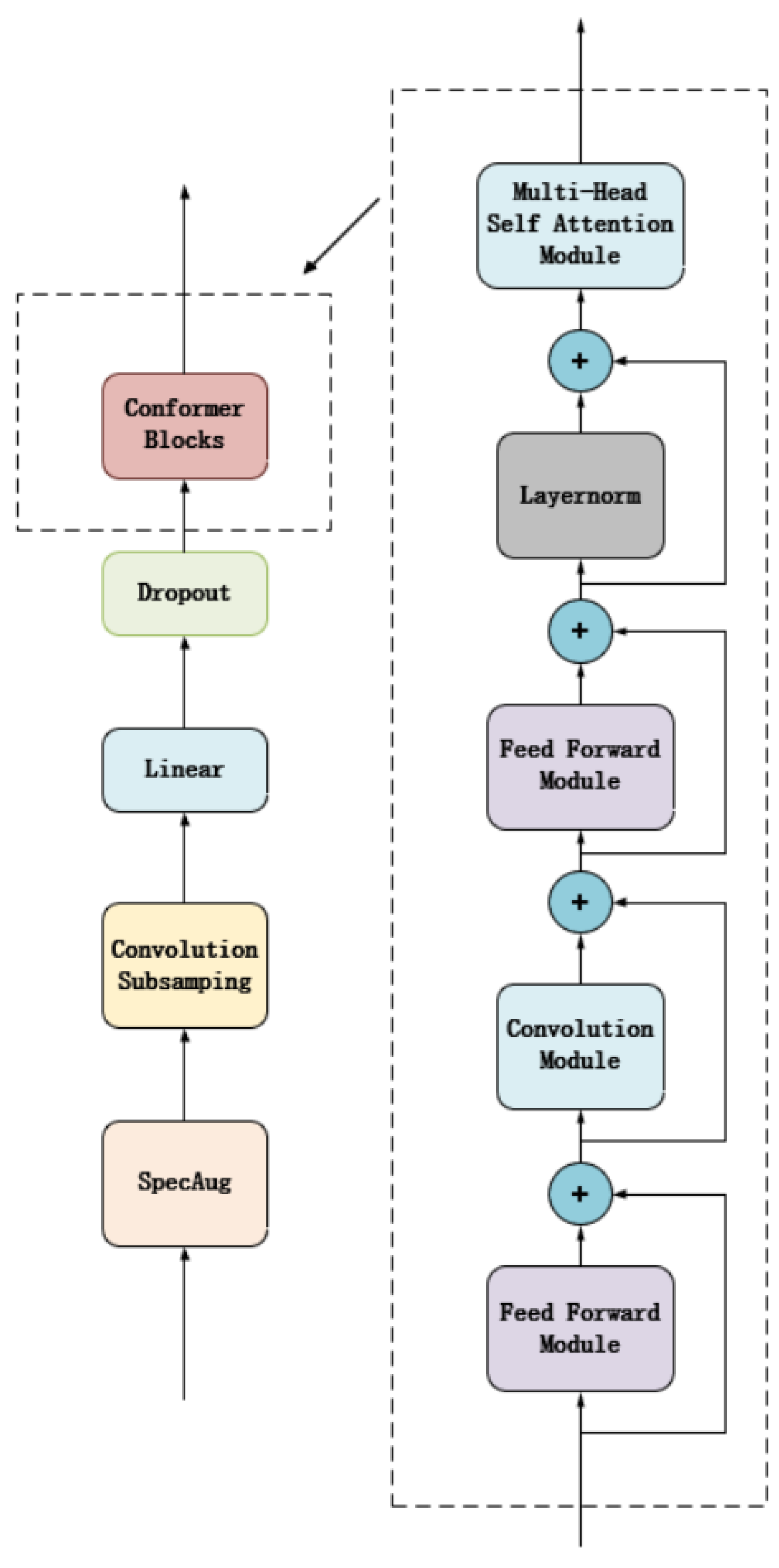
The Conformer structure is a deep-learning architecture that combines self-attention mechanisms and convolutional neural networks, mainly used for processing time series tasks. It was proposed by Anmol Gulati and other researchers in 2020 [16]. The Conformer structure typically includes several key parts: self-attention layers, convolutional neural networks, and feedforward networks. These components interact with each other in a specific way within the module to improve processing efficiency and model performance. The self-attention mechanism helps the model capture long-term dependencies in time series data, while the convolutional layers capture local features, and the feedforward network further transforms features, adding nonlinear processing capabilities to enhance the overall expressiveness of the model. This combination makes Conformer very suitable for processing time series data. Figure 1 shows the structure diagram of Conformer.

In the self-attention layer, the model no longer relies on traditional sequence processing methods, such as Recurrent Neural Networks (RNN), which process information step by step, but directly captures the interactions between all elements in the sequence by calculating the weight distribution of all element pairs [18]. This mechanism is achieved by generating three vectors, query, key, and value, and calculating the compatibility score between the query and all keys. The values corresponding to the keys with high scores will have a greater influence. This processing method allows for each sequence element to “pay attention” to the other elements directly, thereby dynamically focusing on the information most important for the current task.

The design of the feedforward network is to increase the model’s nonlinear processing capability and transform high-dimensional features, thereby enhancing the learning model’s expressive power and generalizability. In terms of computation, the feedforward network is usually composed of two densely connected linear layers, with a nonlinear activation function, such as ReLU (Rectified Linear Unit) or GELU (Gaussian Error Linear Unit), embedded in the middle. The purpose of this configuration is to introduce the necessary nonlinearity, allowing for the network to learn and approximate complex functional relationships.

2.2. Convolutional Neural Networks

The basic composition of Convolutional Neural Networks includes convolutional layers, pooling layers, and fully connected layers. Convolutional layers use a set of learnable filters, each of which is responsible for extracting local features of the input data [19]. By sliding these filters on the input data, a series of activation maps (also known as feature maps) are generated, which encode important spatial features of the input data. The effectiveness of convolutional operations lies in their local connectivity and weight sharing, allowing for the network to process large images with fewer parameters.

Pooling layers are located between consecutive convolutional layers, and their main function is to reduce the spatial dimensions of feature maps, thereby reducing the number of parameters and computational cost of subsequent layers. Pooling operations are achieved by extracting statistical information within local areas (usually the maximum or average value), which not only helps to make the feature representation more compact but also enhances the model’s robustness to small positional changes.

Fully connected layers are usually located at the end of the network, and their task is to perform final classification or regression analysis based on the features extracted and integrated by the previous layers. Each fully connected layer converts the output of the previous layer into a higher-level representation, and the last fully connected layer outputs the final prediction result.

2.3. LSTM

Long Short-Term Memory networks (LSTM) [17] are an advanced type of Recurrent Neural Network (RNN) designed to handle time series data with long-term dependencies. Since their introduction by Hochreiter and Schmidhuber in 1997, LSTMs have become one of the standard tools for dealing with time series problems, especially in applications that require understanding and predicting long-term data patterns.

The core innovation of LSTM lies in its unique gating mechanism, which includes input gates, forget gates, and output gates. These mechanisms work together to manage the flow of information between cells. This design allows for the network to retain important historical information while forgetting irrelevant data, effectively addressing the problem of gradient disappearance or explosion faced by traditional RNNs when processing long sequences. In addition, the cell state in LSTM serves as a carrier of information, running through the entire sequence, ensuring that key information can be preserved and utilized in the time series. The core structure of the LSTM is shown in Figure 2.

Through these gating mechanisms and memory cell designs, LSTM networks can effectively capture long-term dependencies.

2.4. Spearman Correlation Analysis

Spearman correlation analysis is a non-parametric statistical method used to assess the monotonic relationship between two variables [20]. Unlike Pearson correlation, Spearman correlation does not require data to meet the normal distribution assumption and is suitable for dealing with non-linear relationships, thus improving the robustness of the analysis [21].

The Spearman correlation coefficient ρ can be expressed as follows [20]:

$$\mathit{\rho }=1-\frac{6{{\displaystyle \sum }}^{}{{\mathit{d}}_{\mathit{i}}}^2}{\mathit{n}\left({\mathit{n}}^2-1\right)}$$

(1)

where ${\mathit{d}}_{\mathit{i}}$ is the difference in rank between the two variables and n is the number of data points. $\mathit{\rho }$ > 0 indicates a perfect positive correlation, and $\mathit{\rho }$ < 0 indicates a perfect negative correlation.

An important advantage of Spearman correlation analysis is its insensitivity to outliers and non-linear relationships. This makes it more stable and reliable when dealing with data that include outliers or non-linear relationships. In addition, due to its non-parametric nature, Spearman correlation does not depend on the specific distribution of the data, which is particularly important in practical applications of wave height prediction.

2.5. Algorithm Design Ideas

This study proposes a Conformer-LSTM model that uses Spearman correlation analysis on common buoy data (wind speed, air temperature, atmospheric pressure, wave period) and selects features with high correlation to the target feature of wave height, such as wind speed [22], temperature [23], atmospheric pressure [24], and wave period [25], as parameters for training.

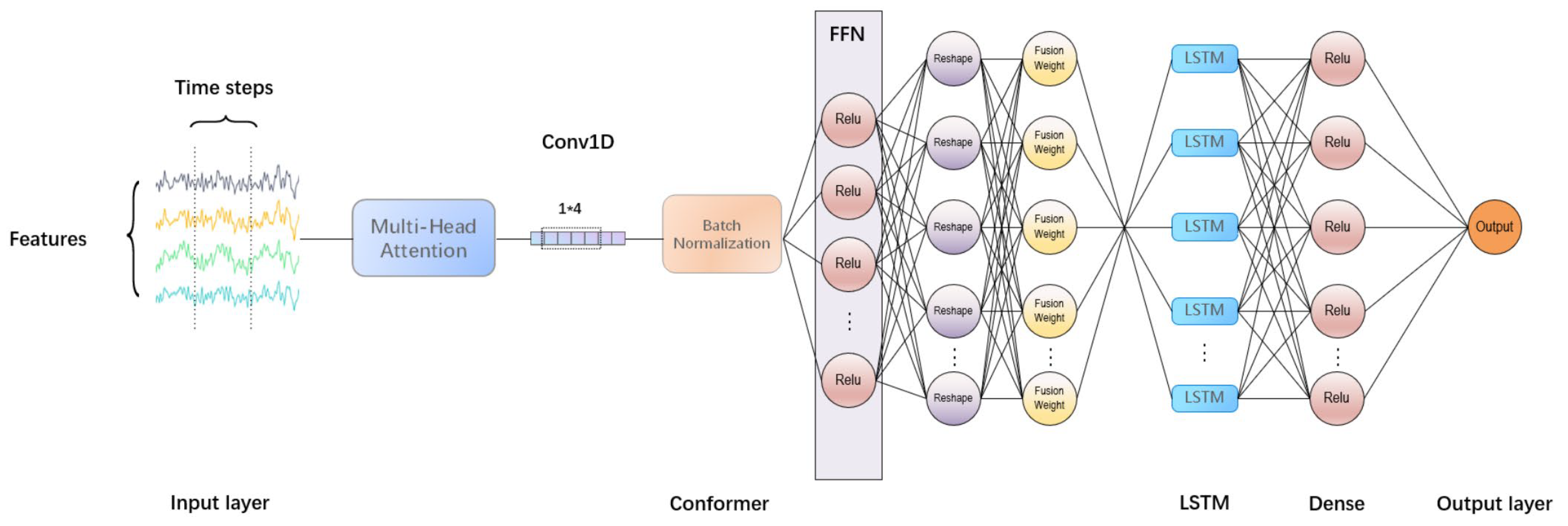
This paper uses multi-head attention mechanisms to obtain the global dependencies of the data and combines convolutional layers to capture local features. Batch normalization [26] is used to normalize the output, reducing internal covariate shift. An adaptive feature fusion weight network is introduced, allowing for the model to dynamically adjust the fusion weights of different features according to the characteristics of the input data. Finally, a Long Short-Term Memory network is used to capture long-term dependencies in the data for prediction, reducing errors and improving prediction accuracy.

2.6. Algorithm Process

The flowchart of our algorithm shows in the Figure 3.

We used Spearman correlation analysis on buoy data to select feature variables with high correlation to wave height. The results are given in

Table 1. Explanation of buoy data.

Features	Explanation
WVHT	Significant wave height (meters) is calculated as the average of the highest one-third of all of the wave heights during the 20 min sampling period.
WSPD	Wind speed (m/s) averaged over an eight-minute period for buoys.
GST	Peak 5 or 8 s gust speed (m/s) measured during the eight-minute or two-minute period.
ATMP	Air temperature (Celsius)
WTMP	Sea surface temperature (Celsius).
DEWP	Dewpoint temperature taken at the same height as the air temperature measurement.
APD	Average wave period (seconds) of all waves during the 20 min period.
DPD	Dominant wave period (seconds) is the period with the maximum wave energy.

and

Table 2. Correlation coefficients based on multi-variable features at station 41040 in 2021, with the target variable being wave height.

Feature Name	WSPD	GST	ATMP	WTMP	DEWP	APD	DPD	PRES
Correlation Coefficient	0.662	0.689	−0.330	0.112	−0.310	0.595	0.294	0.104

.

The correlation coefficient ranges from [−1, 1]. The closer the absolute value of the coefficient is to 1, the higher the correlation; the closer to 0, the lower the correlation. A negative value indicates a negative correlation with the target feature.

Experiments show that, in terms of wind speed, although GST has a higher correlation than WSPD, GST is an instantaneous value, while the target feature of wave height to be predicted is an average value. Therefore, WSPD is selected as the feature variable for wind speed; in terms of temperature, ATMP has a higher correlation than WTMP and DEWP, so ATMP is selected as the temperature feature variable; in terms of wave period, APD has a significantly higher correlation than DPD; finally, the atmospheric pressure value at sea level is selected as the pressure feature variable.

Enter the Conformer, using multi-head self-attention mechanisms to transform the input X, generating different query (Q), key (K), and value (V) vectors for each head:

$${\mathit{Q}}_{\mathit{i}}=\mathit{X}{\mathit{W}}_{\mathit{i}}^{\mathit{Q}}$$

(2)

$${\mathit{K}}_{\mathit{i}}=\mathit{X}{\mathit{W}}_{\mathit{i}}^{\mathit{K}}$$

(3)

$${\mathit{V}}_{\mathit{i}}=\mathit{X}{\mathit{W}}_{\mathit{i}}^{\mathit{V}}$$

(4)

where ${\mathit{W}}_{\mathit{i}}^{\mathit{Q}}, {\mathit{W}}_{\mathit{i}}^{\mathit{K}},\mathrm{and} {\mathit{W}}_{\mathit{i}}^{\mathit{V}}$ are learnable weight matrices, corresponding to the query, key, and value of the i-th head, respectively.

Calculate the scaled dot-product attention for each head [27]:

$$\mathit{A}\mathit{t}\mathit{t}\mathit{e}\mathit{n}\mathit{t}\mathit{i}\mathit{o}\mathit{n}({\mathit{Q}}_{\mathit{i}},{\mathit{K}}_{\mathit{i}},{\mathit{V}}_{\mathit{i}})=\mathit{s}\mathit{o}\mathit{f}\mathit{t}\mathit{m}\mathit{a}\mathit{x}(\frac{{\mathit{Q}}_{\mathit{i}}{\mathit{K}}_{\mathit{i}}^{\mathit{T}}}{\sqrt{{\mathit{d}}_{\mathit{k}}}}){\mathit{V}}_{\mathit{i}}$$

(5)

Enter the one-dimensional convolutional layer, using a sliding window to extract the feature relationships between samples, and use a one-dimensional convolutional kernel with a length of 5 (the same as the number of feature values) to extract features. This method can focus on potential trends in the data within a short period.

During the training of deep neural networks, the input distribution of each layer changes due to parameter updates in the previous layer. This phenomenon is called “internal covariate shift.” To reduce this shift, batch normalization normalizes the input of each layer, ensuring that their mean is 0 and variance is 1. This normalization helps the model converge faster and improves its generalization ability.

For a given batch of data, calculate the mean of each feature [26]:

$$\mathit{\mu }=\frac{1}{\mathit{m}}{{\displaystyle \sum }}_{\mathit{i}=1}^{\mathit{m}}{\mathit{x}}_{\mathit{i}}$$

(6)

Calculate the variance of each feature:

$${\mathit{\sigma }}^2=\frac{1}{\mathit{m}}{{\displaystyle \sum }}_{\mathit{i}=1}^{\mathit{m}}{\left({\mathit{x}}_{\mathit{i}}-\mathit{\mu }\right)}^2$$

(7)

$${\widehat{\mathit{x}}}_{\mathit{i}}=\frac{{\mathit{x}}_{\mathit{i}}-\mathit{\mu }}{\sqrt{{\mathit{\sigma }}^2+\mathit{ϵ}}}$$

(8)

where $\mathit{ϵ}$ is a small number to avoid division by 0.

$${\mathit{y}}_{\mathit{i}}=\mathit{\gamma }{\widehat{\mathit{x}}}_{\mathit{i}}+\mathit{\beta }$$

(9)

where $\mathit{\gamma } \mathrm{and} \mathit{\beta }$ are scale and shift parameters, respectively, obtained through training.

In Figure 4, batch normalization is applied to the output of the convolutional layer, which helps with the stability and convergence speed during the model training process. Three dense layers are used, with the first dense layer using the ReLU activation function to process the output of the convolutional layer, adding nonlinear processing capabilities. The second dense layer is used to adjust the input dimensions to match the added output of the adjusted feedforward network. The third dense layer calculates the weight of each input feature through learning, which is used to adjust the output of the feedforward network to emphasize more important features.

An LSTM layer is used to process the output of the Conformer block. The LSTM layer is configured with 32 units, does not return a sequence, and only returns the output of the last time step. LSTM can handle long-term dependencies in time series, and its gating mechanism helps the model remember and forget information, thereby capturing dynamic changes in time series data.

By combining Conformer and LSTM, the model leverages the strengths of both architectures. The Conformer’s self-attention mechanism effectively captures spatial relationships and temporal dynamics, while the LSTM ensures that long-term dependencies are adequately managed. This hybrid approach results in a model that is better equipped to handle the complex, non-linear, and dynamic nature of ocean wave data.

The final output section includes a flattening layer followed by two dense layers. The flattening layer converts the output of the LSTM into a one-dimensional array to meet the input requirements of the fully connected layer. The first dense layer uses the ReLU activation function, and the second one directly outputs the predicted result without an activation function. The dense layer is responsible for mapping the processed features to the final predicted target.

2.7. Dataset

The data come from the buoy data of the National Oceanic and Atmospheric Administration (NOAA) NDBC, mainly distributed in the North Atlantic, Pacific, and Gulf of Mexico near North America.

Table 3. Site information.

Site Name	Longitude	Latitude	Water Depth	Time Range
41048	69°34′23″ W	31°49′53″ N	5394 m	1 January 2021–31 December 2021
46047	119°31′30″ W	32°23′18″ N	1423 m	1 January 2022–31 December 2022
41040	53°8′11″ W	14°32′9″ N	4988 m	1 January 2020–31 December 2020
42020	96°41′12″ W	26°57′18″ N	84 m	1 January 2022–31 December 2022
42057	81°34′31″ W	16°58′22″ N	412 m	1 January 2020–12 December 2020
46025	119°2′42″ W	33°45′19″ N	890 m	1 January 2022–31 December 2022
42002	93°38′46″ W	26°3′18″ N	3088 m	1 January 2022–31 December 2022

covers different water depths to verify the generalization of the model. The buoy data have a sampling interval of one hour, and the site information used in this experiment is shown in the Table 3 and Figure 5.

When selecting sites, we chose different sites located in the Gulf of Mexico, along the Pacific coast, and along the Atlantic coast. Similarly, the sea areas of these sites have different depths. The shallowest depth we selected is 84 m, and the deepest is 5394 m. Depth has a certain impact on wave height, and the depth at the location of the same buoy will not change. We hope the diversity of depth and location can prove the generalizability of our model.

Since the raw wave data directly obtained contain a small number of missing values, the existence of these missing values can make the prediction accuracy and generalization performance poor. Therefore, it is necessary to first interpolate the missing data using the previous and next moment data.

Table 4. The number of missing data in each site.

Site Name	Number of Missing Data	Number of Total Data	Missing Rate (%)
41048	63	8596	0.73
46047	99	8757	1.13
41040	112	8710	1.28
42020	146	8751	1.66
42057	110	8252	1.33
46025	128	8748	1.46
42002	103	8756	1.17

shows the number and percentage of missing values in the selected datasets. The number of missing values is relatively small because we prioritized selecting sites with sufficient data when choosing our dataset. If a site had too many missing values, it would significantly affect our predictions.

Since the units of wave height, wind speed, and air temperature are different and the numerical values vary greatly, direct use in training will lead to unfair calculation of data, so the original data are normalized using the minimum–maximum method, mapping all feature data to the interval (0, 1), ensuring that all features are treated fairly during the training process of the fusion model and improving the prediction accuracy.

The specific formula is as follows (10) [28]:

$$\tilde{\mathit{x}}=\frac{\mathit{x}-{\mathit{x}}_{\mathit{m}\mathit{i}\mathit{n}}}{{\mathit{x}}_{\mathit{m}\mathit{a}\mathit{x}}-{\mathit{x}}_{\mathit{m}\mathit{i}\mathit{n}}}$$

(10)

Considering the needs of time series forecasting, this study constructs training and testing time series datasets through the sliding window method. Each data instance consists of 24 consecutive time steps, which are used to predict the wave height of the next time step. For each time point, the data of the previous 24 time points are used as input features, and the wave height of the next time point is used as the target output. Each group of samples includes four feature values, which are wave height, wind speed, air temperature, and atmospheric pressure.

During the training process, the dataset is divided into a training set and a test set, with 80% of the data used for model training and the remaining 20% used for model performance evaluation.

2.8. Evaluation Criteria

This experiment uses MAE, RMSE, MAPE, and ${\mathit{R}}^2$ as evaluation indicators to measure the accuracy of the model, and the specific formulas for each evaluation indicator are as follows [29].

MAE (Mean Absolute Error) is another commonly used indicator to measure the difference between the predicted model and the actual results. MAE calculates the average of the absolute values of the differences between predicted and actual values.

$$\mathit{M}\mathit{A}\mathit{E}=\frac{1}{\mathit{n}} {\displaystyle \sum }_{\mathit{i}=1}^{\mathit{n}}\mid {\mathit{y}}_{\mathit{i}}-{\widehat{\mathit{y}}}_{\mathit{i}}\mid$$

(11)

The smaller the MAE, the higher the prediction accuracy of the model.

RMSE (Root Mean Square Error) is a commonly used indicator to measure the difference between the model’s predicted results and the actual data. Its calculation method is to first calculate the square of the difference between each predicted value and the actual value, then take the average of all the squared differences, and finally take the square root of this average value.

$$\mathit{R}\mathit{M}\mathit{S}\mathit{E}=\sqrt{\frac{1}{\mathit{n}}{\displaystyle \sum }_{\mathit{i}=1}^{\mathit{n}}{\left({\mathit{y}}_{\mathit{i}}-{\widehat{\mathit{y}}}_{\mathit{i}}\right)}^2}$$

(12)

The smaller the RMSE value, the closer the model’s predicted results are to the actual data, and the better the model’s prediction performance.

MAPE (Mean Absolute Percentage Error) is an indicator used to measure the accuracy of the prediction model, which expresses the error between the predicted value and the actual value in percentage form.

$$\mathit{M}\mathit{A}\mathit{P}\mathit{E}=\frac{1}{\mathit{n}} {{\displaystyle \sum }}_{\mathit{i}=1}^{\mathit{n}}\mid \frac{{\mathit{y}}_{\mathit{i}}-{\widehat{\mathit{y}}}_{\mathit{i}}}{{\mathit{y}}_{\mathit{i}}}\mid$$

(13)

The smaller the MAPE value, the higher the prediction accuracy of the model.

The coefficient of determination, also known as the goodness of fit, reflects the quality of the model’s fit. Its result is between 0 and 1.

$${\mathit{R}}^2\left(\mathit{y},\widehat{\mathit{y}}\right)=1-\frac{{{\displaystyle \sum }}_{\mathit{i}=1}^{\mathit{n}}{\left({\mathit{y}}_{\mathit{i}}-{\widehat{\mathit{y}}}_{\mathit{i}}\right)}^2}{{{\displaystyle \sum }}_{\mathit{i}=1}^{\mathit{n}}{\left({\mathit{y}}_{\mathit{i}}-{\overline{\mathit{y}}}_{\mathit{i}}\right)}^2}$$

(14)

The closer the coefficient of determination is to 1, the higher the prediction accuracy of the model.

$y_i$ is the true value of the i-th prediction sample; ${\widehat{y}}_i$ is the predicted value of the i-th prediction sample;${\overline{y}}_i$ is the mean value of the actual values of the prediction samples; and N is the total number of prediction samples.

2.9. Software Environment

The hardware environment of this experiment includes an i7-9750H CPU, an RTX 2060 GPU, and 16 GB of memory. The software environment includes the Windows 10 version 21H2 operating system, PyCharm version 2025.1.4 development software, and TensorFlow v2.16.1 framework.

3. Results and Discussion

3.1. Performance of Conformer-LSTM

The model is used to predict wave height data using a sliding window method to predict the wave height of the twenty-fifth hour with data from every 24 h of feature variables. The prediction performance of the model is analyzed using MAE, RMSE, and MAPE as evaluation indicators for each station’s prediction data. When using the Conformer-LSTM algorithm for prediction, the training parameters are set to epochs = 100 and batch_size to 16, with a learning rate of 0.001.

Table 5. Prediction Results for Stations 41048 and 46047.

Station Name	Network Name	MAE	RMSE	MAPE (%)	R2
41048	Conformer-LSTM	0.12909	0.17745	5.4335	0.95961
	LSTM	0.15055	0.20797	7.1349	0.94629
46047	Conformer-LSTM	0.11975	0.13394	4.829	0.96392
	LSTM	0.12829	0.14713	4.9998	0.95843

provides a preliminary view in which the Conformer-LSTM model shows better performance in predicting wave heights compared to traditional models.

In the table, we can initially observe that the Conformer-LSTM model performs better than the LSTM model at these two sites, providing preliminary evidence that the Conformer-LSTM model has improved prediction accuracy.

To further demonstrate the predictive performance of the model, line charts are used to compare the predicted and actual values, as shown in the figures. The model shows good fitting effects.

Observing Figure 6 and Figure 7, we find that the Conformer-LSTM model’s prediction results have a good fitting effect with the actual wave heights.

3.2. Generalization Performance of the Model

To further prove the generalization performance of the model, more stations are introduced for prediction. The Conformer-LSTM is used to predict stations 41040 and 42020.

Analyzing more sites,

Table 6. Prediction results for stations 41040 and 42020.

Station Name	Network Name	MAE	RMSE	MAPE (%)	R2
41040	ConformerLSTM-WaveNet	0.08856	0.11708	4.2548	0.95025
	LSTM	0.09194	0.12029	4.457	0.94748
42020	ConformerLSTM-WaveNet	0.09719	0.15381	5.8291	0.97768
	LSTM	0.11294	0.17244	6.3098	0.96875

shows that the Conformer-LSTM model performs better than the LSTM model at these two sites, further proving that the Conformer-LSTM model has improved prediction accuracy.

3.3. Comparison with Other Models

Table 7. Evaluation results of different models at different stations.

Station	Network	MAE	RMSE	MAPE (%)	R2
41048	Conformer-LSTM	0.12909	0.17745	5.4335	0.95961
	LSTM	0.15055	0.20797	7.1349	0.94629
	CNN	0.16022	0.22598	8.4804	0.93658
	CNN-LSTM	0.13436	0.18544	5.5754	0.9559
	BiLSTM	0.13959	0.18937	5.9103	0.95401
	TCN	0.16594	0.23518	6.8163	0.92906
46047	Conformer-LSTM	0.11975	0.13394	4.829	0.96392
	LSTM	0.12829	0.14713	4.9998	0.95843
	CNN	0.13453	0.15836	5.2322	0.95135
	CNN-LSTM	0.125363	0.14936	4.9756	0.95829
	BiLSTM	0.134413	0.16914	4.8314	0.95314
	TCN	0.14719	0.1795	5.7141	0.92668
41040	Conformer-LSTM	0.08856	0.11708	4.2548	0.95025
	LSTM	0.09194	0.12029	4.457	0.94748
	CNN	0.09087	0.12977	4.3603	0.94794
	CNN-LSTM	0.09481	0.13303	4.6166	0.94507
	BiLSTM	0.09021	0.12931	4.307	0.94834
	TCN	0.09051	0.12693	4.4491	0.94752
42020	Conformer-LSTM	0.09719	0.15381	5.8291	0.97768
	LSTM	0.11294	0.17244	6.3098	0.96875
	CNN	0.12118	0.19562	6.8437	0.9657
	CNN-LSTM	0.10647	0.17988	6.7574	0.96987
	BiLSTM	0.10418	0.18021	6.4032	0.97389
	TCN	0.14089	0.20168	7.2607	0.95252
42057	Conformer-LSTM	0.08045	0.12654	6.0541	0.97452
	LSTM	0.08873	0.13230	6.8501	0.96520
	CNN	0.09054	0.14565	6.5521	0.96014
	CNN-LSTM	0.08245	0.12975	6.4532	0.96745
	BiLSTM	0.10451	0.15325	7.2523	0.95412
	TCN	0.09514	0.14547	6.8514	0.96123
46025	Conformer-LSTM	0.11123	0.14576	5.4541	0.96741
	LSTM	0.13574	0.16345	6.2414	0.95245
	CNN	0.14537	0.17632	6.8544	0.94951
	CNN-LSTM	0.11954	0.15016	5.8541	0.96247
	BiLSTM	0.13246	0.16854	6.2484	0.95126
	TCN	0.14767	0.19754	7.2541	0.94254
42002	Conformer-LSTM	0.09451	0.15461	6.6554	0.96314
	LSTM	0.10004	0.16275	7.0541	0.95445
	CNN	0.10547	0.16345	7.2964	0.95521
	CNN-LSTM	0.09679	0.15778	6.8471	0.95842
	BiLSTM	0.11047	0.16547	7.2333	0.95124
	TCN	0.11245	0.17571	8.5114	0.94897

lists the prediction effects of Conformer-LSTM, LSTM, CNN, CNN-LSTM, BiLSTM [30], and TCN [31] at stations 41048, 46047, 41040, and 42020, showing that Conformer-LSTM has better performance.

This table provides the accuracy obtained using different prediction algorithms at all sites. By observing the table, we find that the Conformer-LSTM model achieves better performance at each site.

By analyzing and comparing the average accuracy data obtained in

Table 8. Accuracy improvement of Conformer-LSTM compared to other networks.

Network	MAE	RMSE	MAPE (%)	R2
LSTM	10.82%	8.78%	10.54%	0.95%
CNN	15.02%	15.56%	15.58%	1.35%
CNN-LSTM	5.13%	7.02%	6.25%	0.58%
BiLSTM	11.65%	12.65%	8.71%	1.05%
TCN	19.89%	20.0.%	17.81%	2.24%

, it can be found that the Conformer-LSTM model shows varying degrees of improvement over other traditional models.

In this study, we utilized data from two buoys located in the Gulf of Mexico and two in the Pacific Ocean. While these buoys provided valuable data for our analysis, it is important to note that the limited number of buoys and their close proximity in the Pacific Ocean could constrain the generalizability of our findings. Future studies should consider incorporating data from a larger number of buoys distributed more widely across different oceanic regions to enhance the robustness of the predictions.

4. Conclusions

This study proposes a hybrid model (Conformer-LSTM) based on Conformer and LSTM for wave height prediction. By introducing the self-attention mechanism and convolutional layer from Conformer combined with LSTM’s processing of long-term dependencies in time series data, the model shows excellent performance in capturing non-linear features and dynamic changes in time series data. At the same time, the use of an adaptive feature fusion weight network enhances the model’s recognition and utilization efficiency of key features.

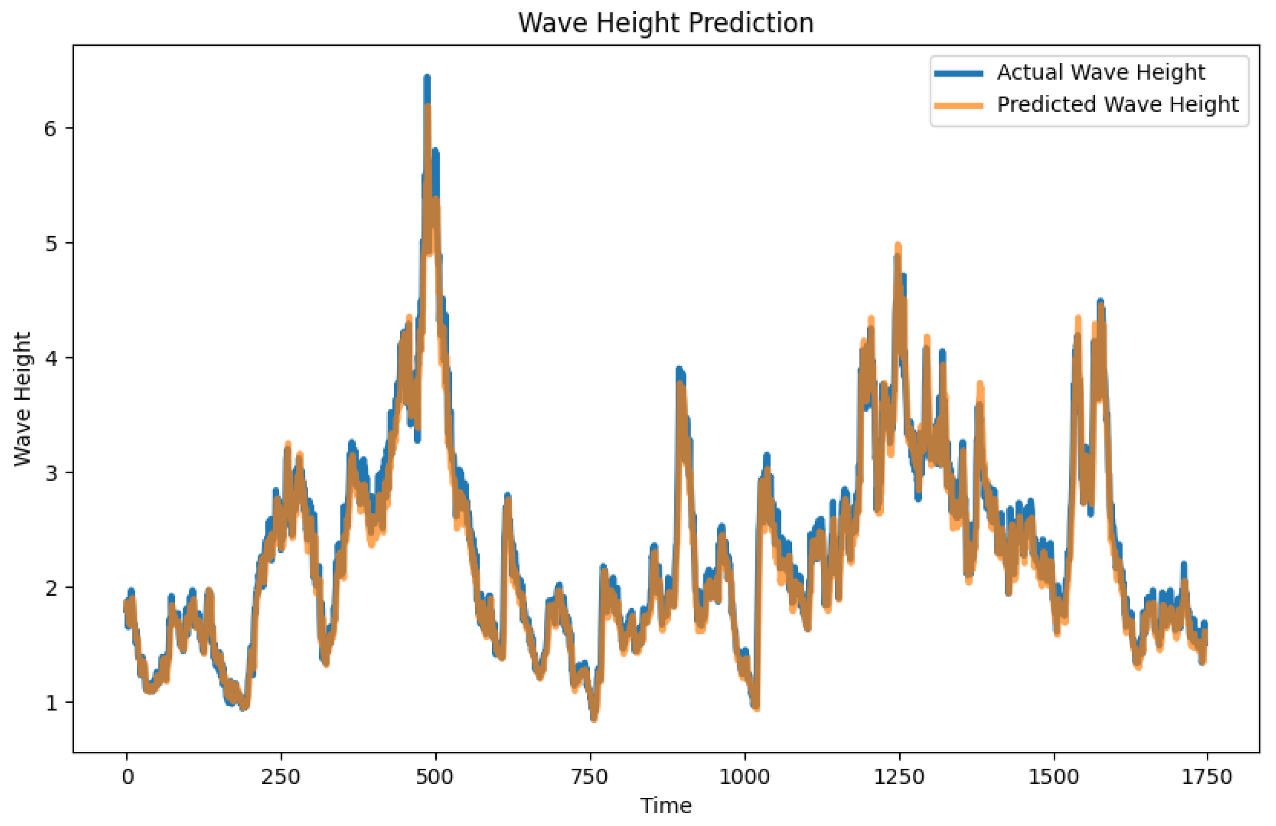
Experimental data come from the National Oceanic and Atmospheric Administration (NOAA) NDBC buoy data, and evaluation indicators include Mean Absolute Error (MAE), Root Mean Square Error (RMSE), Mean Absolute Percentage Error (MAPE), and Coefficient of Determination (R²). The experimental results show that the Conformer-LSTM model performs better than traditional LSTM, CNN, and CNN-LSTM models at multiple stations, confirming its potential in wave height prediction.

The CNN-LSTM model proposed by Guan [14] showed better performance compared to standalone LSTM and random forest models. Despite these improvements, our Conformer-LSTM model demonstrated a higher accuracy in both short-term and medium-term wave height predictions, as evidenced by lower MAPE and higher R² values.

Through comparative analysis of the prediction effects of different models, it can be observed that the Conformer-LSTM model has a significant advantage in capturing complex time series features, especially in dealing with nonlinear and non-stationary wave data, showing higher prediction accuracy and robustness. Further verification of the prediction effects at more stations demonstrates the model’s generalization ability and practicality.

The implications of accurate wave height prediction extend beyond maritime safety. Reliable forecasts contribute to the economy by optimizing shipping routes, reducing fuel consumption, and minimizing the risk of maritime accidents. This, in turn, can lower insurance costs and enhance the overall efficiency of maritime logistics. Furthermore, precise wave height predictions support coastal zone management and the planning of offshore operations, contributing to the sustainable development of marine resources and the protection of coastal infrastructure.

In terms of societal impact, improved wave height prediction models can enhance disaster preparedness and response. Early warnings of extreme wave events can save lives and reduce property damage in coastal communities. Additionally, accurate wave forecasts support recreational activities and tourism, ensuring safety and enhancing the experience for those engaging in water sports and coastal tourism.

However, this study also has some limitations. This model is specifically designed to handle non-linear, medium- to long-period data, making it particularly suitable for scenarios where such characteristics are prominent. However, the model may not perform as well with data that are primarily linear or exhibit very short-term periodicity.

Another limitation of this study is the small number of buoys used for data collection. Future research should aim to include a greater number of buoys, potentially in diverse geographical locations, to validate and extend the applicability of the proposed method. Focusing on a single location with a more significant number of data points could provide additional validation and improve the generalizability of the results.

Future research will aim to address the limitations identified in this study by incorporating data from a larger number of buoys spread across diverse geographical locations. This would enhance the generalizability of the wave height predictions. Additionally, focusing on single locations with a greater number of data points could provide more comprehensive validation of the proposed method. Further exploration into optimizing the computational efficiency of the model and adapting it to different sea areas would also be beneficial.

In addition, the model training process requires a lot of computing resources and time. How to optimize the computational efficiency of the model is a direction for future research.