Improved CycleGAN for Mixed Noise Removal in Infrared Images

Abstract

Infrared images are susceptible to interference from a variety of factors during acquisition and transmission, resulting in the inclusion of mixed noise, which seriously affects the accuracy of subsequent vision tasks. To solve this problem, we designed a mixed noise removal algorithm for infrared images based on improved CycleGAN. First, we proposed a ResNet-E Block that incorporates the EMA (Efficient Multi-Scale Attention Module) and build a generator based on it using the skip-connection structure to improve the network’s ability to remove mixed noise of different strengths. Second, we added the PSNR (Peak Signal-to-Noise Ratio) as an extra calculation item of cycle consistency loss, so that the network can effectively retain the detailed information of infrared images while denoising. Finally, we conducted experimental validation on both synthetic noisy images and real noisy images, which proved that our algorithm can effectively remove the mixed noise in infrared images and the denoising effect is better than other similar methods.

1. Introduction

In recent years, the demand for image information has increased significantly, which has greatly promoted the rapid development of various imaging technologies [1]. Imaging modalities based on optical sensors are unable to meet the needs of all-weather imaging missions due to the constraints imposed by factors such as ambient light. The imaging technology based on infrared sensors mainly relies on the infrared radiation of the object for imaging [2], so it is not affected by natural conditions such as light, rainfall or haze, and is widely used in industrial monitoring, medical diagnosis, remote sensing observation and national defense [3]. However, external interference during the imaging process, the electrical characteristics of the infrared device itself and the compression degradation during the image transmission and processing led to infrared images inevitably being corrupted by random signals and containing mixed noise [4]. The existence of mixed noise will cause the image to contain erroneous or redundant pixel values, which will blur it from visual perception and cover up the real feature information of the object, thus affecting the accuracy of subsequent advanced visual tasks. Therefore, denoising is often a primary and essential step in the use of infrared images.

Based on the uncorrelation between the real signal pixels and the noise pixels in the image, most of the traditional infrared image denoising methods use the idea of filtering and transforming as the design basis of the algorithm [5]. Accompanied by the progress of signal processing theories over the past few decades, traditional denoising methods have gradually developed and matured, and a large number of derived methods have been produced. According to the different processing domains, these methods can be categorized into spatial-based methods, transform-based methods and spatial combined with transform methods [6]. Spatial-based denoising methods utilize the correlation between neighboring real pixels of an image and process the pixel values directly on the original image to recover the information masked by noise, and the typical algorithms mainly include mean filtering [7], median filtering [8], Gaussian filtering [9] and bilateral filtering [10]; the transform-based methods remove noise by transforming the image into the frequency domain or wavelet domain and inverting the result back to the image domain by processing the relevant parameters, and representative algorithms mainly include Discrete Fourier Transform [11], Wavelet Transform [12] and Discrete Cosine Transform [13]; image denoising methods based on the spatial combined with transform method achieve better denoising effect by combining the relevant algorithms in the spatial and transform domains, which comprehensively utilize the advantages of both to overcome the limitations of each. It mainly includes the BM3D (Block Matching and 3D collaborative filtering) [14] algorithm and the WNNM (Weighted Nuclear Norm Minimization) [15] algorithm.

Although the traditional methods started earlier and provided a variety of generalized algorithms for the denoising task of infrared images for a long time, with the proposal of deep learning networks and their wide application in the field of image processing, algorithms based on deep learning have further pushed forward the development of denoising methods for infrared images and gradually become the mainstream of the current denoising approaches [16]. Compared with traditional algorithms, methods based on deep learning achieve better denoising results and the models obtained through training have a greater ability to generalize the inference of new concepts and get good performance on unfamiliar data or tasks. However, these methods still suffer from ineffective removal of mixed noise and loss of image texture details due to denoising. In order to address the above shortcomings, some researchers have made improvements on the original deep learning networks. For example, [17] proposed an infrared image noise removal network called the DMD-CNN (Deep Multi-scale Dense connection Convolutional Neural Network), which contains a multi-scale feature representation unit that can decompose the image into different scales for effective utilization of image information. In addition to this, dense link structure and regularization terms are introduced in the network to reconstruct the smoothness in the vertical direction of the information containing the noise; [18] proposed an infrared image denoising enhancement method called IE-CGAN (Image Enhancement Conditional Generative Adversarial Network), which realizes the linear combination of feature information in the learning process of the network by adding the skip-connection structure to link the relevant feature mapping layers in the generator, while the discriminator network adopts an all-CNN structure to convert the input image into smaller feature mappings and enhance its discriminative ability to promote the generator to produce better denoised images. An algorithm called DestripeCycleGAN infrared image denoising algorithm is presented in [19], which uses a MWUNet (Multi-level Wavelet U-Net) as a denoising generator and utilizes Haar wavelet transform as a sampler to reduce the loss of orientation information. In addition, the algorithm combines GFB (Group Fusion Block) in the form of skip connections to realize the fusion of multi-scale feature information. The authors of [20] combined residual block, non-local attention and bicubic interpolation to form a MLFAB (Multi-level Feature Attention Block), and added it to the generator structure of GAN to propose a MLFAN (Multi-level Feature Attention Network) for the task of denoising infrared images, which is capable of effectively removing Gaussian noise, Poisson noise and the mixture of the two from the image. At the same time, the MLFAB module fuses higher-order and lower-order feature information, which enhances the ability to retain the details of the image.

Inspired by the work of the above researchers, this paper presents a mixed noise removal method for infrared images based on improved CycleGAN, and the main contributions can be summarized as follows:

(1)

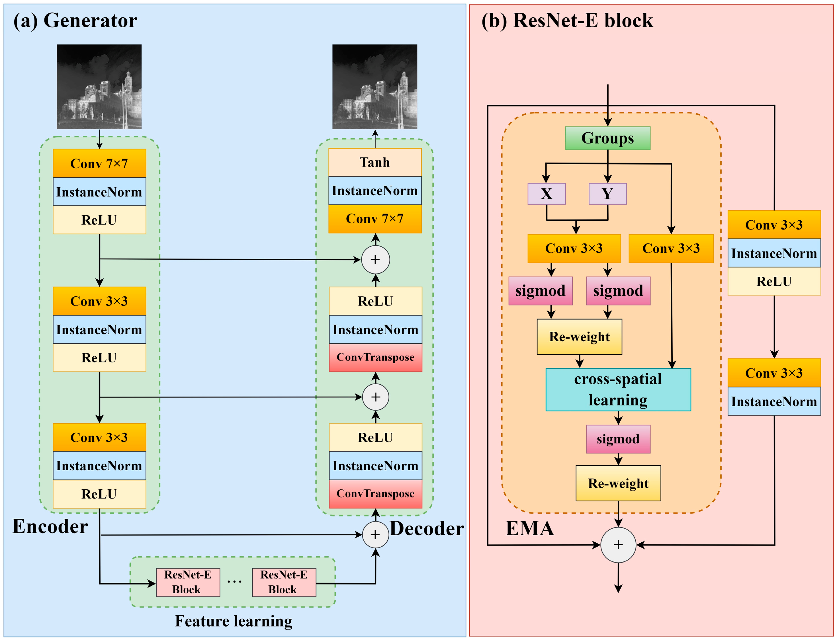
By adding the EMA attention mechanism to the traditional residual module structure, a Resnet-E feature extraction module is proposed, and a generator is designed based on this module using the skip-connection structure, which improves the denoising performance of the network for mixed noises.

(2)

A new term containing PSNR loss calculation is added to the original cycle consistency loss function, which better ensures the consistency of the non-noise features between the input image and the output image, and thus improves the network’s ability to retain details when removing noise.

(3)

Experimental validation on both synthesized and real infrared noise image data demonstrates that our proposed improved network has excellent denoising effects for mixed noise of different intensities.

2. Methods

2.1. Mixed Noise in Infrared Image

Generally, the mixed noise in the infrared image mainly includes the following three components: one is the thermal noise generated by the electrical characteristics of the imaging device itself, the second is the channel noise introduced by the influence of interference signals during image transmission and demodulation and the third is the shot noise generated at the optical elements and optoelectronic devices in the infrared image acquisition system due to light variations in the imaging area [21]. Among them, the probability distribution of thermal noise and channel noise can be modeled as follows and is called Gaussian noise.

$$p(x)=\frac{1}{\sqrt{2\pi }\sigma }{e}^{-\frac{1}{2}{(\frac{x-\mu }{\sigma })}^2}$$

(1)

where $\mu$ and $\sigma$ are the mean and standard deviation of the Gaussian noise, respectively. A larger value of $\sigma$ represents a stronger intensity of Gaussian noise [22].

The probability distribution of the shot noise satisfies Equation (2) and is called Poisson noise.

$$p(x)=\frac{e^{-\lambda }{\lambda }^k}{k!}$$

(2)

where $k$ is the obtained observed pixel value containing Poisson noise, $\lambda$ denotes the average intensity of the noise at each pixel value and a larger value of $\lambda$ represents a stronger intensity of Poisson noise.

Although the above noises have multiple sources and different distribution forms, they all cause interference by being superimposed on the original image signal. Assuming that the pixel value at a certain place in a clean infrared image is $X_i$, and the noise values of Gaussian noise and Poisson noise at the corresponding position are $G_i$ and $P_i$, respectively, the pixel value $Y_i$ of the infrared image containing the mixed noise at that place can be expressed as follows:

$$Y_i=X_i+G_i+P_i$$

(3)

While the hybrid noise can be modeled as a superposition of Gaussian and Poisson distributions [23], the interference generated by thermal and channel noise is usually significantly larger than that of the shot noise in the imaging process of infrared images.

2.2. Introduction of CycleGAN

In 2014, Goodfellow et al. [24] proposed a deep learning algorithm named GAN (Generative Adversarial Network). By training two main modules named generator and discriminator through the adversarial learning approach, GAN realized the data conversion between two domains and achieved excellent results in the field of image generation. In 2017, Zhu et al. [25] proposed CycleGAN, applied to style conversion task. CycleGAN can be viewed as a combination of two GAN networks which contains two generators that are responsible for converting the image in the original domain to the target domain and converting the generated image in the target domain back to the original domain. It also contains two discriminators which are used to determine whether the images generated by the corresponding generators are true or fake. In addition, CycleGAN defines a loss function named “Cycle Consistency loss” to ensure that the network is able to transform an image from one domain to another without changing anything except the style. Compared with other algorithms, CycleGAN can be trained under unsupervised conditions and achieve excellent style conversion results, so it has been widely used in image processing fields such as change detection, image enhancement and image translation in recent years.

2.3. Architecture of the Improved Network

We have realized the mapping between noisy images to denoised images by redesigning the generators, discriminators and the cycle consistency loss function in the original CycleGAN. The specific architecture of the improved network is shown in Figure 1, where G generates the fake noisy image from the input real clean image. F is responsible for recovering the fake clean image from the input real noisy image. D_N is used to discriminate the fake noisy image from the true noisy image. D_C is used to determine whether the input image is a true clean image or not. The cycle consistency loss is used to ensure the similarity of non-noise information between the noisy images and the denoised images during the denoising process.

Generator Design: In order to achieve a better removal effect for the mixed noise, the generator of the improved network adopts a structure based on encoder–feature learning module–decoder, which is shown in Figure 2a.

At first, for a noisy infrared image with height $h$ and width $w$, the encoder downsamples it using three feature extraction modules consisting of convolution layer, InstanceNorm layer and ReLU function. The input image produces an h × w × 64 feature map after the first feature extraction module, and then the width and height dimensions of the feature maps produced by each module after that are halved and the number of channels is doubled. Finally, an h/4 × w/4 × 256 feature map is generated and put into the feature learning module. Feature learning module consists of several ResNet-E Blocks connected in series. The ResNet-E Block is a residue-like structure containing three branches we proposed; its specific structure is shown in Figure 2b, which inherits the two branches of the original ResNet Block, and additionally adds a new branch containing the EMA attention mechanism [26]. EMA is a multi-scale attention module with cross-spatial learning capability, which divides a given input feature map into N sub-feature maps along the direction of the channel dimension and extracts the attention weights of each sub-feature map by three parallel routes (where X denotes 1D horizontal global pooling and Y denotes 1D vertical global pooling); then, the extracted feature information is inputted together into cross-spatial learning block for establishing interdependencies between channels and spatial locations. For a given input feature map $f$, the output feature map $F$ obtained after processing by ResNet-E Block can be expressed as follows:

$$F=f+Conv(Conv(f))+EMA(f)$$

(4)

The feature maps outputted after the feature learning module are delivered to the decoder which consists of ConvTranspose layer and convolution layer for reconstructing the clean image without noise. At the same time, we also use the skip-connection structure to link the encoder with the decoder in order to realize the fusion of low-level features obtained after each convolution in the encoder with high-level features produced by the deconvolution of the decoder at the same resolution, so as to improve the utilization of feature information of each layer in the model.

Discriminator Design: The structure of the discriminator is shown in Figure 3. Except for the last layer, which is a convolution operation with depth 1, all other layers are composed of 4 × 4 convolution module, InstanceNorm layer and LeakyReLU function. During the training of the model, for an input image to be discriminated, the feature map with a depth of 128 is generated after the first three feature extraction layers, and then delivered into the last convolution layer to generate a one-dimensional feature mapping, which is used to transform to the final discriminative result.

2.4. Loss Functions

Adversarial loss: In CycleGAN, the role of adversarial loss is to guide the generator to produce better images in the style of the target domain, and at the same time help to train the discriminator in distinguishing the difference between the generated image and the ground truth image. During the training process of the network, the computation of the respective adversarial loss functions for G and D_N as well as F and D_C are expressed in Equations (5) and (6), respectively:

$$\begin{array}{ll}{L}_{GAN}(G,D_N,X,Y)& =E_{y~Pdata(y)}[\log D_N(y)]\\ & +E_{x~Pdata(x)}[\log (1-D_N(G(x))]\end{array}$$

(5)

$$\begin{array}{ll}{L}_{GAN}(F,D_C,Y,X)& =E_{x~Pdata(x)}[\log D_C(x)]\\ & +E_{y~Pdata(y)}[\log (1-D_C(F(y))]\end{array}$$

(6)

where $X$ and $Y$ denote the clean and noisy image and $x$ and $y$ are the respective data distributions of the input of each of the two to the network. The total adversarial loss can be expressed as follows:

$$L_{adv}=L_{GAN}(G,D_N,X,Y)+L_{GAN}(F,D_C,Y,X)$$

(7)

Cycle consistency loss: In order to make the generator able to transform the input image into the desired output image appropriately, the original CycleGAN adopts the L₁ loss as the cycle consistency loss to reduce the feasibility space of the mapping function during the transformation process, so as to ensure that the generated image can maintain the real feature information of the original input image as much as possible. The specific representation is as in Equation (8):

$$\begin{array}{ll}{L}_{cyc}(G,F)& =E_{x~p_{data}(x)}[‖(F(G(x))-x)‖]\\ & +E_{y~p_{data}(y)}[‖(G(F(y))-y)‖]\end{array}$$

(8)

Although the original cycle consistency loss ensures the bidirectional consistency of unpaired images during the conversion process to a certain extent, in the denoising task, the image quality is generally low due to the existence of noise, and at this time, only considering the L₁ loss cannot ensure that the network pays full attention to the texture details and other key information. To address this problem, we chose to add the PSNR loss into the calculation of cycle consistency loss. PSNR is based on the mean square error to compare the difference between the pixel values of two images, thus providing a measure of the degree of correlation between different images. For generator G: X → Y, the PSNR loss is as follows:

$$L_{PSNR}(G,F)=1-\eta PSNR(F(G(x))-x)$$

(9)

For generator F: Y → X, the PSNR loss is as follows:

$$L_{PSNR}(F,G)=1-\eta PSNR(G(F(y))-y)$$

(10)

where $\eta$ is a non-negative hyperparameter that is used to ensure the calculated value of the PSNR loss is always greater than zero. Therefore, the total PSNR loss can be expressed as follows:

$$L_{PSNR}=L_{PSNR}(F,G)+L_{PSNR}(G,F)$$

(11)

The cycle consistency loss of the improved network can be expressed as in Equation (12):

$$L_{cycle}={\nu }_1{L}_{cyc}(G,F)+{\nu }_2{L}_{PSNR}$$

(12)

where $v_1$ and $v_2$ are hyperparameters that take values between 0 and 1 and are used to regulate the weight share of $L_{cyc}$ and $L_{PSNR}$ in $L_{cycle}$.

Total objective loss function: Combining all of the above loss calculation terms, the final target loss of the improved network can be derived as shown in Equation (13):

$$L_{total}=L_{adv}+\mu L_{cycle}$$

(13)

where $\mu$ is a non-negative hyperparameter that moderates the relative importance between the adversarial loss and the cycle consistency loss.

3. Experiments

3.1. Experiment Settings

Dataset: We chose the public dataset M3FD [27] as the experimental data to train and test the improved network proposed in this paper. The M3FD contains 4200 high-quality infrared images with a variety of typical targets with different infrared radiation characteristics, such as pedestrians, vehicles, trees and buildings. We first resized the original images into 256 × 256 pixels and formed them as the ground truth group: GT. Then, we added the mixed noise consisting of Gaussian noise ($\sigma =10$) and Poisson noise ($\lambda =4$) to GT to form the noisy group: NO_M. Finally, we divided the groups into train sets and test sets according to 7:3. Meanwhile, we also set up two additional test sets named NO_L ($\sigma =5$, $\lambda =2$) and NO_H ($\sigma =15$, $\lambda =8$), which were, respectively, used to test the network’s detail retention ability under lower intensity mixed noise and denoising effect under higher intensity mixed noise.

Environment and training details: Our experiments used the PyTorch deep learning framework for model training on a single NVIDIA GeForce RTX 3090 graphics card. The specific experimental configurations are shown in

Table 1. Experimental environment configuration.

Item	Name
operating system	Windows11
CPU	AMD Ryzen 9 5900X
GPU	NVIDIA GeForce RTX 3090
RAM	32G
deep learning framework	PyTorch(1.13.1)
interpreter	Python(3.10)
cuda version	CUDA (11.7)

.

Before starting the training, we set the epoch and batch size to 200 and 8, respectively, the value of $\eta$ in $L_{PSNR}$ to 0.01, the values of $v_1$ and $v_2$ in Equation (12) to 0.8 and 0.2, respectively, the value of $\mu$ in Equation (13) to 10 and the slope of the LeakyReLU function in the discriminator to 0.2. During the training process, we used the Adam solver [28] to optimize the model. We set the initial learning rate to 0.0001 and kept the learning rate the same for the first 100 epochs and made the learning rate decay linearly to zero over the next 100 epochs.

3.2. Evaluating Indicator

We chose PSNR (Peak Signal-to-Noise Ratio) [29] and SSIM (Structure Similarity Index Measure) [30] to evaluate the quality of the image after denoising by the improved network. PSNR (unit dB) is an objective evaluation index used to determine the degree of image distortion; the larger its value, the better the quality of the image. For an image with a pixel size of $m\times n$, the PSNR is calculated as shown in Equations (14) and (15):

$$MSE=\frac{1}{mn}{\displaystyle \sum _{i=0}^{m-1}{\displaystyle \sum _{j=0}^{n-1}{[Y(i,j)-X(i,j)]}^2}}$$

(14)

$$PSNR=10\times {\log }_{10}(\frac{MA{X}^2}{MSE})$$

(15)

where $Y(i,j)$ and $X(i,j)$ denote the pixel values at the corresponding positions of the ground truth and denoised images respectively, $MSE$ is the mean square error between the two and $MAX$ is the maximum value of the pixels between the noisy image and the denoised image.

SSIM is based on the human eye’s visual perception of an image and measures the similarity between the ground truth and the denoised image in terms of brightness, contrast and structure. The value of SSIM ranges from −1 to 1, and the closer it is to 1, the better quality of the denoised image is indicated, and its specific formula is shown in (16):

$$SSIM(X,Y)=\frac{(2{\mu }_x{\mu }_y+c_1)+(2{\sigma }_{xy}+c_2)}{({\mu }_x^2+{\mu }_y^2+c_1)({\sigma }_x^2+{\sigma }_y^2+c_2)}$$

(16)

where ${\mu }_x$ and ${\mu }_y$ are the mean values of the denoised image and the clear image, respectively, ${\sigma }_x$ and ${\sigma }_y$ are the variances of the two, ${\sigma }_{xy}$ is the covariance of the two, and $c_1$ and $c_2$ are the constants introduced to avoid the denominator being zero.

3.3. Ablation Study

In order to test the effect of different numbers of ResNet-E Blocks on the denoising performance of the network, we conducted a comparison experiment by gradually increasing the number of ResNet-E Blocks in the generator, and the obtained results are shown in

Table 2. Comparison of the denoising performance with different numbers of ResNet-E Blocks, where 0 denotes the original generator in CycleGAN.

Group	Indicators	0	3	6	9
NOL	PSNR	37.443	37.811	38.575	38.776
	SSIM	0.962	0.969	0.974	0.978
NOM	PSNR	36.478	36.936	37.479	37.641
	SSIM	0.952	0.958	0.967	0.973
NOH	PSNR	34.431	35.182	35.818	36.026
	SSIM	0.919	0.928	0.936	0.938

. To control the single variable, all loss functions in this experiment are kept with the original CycleGAN.

The result shows that as the number of ResNet-E Blocks increases from 0 to 3, for all three test sets, the PSNR values and the SSIM values are improved, which indicates that the generator we proposed can achieve better denoising performance compared to the original generator. As the number increases from 3 to 6, the values of the two evaluation indicators are further enhanced, which proves that the structural design of ResNet-E Block effectively avoids the problem of gradient vanishing during the training process, which allows the model to learn more complex feature information and improves the network’s ability of removing mixed noise. With the number of ResNet-E Blocks continuing to increase, the parameter of the network gradually increased, but PSNR values and SSIM values of the results were not significantly improved; therefore, under the comprehensive consideration of training difficulty and denoising effect, we chose to set the number of ResNet-E Blocks in the generator to 6.

For evaluating the effectiveness of each improvement proposed in this paper, we used the original CycleGAN as the benchmark model to conduct ablation experiments, and the results are shown in

Table 3. Results of the ablation study. Bold data indicates the best value in the current group.

Group	Base	Improved G + D	Lcycle	PSNR	SSIM
NOL	√			37.443	0.962
	√	√		38.213	0.966
	√		√	38.006	0.968
	√	√	√	38.575	0.974
NOM	√			36.478	0.952
	√	√		37.224	0.956
	√		√	37.107	0.961
	√	√	√	37.479	0.967
NOH	√			34.431	0.919
	√	√		35.751	0.926
	√		√	35.632	0.931
	√	√	√	35.818	0.936

, where “Base” denotes the original CycleGAN, “Improved G + D” denotes that the network adopts the combination of the generator and the discriminator we designed and “L_cycle” denotes that the network uses the cycle consistency loss we improved.

It can be seen from the results in Table 3 that each of the improvements proposed in this paper contributes to enhancing the denoising effectiveness of the network for mixed noise. When all of the improvement items are used together, the complete algorithm achieves the best PSNR values and SSIM values on all the three test sets. In comparison with the original CycleGAN, for NO_L, the PSNR and SSIM of the complete algorithm are improved by 1.132 and 0.01, respectively; for NO_M, the PSNR and SSIM of the complete algorithm are improved by 1.001 and 0.013, respectively; and for NO_H, the PSNR and SSIM of the complete algorithm are improved by 0.716 and 0.009, respectively, which proves that our improved network can effectively remove the mixed noise of different intensities while better retaining the detailed information of image.

3.4. Comparison Test

In order to further verify the denoising effect of the improved network, we compared it with five current state-of-the-art algorithms in the field of infrared image denoising, which are BM3D (Block Matching and 3D collaborative filtering), DnCNN (denoising convolutional neural network) [31], FFDNet (fast and flexible denoising convolutional neural network) [32], CBDNet (convolutional blind denoising network) [33] and RIDNet (real image denoising network) [34], and the experimental results are shown in

Table 4. Results of the comparison test. Bold data indicates the best value in the current group.

Algorithm	NOL		NOM		NOH
	PSNR	SSIM	PSNR	SSIM	PSNR	SSIM
BM3D	37.015	0.956	35.270	0.951	34.064	0.925
DnCNN	36.832	0.946	34.886	0.937	33.418	0.905
FFDNet	37.241	0.967	36.439	0.954	33.955	0.921
CBDNet	37.595	0.964	36.351	0.955	34.704	0.927
RIDNet	38.172	0.971	36.944	0.962	35.413	0.939
Ours	38.575	0.974	37.479	0.967	35.818	0.936

.

The denoising effects of each comparison algorithm are shown in Figure 4, Figure 5 and Figure 6, and in order to compare them more conveniently on an intuitive visual level, we present some of the details zoomed in.

From the results in Table 4, it can be seen that the improved network achieves optimal PSNR and SSIM results for both test sets, NO_L and NO_M. And for NO_H, the improved network achieved optimal PSNR and sub-optimal SSIM results. From Figure 4, it can be seen that for low intensity mixed noise, the improved network and other comparative algorithms achieve better denoising results than the DnCNN algorithm in terms of visual perception. As can be seen from Figure 5, the improved network has better denoising effect and detail retention ability than the other algorithms for the data with medium intensity mixed noise. From the comparison of g and h in Figure 6, it is shown that although RIDNet achieves the optimal SSIM values on NO_H, it causes the loss of image texture information. Instead, the improved network achieves noise removal while retaining the detail information well. These results indicate that the improved network we presented can effectively remove the mixed noise in different intensity cases, and the denoising performance is better than with other comparative algorithms.

3.5. Experiments on Practical Dataset

We used handheld infrared camera (resolution 1280 × 720, pixel size 3 μm × 3 μm) to collect infrared videos in multiple scenes indoors and outdoors at night, and intercepted 34 infrared images with more obvious target features and lower motion blurring to form the real noisy image test set, which was used to test the denoising performance of the improved network in real scenes, and the experimental results are shown in Figure 7, Figure 8 and Figure 9.

Figure 7 shows that the denoising performance of BM3D and DnCNN is ineffective, and the image processed by both still contains significant noise. FFDNet, CBDNet and RIDNet are able to remove most of the noise but cause a loss of image information. Contrarily, the improved network outperforms the other algorithms in both denoising effect and detail retention. In Figure 8, BM3D and FFDNet are over-denoising, which causes the image to become blurred. DnCNN cannot effectively remove the noise in the image. CBDNet, RIDNet and our algorithm all achieve better effects, but in comparison, the image texture after denoising by our algorithm is clearer. In Figure 9, for the indoor scene containing strong noise, every algorithm contains some noise in the image after denoising, but our algorithm achieves a more obvious and smoother effect on both the target and background.

4. Conclusions

In this paper, we presented a mixed noise denoising algorithm for infrared images based on CycleGAN. To fully learn the feature information of noisy images, we proposed a ResNet-E Block with an EMA attention mechanism, and based on this, we designed the generator by means of skip-connection structure to realize the full fusion of higher-order feature information and lower-order feature information in the process of denoising, which effectively improves the denoising effect of the network. In addition, we added the PSNR loss calculation term in the original cycle consistency loss, which was used to ensure the non-noise feature in the image can be effectively retained. We experimented with the improved network on synthetic noisy data and real noise data, and the results show that our algorithm can effectively remove the mixed noise while retaining the detailed information of the images, and the denoising effect is better than other similar methods.

Within infrared image denoising, as a research study with a long history, it has become increasingly difficult to improve the evaluation index of the denoised results with the development of denoising methods from traditional to deep-learning-based. We believe that this paper can provide a new way of approaching the denoising task for infrared images and is applicable to denoising tasks containing higher noise and denoising tasks targeting images rich in texture information. In future work, we plan to incorporate more advanced and lightweight feature extraction modules into the network to reduce the number of parameters and increase the training speed.

References

1. Fan, J.; Yang, J. Trends in infrared imaging detecting technology. In Proceedings of the Electro-Optical and Infrared Systems: Technology and Applications X, SPIE, Dresden, Germany, 23–24 September 2013; Volume 8896, pp. 292–304. [Google Scholar]
2. Ma, T. Analysis of the principle and application of infrared thermal imager. In Proceedings of the 14th Ningxia Young Scientists Forum on Petrochemical Topics, Ningxia, China, 24 July 2018; pp. 323–325. [Google Scholar]
3. Hou, F.; Zhang, Y.; Zhou, Y.; Zhang, M.; Lv, B.; Wu, J. Review on infrared imaging technology. Sustainability 2022, 14, 11161. [Google Scholar] [CrossRef]
4. Wu, H.; Chen, B.; Guo, Z.; He, C.; Luo, S. Mini-infrared thermal imaging system image denoising with multi-head feature fusion and detail enhancement network. Opt. Laser Technol. 2024, 179, 111311. [Google Scholar] [CrossRef]
5. Hu, X.; Luo, S.; He, C.; Wu, W.; Wu, H. Infrared thermal image denoising with symmetric multi-scale sampling network. Infrared Phys. Technol. 2023, 134, 104909. [Google Scholar] [CrossRef]
6. Goyal, B.; Dogra, A.; Agrawal, S.; Sohi, B.S.; Sharma, A. Image denoising review: From classical to state-of-the-art approaches. Inf. Fusion 2020, 55, 220–244. [Google Scholar] [CrossRef]
7. Griffin, L.D. Mean, median and mode filtering of images. Proc. R. Soc. Lond. Ser. A Math. Phys. Eng. Sci. 2000, 456, 2995–3004. [Google Scholar] [CrossRef]
8. Justusson, B.I. Median filtering: Statistical properties. In Two-Dimensional Digital Signal Prcessing II: Transforms and Median Filters; Springer: Berlin/Heidelberg, Germany, 2006; pp. 161–196. [Google Scholar]
9. D’Haeyer, J.P.F. Gaussian filtering of images: A regularization approach. Signal Process. 1989, 18, 169–181. [Google Scholar] [CrossRef]
10. Tomasi, C.; Manduchi, R. Bilateral filtering for gray and color images. In Proceedings of the Sixth International Conference on Computer Vision (IEEE Cat. No. 98CH36271), Bombay, India, 7 January 1998; pp. 839–846. [Google Scholar]
11. McClellan, J.; Parks, T. Eigenvalue and Eigenvector Decomposition of the Discrete Fourier Transform. IEEE Transactions on Audio and Electroacoustics 1972, 20, 66–74. [Google Scholar] [CrossRef]
12. Luisier, F.; Blu, T.; Unser, M. SURE-LET for orthonormal wavelet-domain video denoising. IEEE Trans. Circuits Syst. Video Technol. 2010, 20, 913–919. [Google Scholar] [CrossRef]
13. Narasimha, M.; Peterson, A. On the computation of the discrete cosine transform. IEEE Trans. Commun. 1978, 26, 934–936. [Google Scholar] [CrossRef]
14. Dabov, K.; Foi, A.; Katkovnik, V.; Egiazarian, K. Image denoising by sparse 3-D transform-domain collaborative filtering. IEEE Trans. Image Process. 2007, 16, 2080–2095. [Google Scholar] [CrossRef]
15. Gu, S.; Zhang, L.; Zuo, W.; Feng, X. Weighted Nuclear Norm Minimization with Application to Image Denoising. In Proceedings of the 2014 IEEE Conference on Computer Vision and Pattern Recognition, Columbus, OH, USA, 23–28 June 2014; pp. 2862–2869. [Google Scholar]
16. Denis, L.; Dalsasso, E.; Tupin, F. A review of deep-learning techniques for SAR image restoration. In Proceedings of the 2021 IEEE International Geoscience and Remote Sensing Symposium IGARSS, Brussels, Belgium, 11–16 July 2021; pp. 411–414. [Google Scholar]
17. Xu, K.; Zhao, Y.; Li, F.; Xiang, W. Single infrared image stripe removal via deep multi-scale dense connection convolutional neural network. Infrared Phys. Technol. 2022, 121, 104008. [Google Scholar] [CrossRef]
18. Kuang, X.; Sui, X.; Liu, Y.; Chen, Q.; Gu, G. Single infrared image enhancement using a deep convolutional neural network. Neurocomputing 2019, 332, 119–128. [Google Scholar] [CrossRef]
19. Yang, S.; Qin, H.; Yuan, S.; Yan, X.; Rahmani, H. DestripeCycleGAN: Stripe Simulation CycleGAN for Unsupervised Infrared Image Destriping. arXiv 2024, arXiv:2402.09101. [Google Scholar]
20. Yang, P.; Wu, H.; Cheng, L.; Luo, S. Infrared image denoising via adversarial learning with multi-level feature attention network. Infrared Phys. Technol. 2023, 128, 104527. [Google Scholar] [CrossRef]
21. Binbin, Y. An improved infrared image processing method based on adaptive threshold denoising. EURASIP J. Image Video Process. 2019, 2019, 5. [Google Scholar] [CrossRef]
22. Rahman Chowdhury, M.; Zhang, J.; Qin, J.; Lou, Y. Poisson image denoising based on fractional-order total variation. Inverse Probl. Imaging 2020, 14, 77–96. [Google Scholar] [CrossRef]
23. Zhang, Y.; Zhu, Y.; Nichols, E.; Wang, Q.; Zhang, S.; Smith, C.; Howard, S. A poisson-gaussian denoising dataset with real fluorescence microscopy images. In Proceedings of the IEEE/CVF Conference on Computer Vision and Pattern Recognition, Long Beach, CA, USA, 15–20 June 2019; pp. 11710–11718. [Google Scholar]
24. Goodfellow, I.; Pouget-Abadie, J.; Mirza, M.; Xu, B.; Warde-Farley, D.; Ozair, S.; Courville, A.; Bengio, Y. Generative adversarial nets. Adv. Neural Inf. Process. Syst. 2014, 27. [Google Scholar]
25. Zhu, J.Y.; Park, T.; Isola, P.; Efros, A.A. Unpaired image-to-image translation using cycle-consistent adversarial networks. In Proceedings of the IEEE International Conference on Computer Vision, Venice, Italy, 22–29 October 2017; pp. 2223–2232. [Google Scholar]
26. Ouyang, D.; He, S.; Zhang, G.; Luo, M.; Guo, H.; Zhan, J.; Huang, Z. Efficient Multi-Scale Attention Module with Cross-Spatial Learning. In Proceedings of the ICASSP 2023—2023 IEEE International Conference on Acoustics, Speech and Signal Processing (ICASSP), Rhodes Island, Greece, 4–10 June 2023; pp. 1–5. [Google Scholar]
27. Liu, J.; Fan, X.; Huang, Z.; Wu, G.; Liu, R.; Zhong, W.; Luo, Z. Target-aware dual adversarial learning and a multi-scenario multi-modality benchmark to fuse infrared and visible for object detection. In Proceedings of the IEEE/CVF Conference on Computer Vision and Pattern Recognition, New Orleans, LA, USA, 18–24 June 2022; pp. 5802–5811. [Google Scholar]
28. Kingma, D.P.; Ba, J. Adam: A method for stochastic optimization. arXiv 2014, arXiv:1412.6980. [Google Scholar]
29. Keleş, O.; Yιlmaz, M.A.; Tekalp, A.M.; Korkmaz, C.; Doğan, Z. On the Computation of PSNR for a Set of Images or Video. In Proceedings of the 2021 Picture Coding Symposium (PCS), Bristol, UK, 29 June–2 July 2021; pp. 1–5. [Google Scholar]
30. Starovoytov, V.V.; Eldarova, E.E.; Iskakov, K.T. Comparative analysis of the SSIM index and the pearson coefficient as a criterion for image similarity. Eurasian J. Math. Comput. Appl. 2020, 8, 76–90. [Google Scholar] [CrossRef]
31. Zhang, K.; Zuo, W.; Chen, Y.; Meng, D.; Zhang, L. Beyond a gaussian denoiser: Residual learning of deep cnn for image denoising. IEEE Trans. Image Process. 2017, 26, 3142–3155. [Google Scholar] [CrossRef]
32. Zhang, K.; Zuo, W.; Zhang, L. FFDNet: Toward a fast and flexible solution for CNN-based image denoising. IEEE Trans. Image Process. 2018, 27, 4608–4622. [Google Scholar] [CrossRef] [PubMed]
33. Guo, S.; Yan, Z.; Zhang, K.; Zuo, W.; Zhang, L. Toward convolutional blind denoising of real photographs. In Proceedings of the IEEE/CVF Conference on Computer Vision and Pattern Recognition, Long Beach, CA, USA, 5–20 June 2019; pp. 1712–1722. [Google Scholar]
34. Anwar, S.; Barnes, N. Real image denoising with feature attention. In Proceedings of the IEEE/CVF International Conference on Computer Vision, Seoul, Republic of Korea, 27 October–2 November 2019; pp. 3155–3164. [Google Scholar]
Figure 1. The architecture of the improved denoising network, where G and F represent generators and DN and DC represent discriminators.
Applsci 14 06122 g001
Figure 2. Illustration of the improved generator, where (a) shows the specific structure of the proposed generator and (b) shows the architecture of ResNet-E Block containing the EMA attention mechanism.
Applsci 14 06122 g002
Figure 3. Illustration of the improved discriminator, where s denotes the step size of the convolution operation and h and w represent the height and width of the input image respectively.
Applsci 14 06122 g003
Figure 4. Comparison of denoising effects among different methods on the test set of NOL.
Applsci 14 06122 g004
Figure 5. Comparison of denoising effects among different methods on the test set of NOM.
Applsci 14 06122 g005
Figure 6. Comparison of denoising effects among different methods on the test set of NOH.
Applsci 14 06122 g006
Figure 7. Contrast of denoising effects of different methods on outdoor short-distance shot of real noise image.
Applsci 14 06122 g007
Figure 8. Contrast of denoising effects of different methods on outdoor long-distance shot of real noise image.
Applsci 14 06122 g008
Figure 9. Contrast of denoising effects of different methods on indoor scene of real noise image.
Applsci 14 06122 g009