Article

Average Slope vs. Cmax: Which Truly Reflects the Drug-Absorption Rate?

by
Maria Kokkali
1 and
Vangelis D. Karalis
1,2,*
1
Department of Pharmacy, School of Health Sciences, National and Kapodistrian University of Athens, 15784 Athens, Greece
2
Institute of Applied and Computational Mathematics, Foundation for Research and Technology Hellas (FORTH), 70013 Heraklion, Greece
*
Author to whom correspondence should be addressed.
Appl. Sci. 2024, 14(14), 6115; https://doi.org/10.3390/app14146115
Submission received: 19 June 2024 / Revised: 11 July 2024 / Accepted: 12 July 2024 / Published: 13 July 2024
(This article belongs to the Section Applied Biosciences and Bioengineering)

Abstract

:
Despite ongoing concerns, the primary metric utilized in bioequivalence studies to quantify absorption rate remains the maximum plasma concentration (Cmax). To more accurately depict absorption rate, the concept of “average slope” (AS) has been recently introduced. The objective of this study is to elucidate and compare the characteristics of AS and Cmax in their representation of the drug-absorption rate. For this purpose, an investigation was conducted on five drugs (nintedanib, methylphenidate, nitrofurantoin, lisdexamfetamine, and theophylline) with different absorption and disposition kinetics. The properties of AS and Cmax, as well as their correlations with other pharmacokinetic parameters, were assessed using supervised and unsupervised machine-learning algorithms, namely principal component analysis, random forest, hierarchical cluster analysis, and artificial neural networks. This study showed that, regardless of the absorption kinetics and across every ML algorithm, AS was more sensitive in reflecting the absorption rate compared to Cmax. In all drugs and methods of analysis, AS demonstrated significantly superior performance in expressing the absorption rate compared to Cmax. The joint use of different techniques complemented each other and verified the findings. Moreover, AS can be easily calculated and has the appropriate units and properties to be used as a metric to express the absorption rate in bioequivalence studies. The adoption of AS by regulatory authorities, as an absorption-rate metric, could significantly improve the accuracy and reliability of BE assessments. Overall, this study focused on addressing the longstanding problem of finding an appropriate absorption-rate metric by demonstrating the desirable properties of AS.

1. Introduction

Bioequivalence (BE) testing plays a crucial role in pharmaceutical development and regulatory approval processes. Its primary objective is to establish that two drugs, namely the Test (T) product and the Reference (R) product, containing identical active ingredients, exhibit equivalent in vivo performance [1,2]. This assessment is vital to ensure that both formulations produce similar therapeutic effects. Upon statistical analysis, if the pharmacokinetic (PK) characteristics of the T product closely resemble those of the reference R product, they are deemed pharmacokinetically equivalent, implying therapeutic equivalence as well [3,4]. According to official guidelines, bioequivalence between a T and R product is accepted if they share the same active moiety and show no significant differences in their time-concentration profiles when administered at equivalent molar doses under comparable experimental conditions, covering both the absorption rate and extent [4]. To streamline BE assessments and ensure consistency, health authorities worldwide have established comprehensive guidelines, primarily focusing on PK considerations. These guidelines delineate essential PK parameters for evaluation, outline statistical methods for analysis, and recommend appropriate clinical trial designs to more accurately estimate PK parameters [3].
The traditional metrics used in BE studies to assess absorption kinetics include the maximum plasma concentration (Cmax) to represent the absorption rate and the area under the concentration–time curve from time zero to the last quantifiable concentration (AUC) to illustrate the extent of absorption. Supplementary PK parameters such as AUC extrapolated to infinity (AUCinf) and time (Tmax) to reach Cmax are utilized as secondary endpoints [4,5,6,7,8,9,10]. Despite the widespread acceptance of AUC as a robust metric for the absorption extent, there is skepticism about relying exclusively on Cmax as a metric for absorption-rate assessment. Critiques regarding the adequacy of Cmax in capturing absorption kinetics comprehensively have prompted investigations into alternative metrics, including average slope (AS), Cmax/AUC ratio, Tmax, and partial AUCs, to tackle the limitations of Cmax [10,11,12,13,14,15,16,17,18]. Nevertheless, Cmax continues to be widely utilized in BE studies, unable to capture absorption kinetics comprehensively.
Recent studies integrating machine-learning (ML) methodologies into BE assessment have sought to address these challenges and redefine the evaluation of absorption kinetics. These studies have introduced novel metrics such as AS for characterizing absorption rates and use ML algorithms to unveil their potential [19,20,21]. ML techniques enable the development of models using PK data, facilitate automated decision-making processes using data inputs, offer the ability to indicate relationships among PK parameters, and identify novel metrics for characterizing absorption kinetics effectively [22,23]. Through the integration of population PK modeling, a recent in silico study demonstrated the sensitivity of AS in reflecting changes in the absorption rate [21].
The objective of this study is to compare the characteristics of AS and Cmax in expressing the absorption rate of drugs. In this context, an extensive investigation is performed on five drugs with different absorption and disposition kinetics.

2. Materials and Methods

2.1. Strategy of the Analysis

This work aims to assess the suitability of AS to express absorption rate in comparison to Cmax across a spectrum of drugs exhibiting diverse absorption kinetics using a variety of ML techniques. For this reason, nintedanib, methylphenidate, nitrofurantoin, lisdexamfetamine, and theophylline were selected for this analysis; they exhibit quite different pharmacokinetics. Also, three ML algorithms were applied, as well as artificial neural networks (ANNs), to explore to the maximum possible, the properties of AS and Cmax, and obtain robust findings. The ML techniques used in this study were principal component analysis (PCA), random forest (RF), and hierarchical clustering analysis (HCA).
Using these population estimates, population pharmacokinetic modeling was used to generate the individual concentration (C) and time (t) for the five drugs under investigation for a population of 1000 virtual subjects. Subsequently, utilizing the classic non-compartmental approach (NCA), the PK parameters, including Cmax, Tmax, AUC, and AUCinf, were estimated from the simulated C-t data [1,2,3,4,5,6,7,8,9,10,11,12,13,14,15,16,17,18,19,20,21,22,23,24,25,26,27]. In addition, the AS of each drug for each individual was calculated using Equation (1) [20]:
A S = i = 1 n 1 C i + 1 C i t i + 1 t i n 1
where the term n is the number of sampling points up to Tmax, ti+1 and ti refer to two sequential time points, and Ci+1 and Ci refer to two sequential concentration values.
Following the generation of the BE data, three ML approaches were applied (PCA, RF, and HCA), as well as ANNs. The combinatory use of all these techniques was necessary to uncover all the underlying properties of AS and Cmax and to verify the findings. The outcomes of the ML techniques were used to unveil the interconnections among the PK parameters. Afterwards, ANNs were also used to describe the relationships among the PK parameters.

2.2. Pharmacokinetic Properties

Based on the PK characteristics of each drug, an appropriate sampling scheme was used to characterize each C-t profile. These sampling schedules along with the relevant literature sources are listed in Table 1.
For each drug, the simulations led to a generated population of 1000 subjects in order to allow for a more robust C-t analysis. SimulXTM (Monolix SuiteTM 2024R1) was used for the simulations. In the next step, using NCA approaches to the simulated C-t datasets for each drug, the PK parameters for each drug were estimated. The NCA analysis was performed in PKanalixTM (Monolix SuiteTM 2024R1). In the case of AS, a script in MATLAB® 2024a (MathWorks, Natick, MA, USA) was developed to estimate AS from the C-t data.

2.3. Machine-Learning Algorithms

In this study, a combination of supervised and unsupervised ML methods was utilized, including RF for supervised learning, PCA and hierarchical clustering for unsupervised learning, and ANNs [22,23]. It should be mentioned that this study used all these different techniques to comprehensively analyze the data, extract meaningful insights to determine the most appropriate metric (AS or Cmax) for expressing the rate of absorption, and unveil all possible characteristics of these two metrics. The whole computational analysis was performed in Python v.3.12.2.

2.3.1. Principal Component Analysis

PCA is a widely used method to reduce the dimensionality of a set of high-dimensional features. The main objective of PCA is to uncover a concise representation of the data while preserving the most amount of information, or variance, possible. To accomplish this, PCA transforms the initial dataset into a new space, which constitutes a linear amalgamation of the original dimensions. These new dimensions, termed principal components (PCs), capture varying amounts of variation present in the data. The data coordinates in this new space are denoted as “scores”. The “loadings” quantify the contribution of each original feature on these new dimensions.
In PCA analysis, a biplot is commonly used to depict both the loadings and the scores. This two-dimensional scatter plot displays the data points using the scores as coordinates and overlays the loadings of the first two PCs. To find the ideal number of principal components required for an adequate representation of the data, scree plots were constructed. These plots illustrate the eigenvalues of each component, with the proportion of variance explained by each component computed as the ratio of its eigenvalue to the total sum of all eigenvalues. Typically, the first few components explain most of the variability, while subsequent components contribute less [23,49].

2.3.2. Random Forest

RF is a supervised machine-learning method that builds multiple uncorrelated trees, averaging their predictions to achieve a more accurate and robust estimation of the target variable. RF is versatile and effective in handling both. Moreover, its nonlinear approach provides distinct advantages over linear methods. For classification tasks, the response variable needs to be transformed into ordinal scales before utilizing RF. This algorithm was specifically used in this study for classification tasks. Hence, prior to utilizing this algorithm, the response variable should be formatted as an ordinal scale. Consequently, Tmax was converted from original continuous scales into ordinal scales. Initially, the response variable was categorized into four classes (low, moderate, high, and very high). Additional variations with two, three, and five groups were explored as well. The classification results derived from the four-group categorization were found to be at least as effective as those from the three-group categorization. However, the two other cases (two or five groups) resulted in inferior classifications. Consequently, the four-group classification was chosen as the final approach for its effectiveness. Moreover, this classification method, based on distribution quartiles, facilitated balanced representation of all attributes.
Typically, the original dataset is split into training and testing sets to enhance the algorithm’s robustness. The training set is used to build the model, while the testing set is used to evaluate its performance [23,50]. Following a division of the dataset into training and test sets (with a 75–25% split), the model was trained on the former and tested on the latter. In classification tasks where the dependent variable is categorical, the “confusion matrix” serves as a critical tool. It is structured as an M × M matrix, where M represents the number of classes in the response variable. This matrix compares predicted classes against actual classes, offering a comprehensive assessment of the classification model’s overall performance and the types of errors it encounters. By analyzing both correct and mistaken predictions, it provides valuable insights into the effectiveness of the classification. Furthermore, when using RF, it is possible to determine the significance of each variable in predicting the response variable through feature-importance analysis [51].

2.3.3. Hierarchical Clustering

HCA generates a dendrogram, a tree-like visualization of observations. Agglomerative clustering constructs this dendrogram by merging clusters from leaves to trunk. As we ascend the dendrogram, leaves join into branches, indicating similar observations, while further up, branches merge with leaves or other branches. Early fusions suggest greater similarity among observation groups, while late fusions imply significant differences.
The hierarchical clustering dendrogram is derived using a simple algorithm. Initially, a dissimilarity measure, often Euclidean distance, is defined between each pair of observations. The algorithm then proceeds iteratively. At the start, each of the n observations forms its own cluster. The two clusters with the highest similarity are merged, resulting in n−1 clusters. Then, the two clusters that are most familiar to each other are fused again so that they result in n−2 clusters. This process is repeated, with the most similar clusters fused until only one cluster remains, completing the dendrogram.
Extending the concept of dissimilarity from individual observations to groups of observations requires the development of linkage, which characterizes dissimilarity between two observation groups. In this study, several linkage types were explored, such as complete, average, single, and centroid. All methods led to almost similar findings and the results presented in this article refer to between-group and within-group average linkages. The method of between-group average linkage calculates the proximity between two clusters as the arithmetic mean of all the proximities between the objects of one cluster and the objects of the other cluster. This approach creates clusters resembling unified classes or closely knit collectives, making it a frequently chosen default method in hierarchical clustering packages. It has the capability to generate clusters of various shapes and outlines. The within-group average linkage method calculates the proximity between two clusters as the arithmetic mean of all proximities within their combined cluster. This method serves as an alternative to between-group average linkage and may not always align with its cluster density but can uncover cluster shapes that between-group average linkage might miss [23,52].
For the purposes of this study, squared Euclidean distance was used as a dissimilarity measure. Euclidean Squared distance metric uses the same formula as the Euclidean distance but skips the square root step. This makes clustering faster compared to using the regular Euclidean distance. Dendrograms were constructed for each of the five drugs using both average and single linkage methods. Additionally, different cluster methods were utilized for average linkage between groups and within groups. The implementation of this variety of hierarchical clustering algorithms ensured a thorough analysis of the correlations between the PK parameters.

2.3.4. Artificial Neural Networks

The term “neural network” originally drew inspiration from the notion of the hidden units resembling neurons in the brain. An ANN typically consists of three layers: input, hidden, and output. An ANN operates by taking an input vector consisting of p variables, X = (X1, X2, …, Xp), and constructs a nonlinear function f(X) to forecast the response Y. In ANN terminology, the features X1, …, Xp constitute the units within the input layer. The directional arrows signify that each input from the input layer is directed into each of the K hidden layers. The K activations originating from the hidden layer subsequently contribute to the output layer, establishing a linear regression model within the K activations.
Activation functions are applied to neurons in the hidden and output layers to facilitate the model in learning complex patterns from the data. The selection of these activation functions can significantly impact the outcomes. The activation function connects the weighted sums of units within a layer to the values of units in the next layer. The sigmoid function converts a linear function into probabilities ranging from zero to one. The ReLU activation function offers computational efficiency compared to the sigmoid activation function. The hyperbolic tangent activation function, commonly known as Tanh, shares similarities with the sigmoid activation function, featuring the same S-shape.
The bias in ANNs refers to a constant value added to the product of features and weights. Its role is to adjust or offset the output generated by the network. Bias allows models to shift the activation function towards either the positive or negative side, thereby enhancing their ability to capture complex patterns in the data [23,53,54]. In ANNs, these bias units are implemented to correct systematic errors in predictions.
Hyperparameter tuning is crucial for optimizing an ANN. The optimal configuration, including parameters like the number of neurons, hidden layers, and activation functions for both hidden and output layers, varies based on the complexity and characteristics of the problem. Typically, determining the best hyperparameter settings involves a mix of experimentation and reviewing the existing literature. In this study, we extensively fine-tuned the hyperparameters, which included exploring various activation functions (such as softmax, linear, ReLU, and sigmoid) and determining the optimal number of hidden layers. Then, batch training of the ANN was performed. In batch training, the synaptic weights are updated only after processing all training data records, meaning it uses information from the entire training dataset at once. This approach is often favored because it directly minimizes the total error. This method is particularly beneficial for smaller datasets where processing the entire dataset in one go is feasible. In this study, hyperparameter tuning was based on a trial-and-error rationale after exploring all possible combinations of the pre-referred factors.
Based on the ANN outcomes, the independent variable importance analysis conducts a sensitivity analysis to evaluate the significance of each predictor in influencing the ANN outcome. This analysis is conducted using either the combined training and testing samples or solely the training sample if there is no separate testing sample available. The results are presented in a table and a chart, indicating the importance and normalized importance of each predictor.
In this analysis, three distinct ANN models were developed for each drug; thus, a total of 15 models were created for the five drugs of the study. The three distinct ANN models per drug refer to: (a) Tmax set as a continuous response variable, (b) Tmax considered as an ordinal response variable, and (c) AS studied as a continuous response variable. The Tmax values, which were converted from original continuous scales into ordinal scales for the RF analysis, were also used in the ANN analysis.

3. Results

3.1. Pharmacokinetic Data

The first step in the analysis was the generation of the C-t data of each drug using population pharmacokinetic approaches. Robust population PK models were established, tailored to the requirements of the teach compound. Lisdexamfetamine, having a typical absorption kinetic profile among the five drugs, served as the lead drug for this analysis. In the next step, utilizing non-compartmental approaches and relying on the C-t datasets for each drug, the PK parameters (AS, Cmax, AUC, AUCinf, Tmax) were calculated for each drug and each subject.

3.2. Comparative Performance between AS and Cmax

The aim of this work was to explore the underlying characteristics of AS and Cmax and compare them for their appropriateness to reflect the absorption rate. For this reason, five drugs with different absorption and disposition properties were included in the analysis, and four different ML methods were used. Due to space restrictions, lisdexamfetamine was chosen as the lead drug, and the results referring to this compound are presented alone. Then, the results of the four remaining drugs (nintedanib, methylphenidate, nitrofurantoin, and theophylline) are summarized. The choice of lisdexamfetamine was made since it presents an intermediate PK performance (e.g., Tmax, elimination of half-life values) compared to the remaining drugs.

3.2.1. Principal Components Analysis

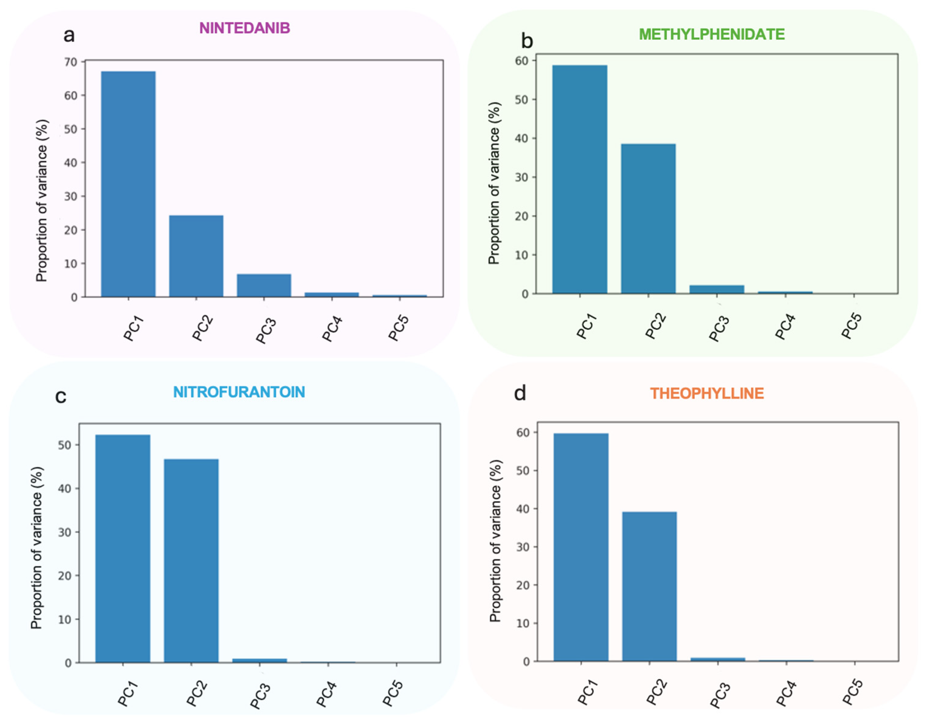
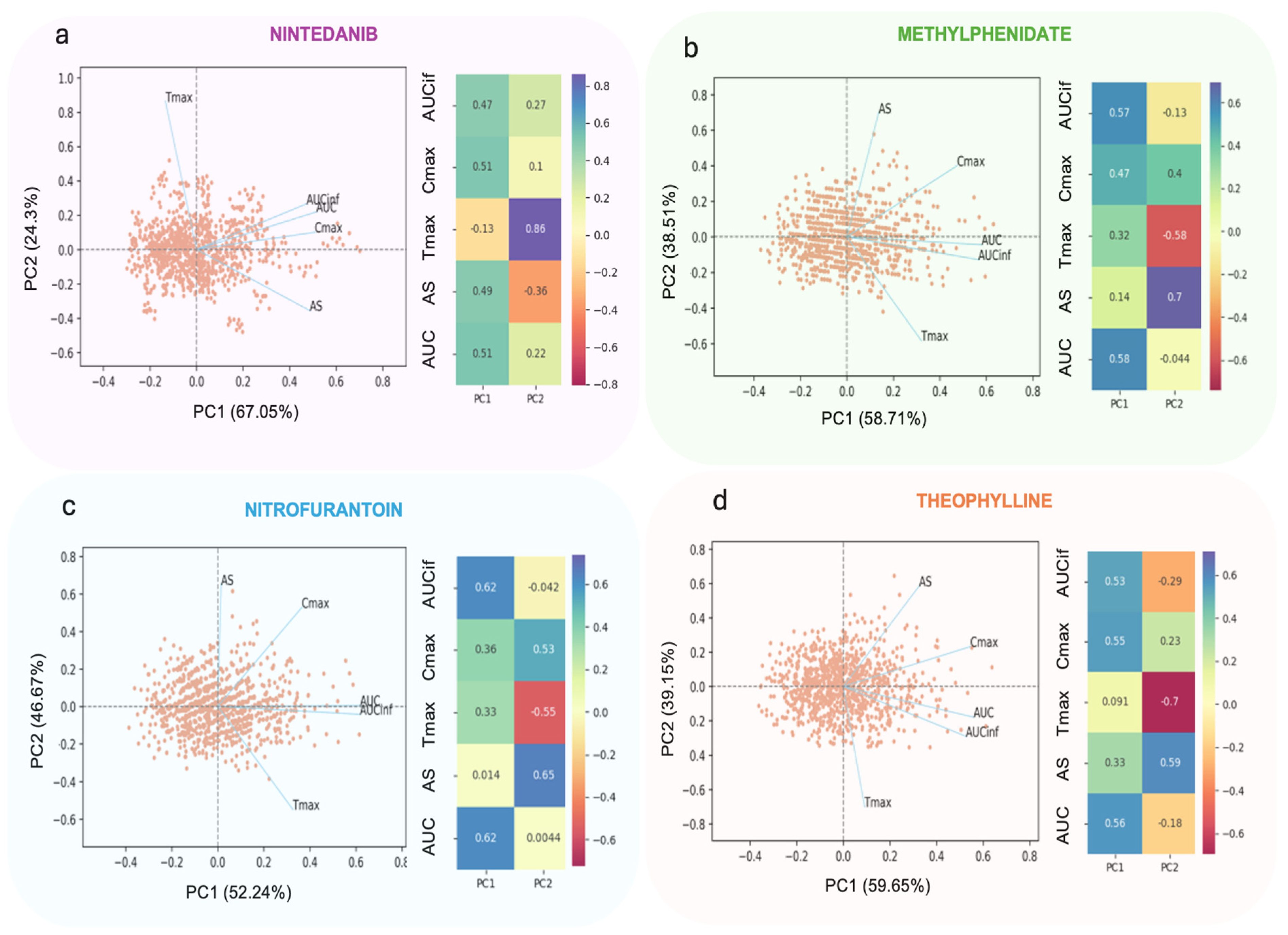
In order to find insights from each dataset and explore the interconnections between the PK parameters, PCA was utilized. The orange dots in the plane generated from the two primary PC observations represent simulated data for each of the 1000 individuals. In the meantime, the lines depict the vectors of the variables, including AS, AUC, AUCinf, Cmax, and Tmax. On the right side of each figure, the loadings of all PK parameters are displayed, where PC1 and PC2 refer to the loadings of the first and second PC, respectively. Complementary to the PCA, scree plots were constructed to identify the ideal number of PCs. The eigenvalues (representing the proportion of variance explained) are depicted on the y-axis, and the number of components is displayed on the x-axis.
Figure 1 presents the results of the PCA analysis in the case of lisdexamfetamine. It can be observed in Figure 1, specifically in the left plot, that AUC and AUCinf are closely positioned on the upper right part of the panel, adjacent to the first principal component, with similar l1 values (0.34 for AUCinf and 0.39 for AUC). Additionally, Cmax (l1 = 0.58) is positioned beside AS (l1 = 0.55), indicating a strong association between them. Tmax, currently regarded as the parameter best reflecting absorption kinetics, is situated at the upper left side of the panel. Notably, the vector representing AS is diametrically opposite to Tmax, while the two PK parameters form an angle of a little less than 180° degrees, suggesting a contrasting kinetic behavior between them.
Figure 2 illustrates the PCA results for the remaining four drugs, namely nintedanib, methylphenidate, nitrofurantoin, and theophylline. A visual inspection of Figure 2 shows that AUC and AUCinf are positioned closely together in every PCA analysis, regardless of the absorption kinetics of each drug. The Cmax in every analysis lies between AS and the pair of AUC and AUCinf, indicating a similar kinetic behavior with these PK variables. Significantly, the vector representing AS is diametrically opposite to Tmax, with the angle between them being above 90° for every PK profile. This indicates that as AS increases, reflecting faster absorption, Tmax decreases. Therefore, AS can effectively capture changes in absorption kinetics. This cannot be implied for Cmax because it forms an angle with Tmax, which is between 90°. The corresponding scree plots are depicted in Figure A1.
The high explained variance values indicate the strong descriptive capability of all the PCA models developed. Specifically, for lisdexamfetamine (Figure 1), the first and second principal components accounted for 91.97% of the total variability (49.33% and 42.64%, respectively). The total explained variability was 91.35% for nintedanib, 97.22% for methylphenidate, 98.91% for nitrofurantoin, and 98.80% for theophylline (Figure 2).

3.2.2. Random Forest

For the purposes of further investigating the correlations between the PK parameters described above using the PCA algorithm, the RF approach was used to identify the contribution of each PK parameter to Tmax. As RF is a supervised algorithm requiring the response variable in the ordinal scale before it is applied in the model, Tmax values were transformed into this scale. In this scope, Tmax was divided into quartiles, resulting in four groups. These quartiles corresponded to low, moderate, high, and very high values of Tmax.
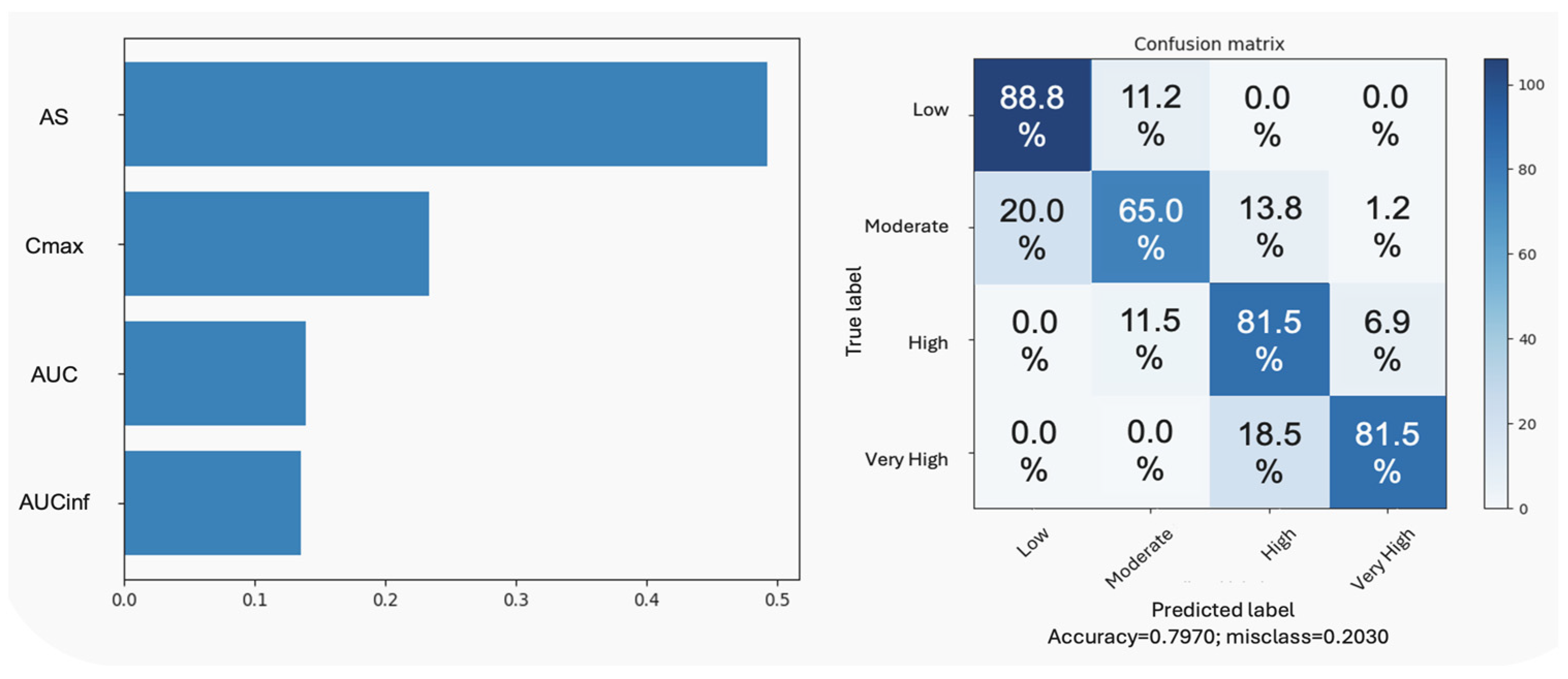
In Figure 3, the results from the RF analysis of the PK variables of lisdexamfetamine revealed that the primary contributor to Tmax was AS with a variable importance score of 49.19%, followed by Cmax, AUC, and, lastly, AUCinf. Notably, Cmax, which is commonly utilized to characterize the absorption rate, exhibited a lower contribution to Tmax with a variable importance score of 23.32%, less than half the importance score of AS. An evaluation of the confusion matrix results indicated a prediction accuracy of 79.70% for the RF model.
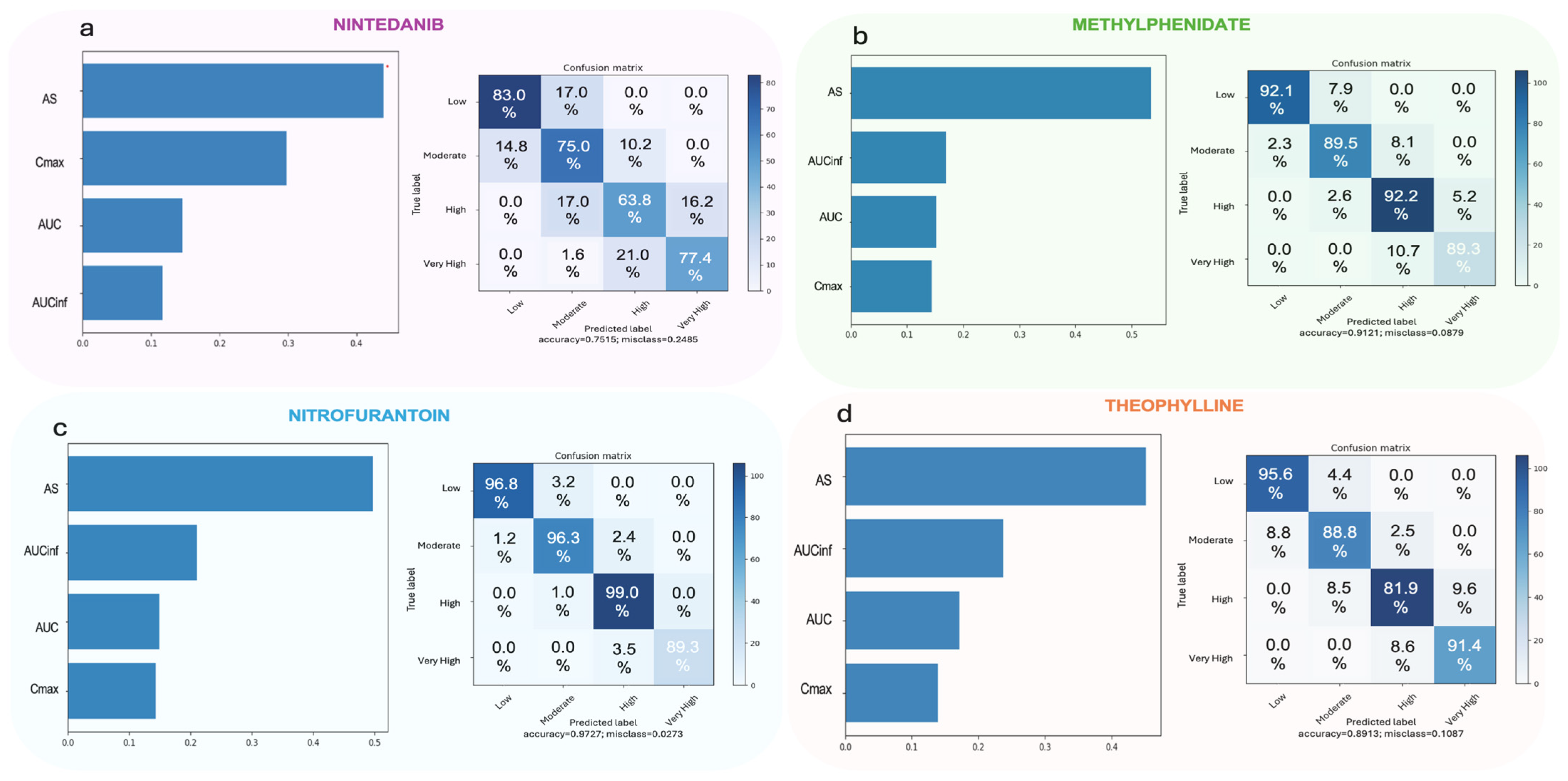
A similar analysis was performed for the other four drugs of the study (Figure 4). Notably, in Figure 4, AS contributed more to Tmax in comparison to the other PK parameters, regardless of the kinetic profile of each drug, with variable importance scores varying from 53.41% (methylphenidate) to 43.93% (nintedanib). AS was followed by either Cmax or AUCinf, suggesting that there is no distinct superior contributor to Tmax when comparing traditional PK parameters commonly used in BE studies. An evaluation of the confusion matrix results indicated a prediction accuracy of 75.15% for the RF model of nintedanib, 91.21% for methylphenidate, 97.27% for nitrofurantoin, and 89.13% for theophylline.

3.2.3. Hierarchical Clustering Analysis

The analysis continued with an unsupervised analysis and, particularly, hierarchical clustering analysis. Figure 5 shows the so-created dendrogram in the case of lisdexamfetamine, using three different types of linkage criteria, to also investigate the robustness of the clustering. These different linkage methods determine how the distance between clusters is calculated during the merging process.
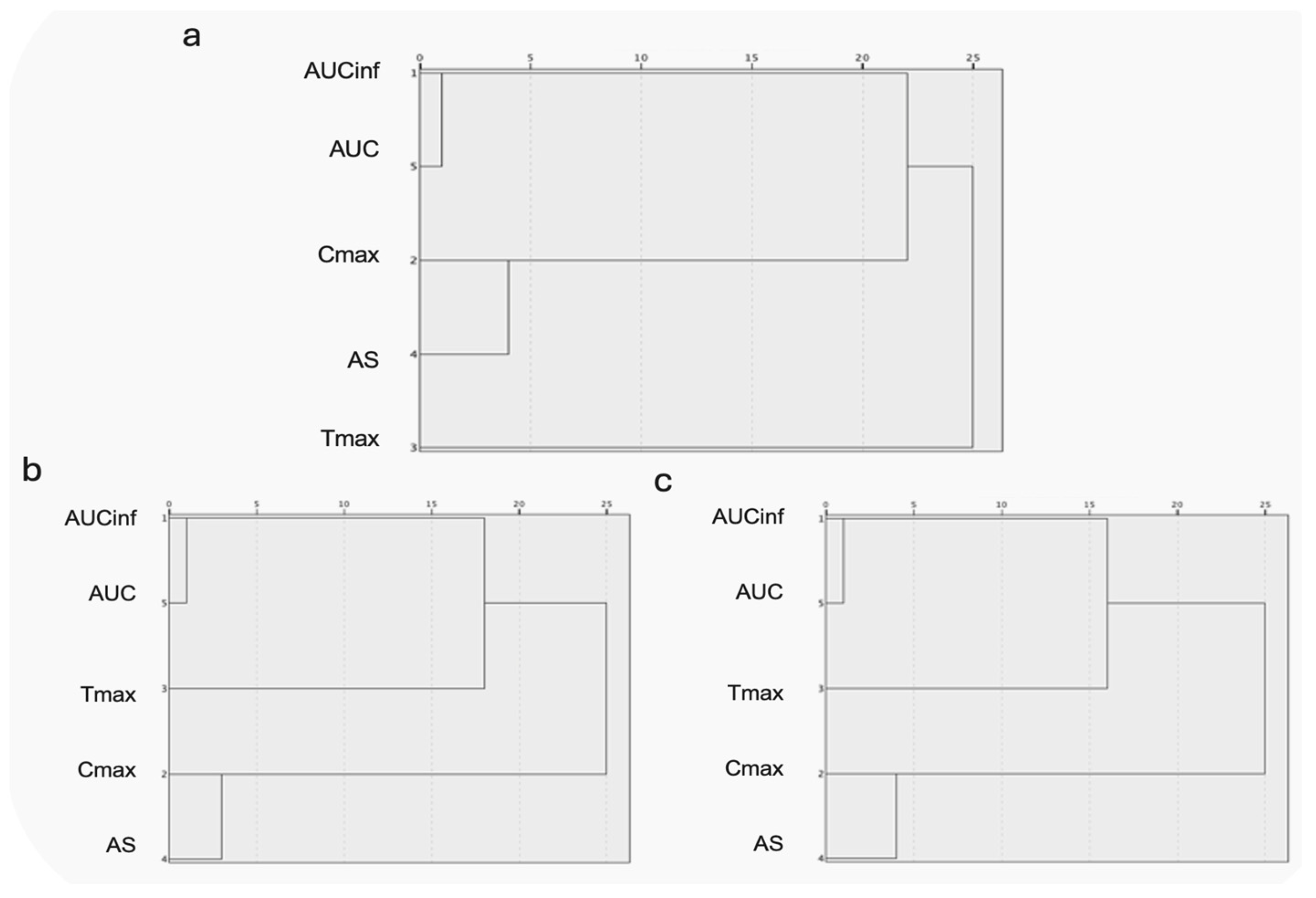
In Figure 5, it is evident that AUC and AUCinf exhibit the closest relationships, as they are the first to form a cluster regardless of the type of linkage used. Notably, AS and Cmax are the second to form a cluster in every type of linkage used, suggesting a certain similarity between them. Clustering based on average linkage between groups yields similar results to that using average linkage within groups. The primary distinction between average and single linkage is observed in the clustering of Tmax. In single linkage, Tmax is the last to form a cluster with the other PK parameters, whereas in average linkage clustering, Tmax clusters with AUC and AUCinf before clustering with Cmax and AS.
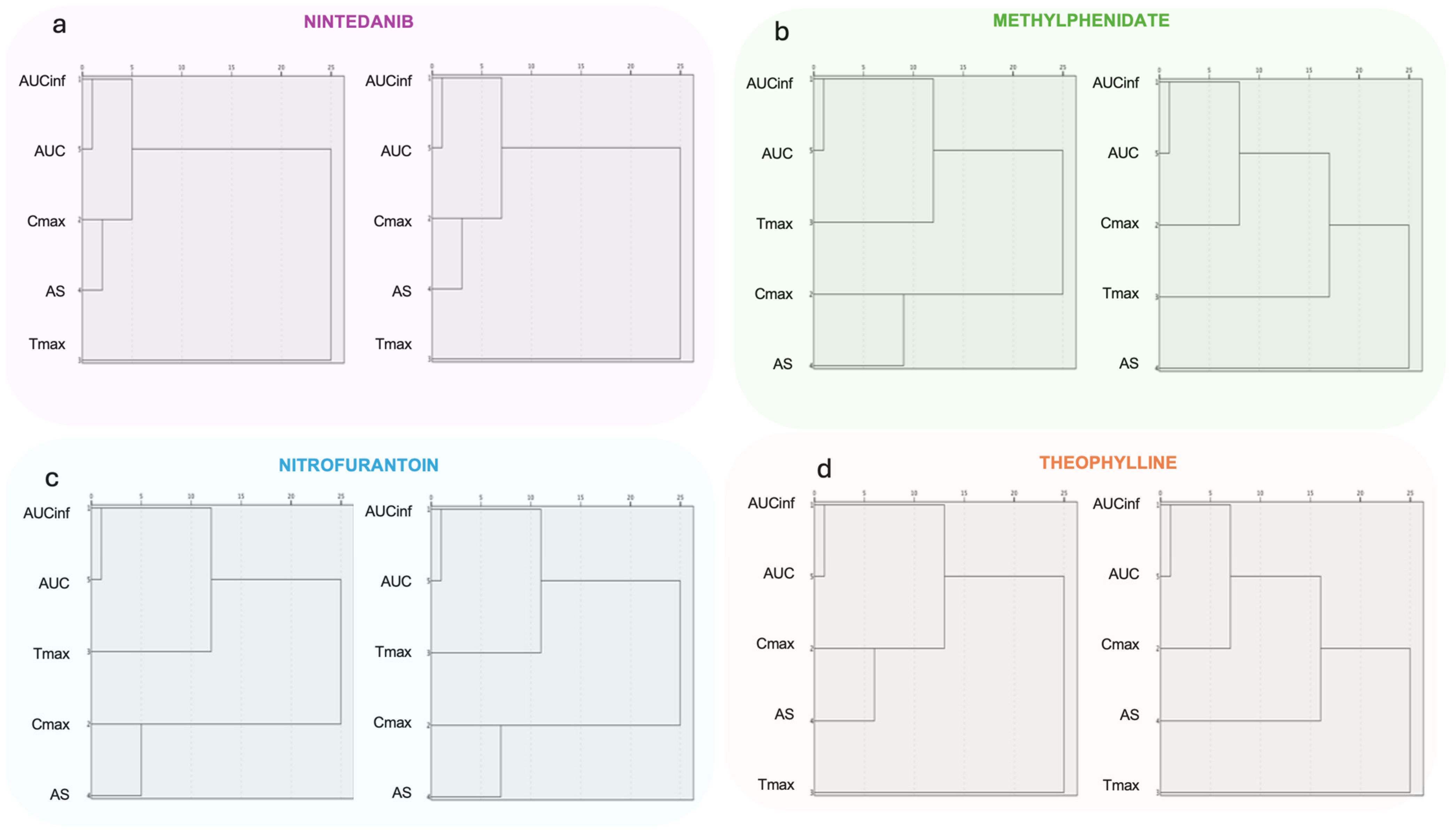
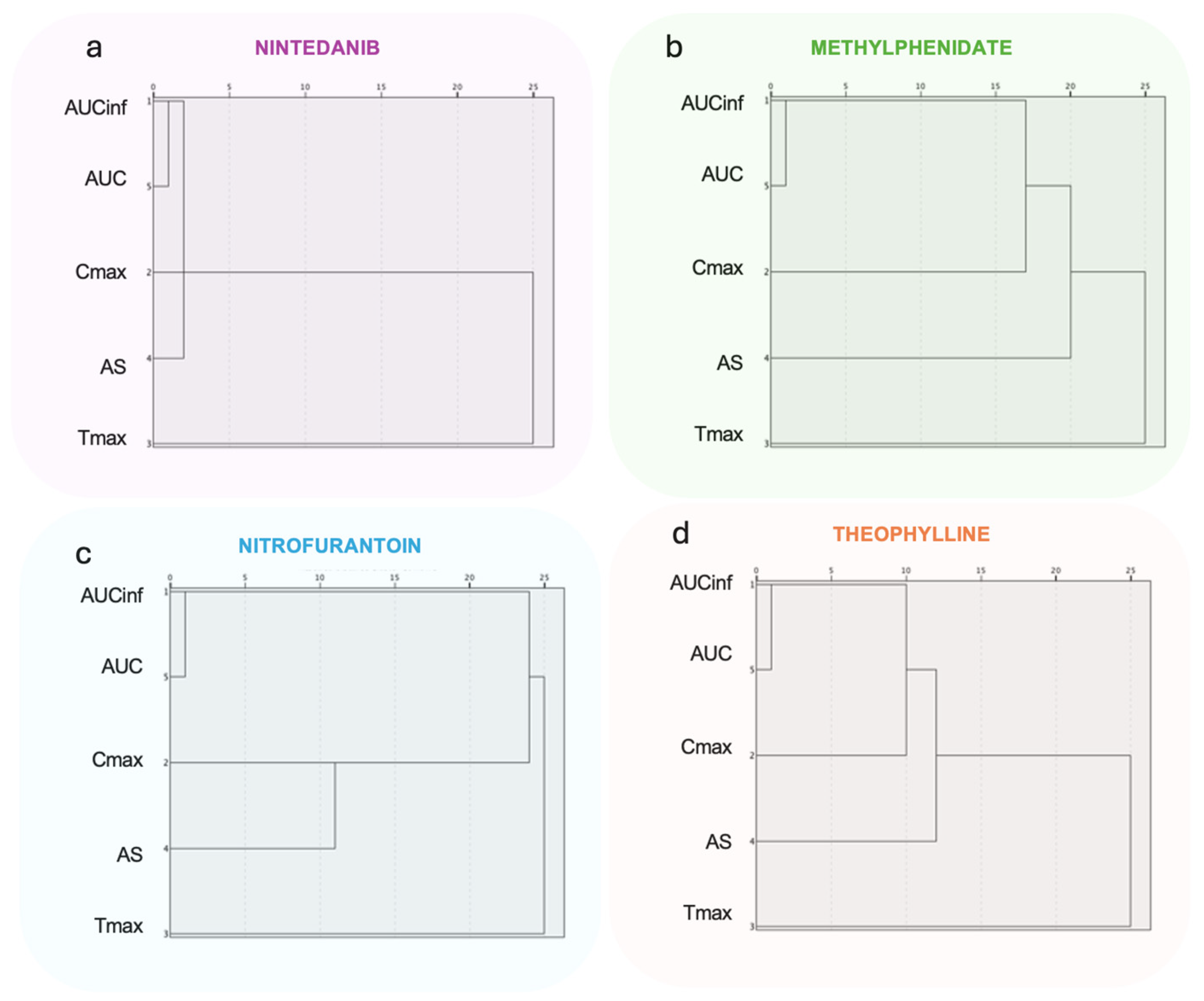
Figure 6 depicts the dendrograms for nintedanib, methylphenidate, nitrofurantoin, and theophylline. Since single linkage is the most used type of linkage, for agglomerative clustering, it was selected for the HCA analyses shown in Figure 6. Tmax, currently regarded as the parameter best reflecting absorption kinetics, is the last parameter to cluster with all the other PK parameters, suggesting a weak similarity. The clustering behavior of AS and Cmax varies depending on the absorption kinetics of each drug. Additional results with average linkage between and within groups are shown in Figure A2.

3.2.4. Artificial Neural Networks

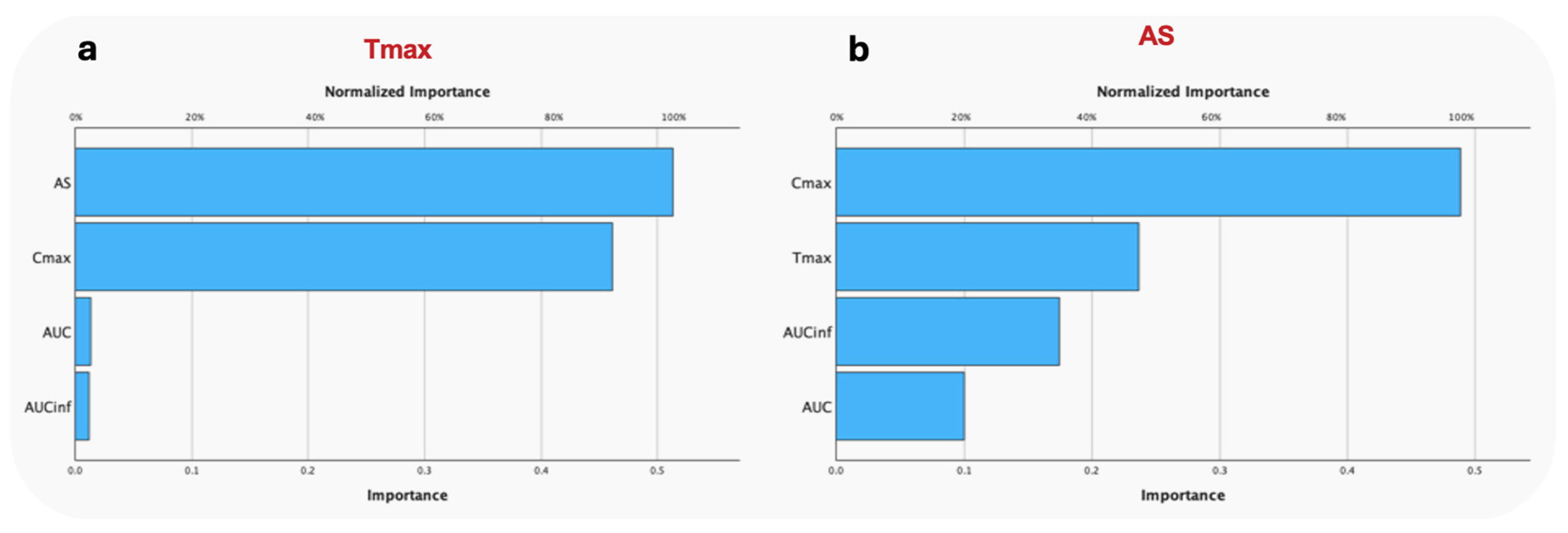
The analysis continued with the development of two ANNs where the Tmax and AS were considered as continuous response variables. Figure 7 shows the variable importance results for Tmax (Figure 7a) and AS (Figure 7b). The ANN model for Tmax exhibited a relative error of 0.002 for the training set and 0.003 for the test set. Similarly, with the ANN for AS, these relative error values were found to be 0.001 for the training set and 0.004 for the test set. These results suggest a high level of accuracy for both models.
In Figure 7a, it is obvious that AS is the most important parameter for predicting Tmax, followed closely by Cmax, which also holds significance in predicting Tmax. It is worth noting that AUC and AUCinf exhibit nearly zero importance in predicting Tmax. Meanwhile, Cmax holds more importance in predicting AS, with Tmax being the second most important parameter, having roughly half the importance of Cmax.
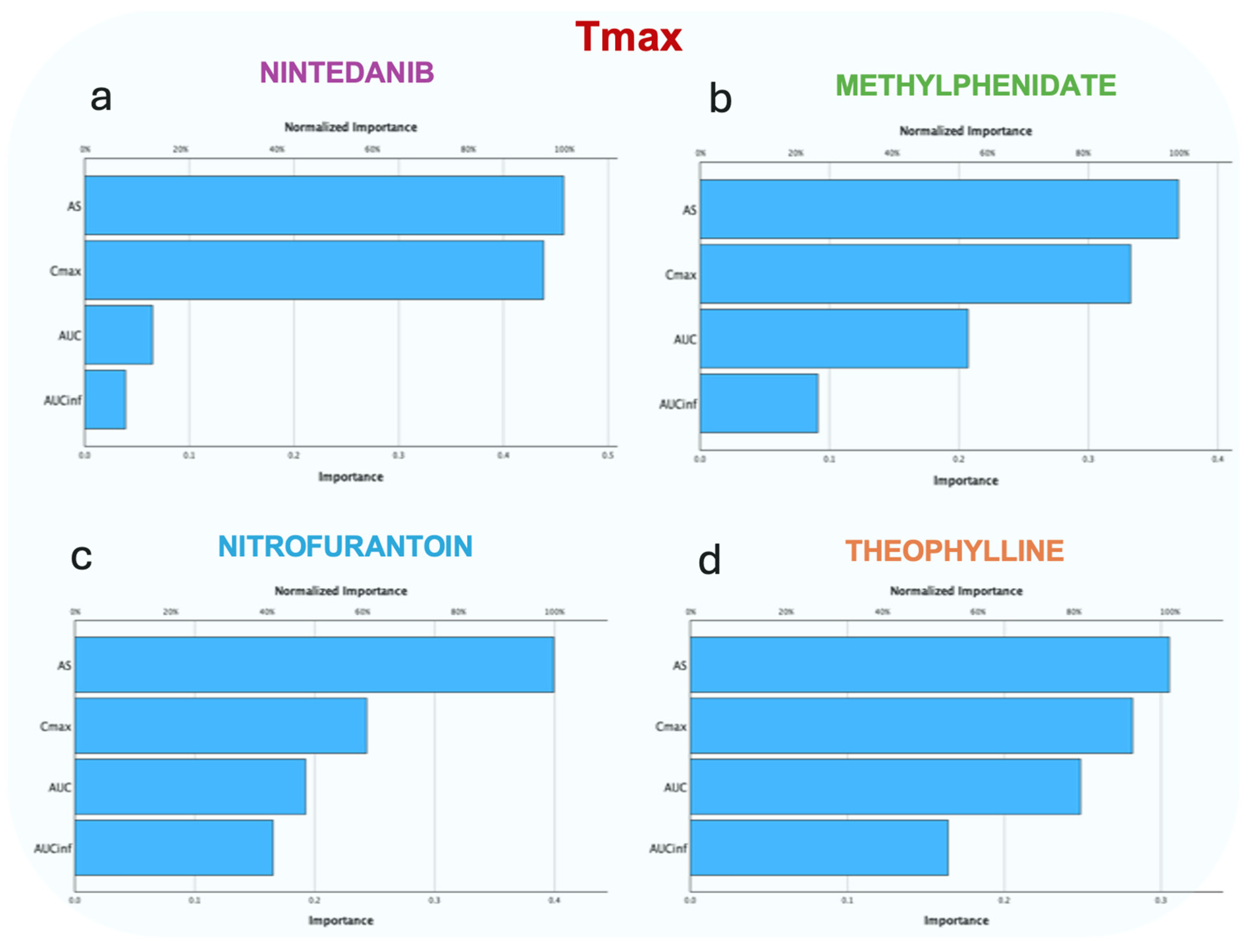
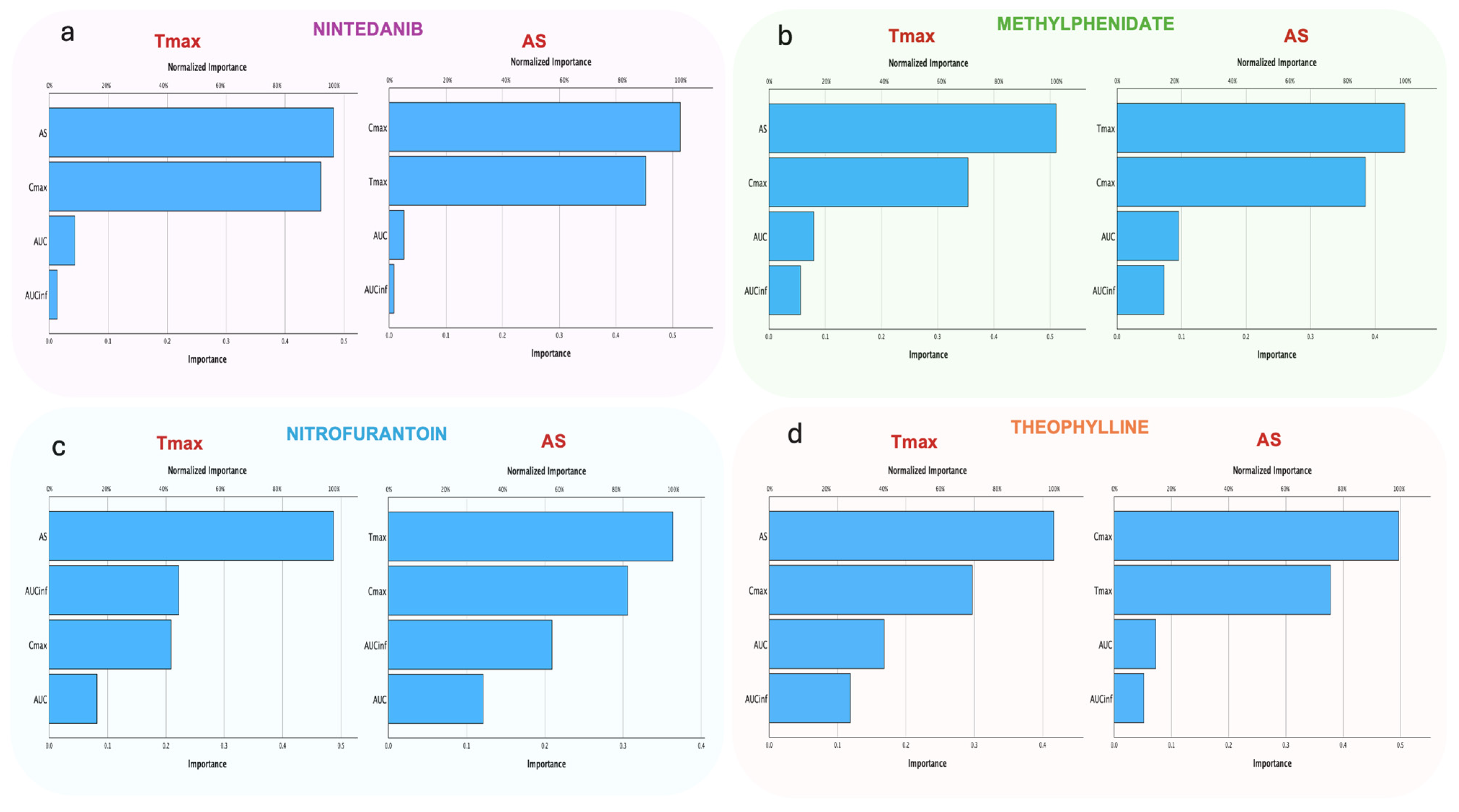
Similar ANN models (for Tmax and AS) were also built for the other four drugs of the study. For space restriction reasons, the variable importance contribution plots for the four drugs and the separate two PK parameters (AS and Tmax) are stacked together in Figure 8. Again, the ANN analyses for all drugs also demonstrated high accuracy, with relative error values for each set ranging from 0.001 to 0.039. It should be underlined that AS was the most important parameter for predicting Tmax in every analysis for each drug. On the contrary, Cmax served as the second or third important PK parameter, indicating the low relationship of Cmax with the kinetic character of Tmax.
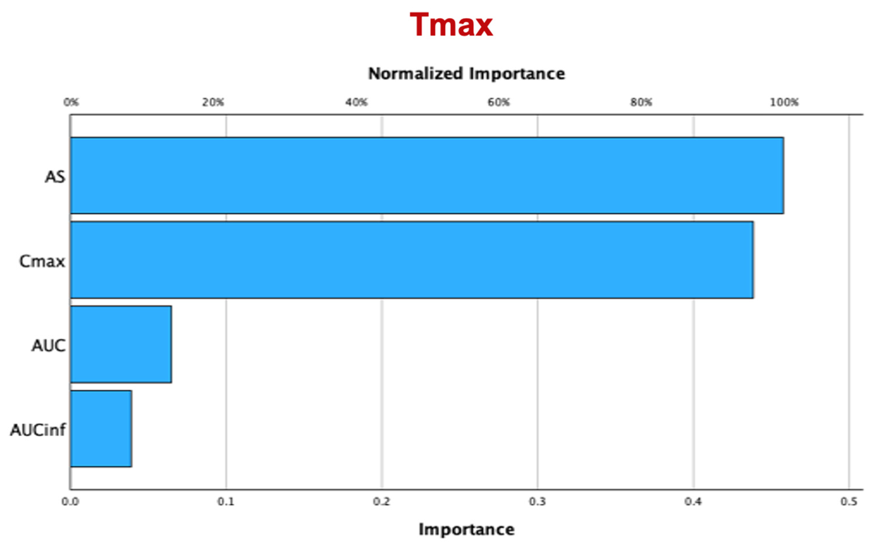
To further study the contribution of all PK parameters to Tmax, the latter was transformed into ordinal scale (see the RF analysis). A new ANN model was developed for lisdexamfetamine, and the variable contribution of the remaining parameters was estimated. Figure 9 shows the variable contribution to Tmax (when considered in the ordinal scale) in the case of lisdexamfetamine. The results are like those mentioned above when utilizing Tmax on a continuous scale. It should be underlined that AS again was found to be the most important factor for predicting Tmax, even if the latter was considered as an ordinal variable.
Additional results, when Tmax is converted to an ordinal variable, are shown in Figure A3 in the case of nintedanib, methylphenidate, nitrofurantoin, and theophylline. The primary factor to predict AS varied from drug to drug, with either Tmax followed by Cmax or Cmax followed by Tmax being the most important factors.

4. Discussion

The conventional use of Cmax as the predominant metric for the absorption rate in BE studies has faced growing scrutiny due to its significant limitations in capturing absorption kinetics [11,12,13,14,15,16,17,18]. In this study, we apply modern machine learning and deep-learning methodologies to examine and contrast the characteristics of the newly proposed metric AS with Cmax in assessing the absorption rate [19,20,21].
In pharmacokinetics, the traditional approach to explore the attributes of a PK parameter typically entails establishing its correlations with the bioavailable fraction and absorption rate constant, often assuming a specific kinetic model and using simulations. In this study, rather than relying on simple simulations, we applied ML algorithms, enabling a thorough exploration of all PK parameters concurrently. To further elaborate on the use of AS in describing the absorption rate in BE studies, the ML algorithms allowed for a comparison of AS with the traditional PK parameters and further assessment of the correlations among them. In this scope, the PK parameters of five drugs (nintedanib, methylphenidate, nitrofurantoin, lisdexamfetamine, and theophylline) with varying absorption kinetics were analyzed using three different ML algorithms (PCA, RF, and HCA) and ANNs [22,23]. To the best of our knowledge, this is the first time this novel metric has been evaluated across a range of diverse absorption kinetics while exploiting the capabilities of three different ML techniques and a deep-learning approach.
The first step of our analysis was to estimate the individual PK parameters (AS, Cmax, Tmax, AUC, and AUCinf) for the five drugs of the study. Then, the three ML approaches were applied in several ways to unveil the characteristics of AS and Cmax towards reflecting the absorption rate. The utilization of PCA, RF, HCA, and ANNs allowed for a comprehensive analysis of the relationships among the PK parameters and demonstrated the suitability of AS in effectively reflecting absorption kinetics. Each algorithm offered unique insights regarding their correlations, enhancing the robustness of our conclusions.
PCA analysis identified similarities among the PK parameters, highlighting the opposite behavior of AS to Tmax, as they are positioned in opposite directions relative to the second principal component. Significantly, the vector representing AS is diametrically opposite to Tmax. This indicates that as AS increases, reflecting faster absorption, Tmax decreases. Thus, AS effectively captures changes in absorption kinetics, unlike Cmax, which forms almost a 90-degree angle with Tmax, implying its independence from expressing the kinetic properties of absorption. RF analysis further supported the superiority of AS as an absorption rate metric. By transforming Tmax into its quartiles and using it as the response variable, RF identified AS as the primary contributor to Tmax. This finding was consistent across all drugs studied, with AS showing higher variable importance scores compared to Cmax and other PK parameters. The high prediction accuracy of the RF models underlines the reliability of AS in predicting absorption kinetics. Hierarchical clustering analyses provided additional evidence for the strong character of AS expressing kinetic properties. Finally, the ANNs models validated the findings from PCA, RF, and hierarchical clustering. The ANN models, trained on extensive PK data, demonstrated that AS was the most sensitive parameter for depicting absorption rates. The robustness of the ANN models in identifying AS as the best metric to reflect absorption kinetics unveils its potential utility in BE studies.
One point that requires special attention is the choice of drugs for the analysis. In this study, we utilized five different drugs (nintedanib, methylphenidate, nitrofurantoin, lisdexamfetamine, and theophylline) with varying pharmacokinetic properties. These different kinetic attributes are listed in Table 1. These five drugs were selected because they exhibit significantly different pharmacokinetic properties, allowing us to explore the performance of AS and Cmax under quite varying conditions. For example, we examined lisdexamfetamine, which exhibits very rapid absorption and elimination (i.e., Tmax around 1 h and the elimination of half-life in less than 1 h), as well as nintedanib, which exhibits slow absorption (Tmax can be up to 4 h) and slow elimination (the elimination of half-life ranges from 10 to 15 h). Additionally, many combinations of these performances were explored. Thus, overall, a variety of conditions have been evaluated in this work. While the use of more drugs would be beneficial, this cannot be performed in a single study. Nevertheless, it should be emphasized that the critical issue is to explore different kinetics rather than a plethora of drugs with similar kinetics. For this reason, we selected these drugs to ensure robust and reliable findings. It should also not be disregarded that these five drugs provide additional information to the initial three drugs (donepezil, hydrochloride, and amlodipine) explored in the lead paper introducing AS.
Another important aspect of the analysis is the number of subjects used in the BE studies. Officially, as required by regulatory authorities, a pivotal BE study should not include fewer than 12 subjects [1,2,3,4]. Typically, most BE studies have between 24 and 48 subjects. In our analysis, we used 1000 subjects for each drug, which is 20-to-40 times higher than usual. This was done to obtain robust estimates from the machine and deep-learning analyses, which require large sample sizes. Therefore, the sample size used (i.e., 1000) is more than adequate for our analysis and can provide reliable estimates. This is further supported by the fact that even after using five drugs with quite different pharmacokinetics and various machine and deep-learning techniques, the findings were almost identical. The latter demonstrates the desired performance of AS and its incomparable superiority over Cmax.
In this work, apart from PCA and RF, which were utilized in previous works, we further incorporated several hierarchical cluster analysis algorithms and an extensive selection of artificial neural networks (i.e., deep learning). The hierarchical cluster analysis was applied to group the data based on similarities, providing insights into the intrinsic patterns and relationships within the pharmacokinetic profiles of the drugs. This method allowed us to explore the natural grouping of the data (i.e., the PK variables) without predefined categories, thereby uncovering novel associations and trends. Additionally, we applied a variety of deep-learning techniques to our analysis. Deep learning, with its capability to model complex, non-linear relationships, enabled us to handle the complex and multifaceted nature of PK data more effectively. We utilized various architectures of neural networks, to capture several dependencies in the data. These advanced models facilitated the extraction of higher-level features from the pharmacokinetic profiles, leading to more accurate predictions. By utilizing these diverse-machine and deep-learning approaches on five drugs with distinct pharmacokinetic properties, we aimed to achieve a complete and robust analysis. The selected drugs provided a wide range of kinetic attributes, ensuring that our findings were generalizable across different scenarios. The integration of hierarchical clustering and deep-learning techniques, alongside PCA and RF, allowed us to exploit the strengths of each method, enhancing the overall reliability and depth of our study. This multifaceted approach not only validated the superior of performance of AS, compared to Cmax under varied conditions, but also demonstrated the potential of advanced analytics in pharmacokinetic research.
Despite the limitations of Cmax as a metric for the absorption rate being recognized since its early use, it has been traditionally used in BE studies for more than 40 years. In pharmacokinetics, the conventional method for examining the properties of a pharmacokinetic parameter involves identifying its relationships with the bioavailable fraction and absorption rate constant, assuming a specific type of kinetics (e.g., a one-compartment model with first-order absorption and elimination) and utilizing simple simulations. All contributions in the field of BE toward finding an appropriate metric for absorption have used pharmacokinetic modeling approaches. In the 1980s, when the foundations of this field were established, simple pharmacokinetic modeling was applied. Later, during the 2000s and 2010s, more sophisticated mechanistic models were used. However, in all these cases, there was a need to use certain pharmacokinetic models and rely on specific assumptions. In this study, we utilize modern machine-learning techniques to address an old problem from a fresh perspective. Several variations of three ML methods (PCA, RF, and hierarchical clustering) were used, as well as many types of artificial neural networks, to identify the relationships between the PK parameters. For the first time, ML algorithms are applied instead of simple simulation exercises, and all pharmacokinetic features are explored together. This is the first research work where such a variety of methods is used to unveil the relationships among the PK characteristics, and it is certainly the first time that ANNs are utilized. Each of the methods used offers different capabilities, and together they allow for the investigation of various properties of the PK characteristics (particularly AS and Cmax). The combinatorial use of all these methods allows for verifying the findings and obtaining reliable conclusions about the superiority of AS over Cmax. Finally, and perhaps most importantly, it should be emphasized that AS exhibits the ideal physical properties (i.e., units) since it is expressed in terms of concentration change over time, and its calculation does not rely on any assumptions or models. The estimation of AS can be easily conducted directly from the C-t data, even by a pocket calculator, without any assumptions.
Our findings suggest that AS is a superior metric for capturing absorption rates across various drug profiles and providing a robust alternative to Cmax in pharmacokinetics. AS not only correlates strongly with Tmax but also offers practical advantages in terms of calculation and interpretability. The ease of calculating AS, along with its appropriate units and properties, makes it a feasible metric for widespread adoption in BE studies. Also, it is important to underline that the calculation of AS does not rely on any assumptions, but it can be done through a simple non-compartmental approach. The strong (negative) correlation of AS with Tmax, suggests that it can reliably reflect the clinical outcomes associated with absorption kinetics. This correlation is crucial for ensuring that any new metric used in BE studies maintains the strict standards required for regulatory approval and therapeutic equivalence. On the contrary, Cmax exhibits properties related more to the extent of absorption, rather than the rate. In all case studies, for the five drugs with different kinetics, and the four machine-/deep-learning algorithms, AS was significantly superior to Cmax in reflecting absorption rate. These results are in line with the previous literature findings suggesting that Cmax is not an adequate metric for expressing absorption rate [10,11,12,13,14,15,16,17,18]. However, in this study we applied modern methodologies, like the three ML algorithms and ANN, allowing us to extensively explore all properties of Cmax. Moreover, it should not be disregarded that the kinetic properties of AS and its sensitivity against the absorption rate changes were shown in a previous study [21]. Finally, a quite recent study, which introduced the idea of vector-based comparisons (VBC), showed that the inflated Type II error of AS, due to its high kinetic sensitivity, can be counterbalanced [55]. Thus, the joint application of AS with the VBC approach allows for the exploration for the true absorption rate of drugs with increased statistical power. This advantage is in unambiguous contrast to current practices, where an inappropriate metric (i.e., Cmax) is used, which further exhibits low statistical power.
Overall, this study demonstrated that AS is a highly sensitive and robust metric for assessing the absorption rate of drugs. The integration of machine-/deep-learning algorithms provided a comprehensive analysis of PK parameters, consistently highlighting the superiority of AS over Cmax, under various absorption profiles. These findings suggest that AS has the potential to enhance the accuracy and reliability of BE assessments, ultimately improving therapeutic outcomes and regulatory processes. Adopting AS as a standard metric in BE studies could represent a significant advancement in the field of pharmacokinetics and bioequivalence. It is now in the hands of the regulatory agencies, like the US FDA and EMA, to consider the desired properties of AS and adopt it as the pharmacokinetic metric expressing absorption rate in bioequivalence studies.

5. Conclusions

The aim of this study was to compare the properties of AS and Cmax in expressing the absorption rate of drugs. An extensive investigation was conducted on five drugs (nintedanib, methylphenidate, nitrofurantoin, lisdexamfetamine, and theophylline) with different absorption and disposition kinetics. To maximize the exploration of AS and Cmax properties and ensure robust findings, three machine-learning algorithms (PCA, RF, and HCA), as well as artificial neural networks, were applied. This study showed that, in all drugs and methods of analysis, AS demonstrated a much superior performance in expressing an absorption rate compared to Cmax. The joint use of different techniques complemented each other and verified the findings. AS not only offers practical advantages in terms of calculation and interpretability, but, most importantly, it does not rely on any assumptions. It is calculated directly from the C-t data and exhibits the best kinetic properties compared to all other pharmacokinetic parameters. These properties ensure the reliability of AS in reflecting absorption kinetics. In turn, this facilitates the use of AS in BE studies, suggesting it can enhance the accuracy and reliability of BE assessments. The adoption of AS by regulatory authorities as an absorption-rate metric could significantly improve the accuracy and reliability of BE assessments.

Author Contributions

Conceptualization, V.D.K.; methodology, V.D.K.; software, M.K.; validation, M.K.; formal analysis, M.K.; investigation, M.K.; resources, M.K.; data curation, M.K.; writing—original draft preparation, M.K.; writing—review and editing, V.D.K.; visualization, M.K. and V.D.K.; supervision, V.D.K.; project administration, V.D.K. All authors have read and agreed to the published version of the manuscript.

Funding

This research received no external funding.

Institutional Review Board Statement

Not applicable.

Informed Consent Statement

Not applicable.

Data Availability Statement

The original contributions presented in the study are included in the article, further inquiries can be directed to the corresponding author.

Conflicts of Interest

The authors declare no conflict of interest.

Appendix A

Figure A1. Scree plots to define the number of principal components (PC) for the PCA models for (a) nintedanib, (b) methylphenidate, (c) nitrofurantoin, and (d) theophylline.
Applsci 14 06115 g0a1
Figure A2. Hierarchical clustering (dendrograms) of the pharmacokinetic variables of (a) nintedanib, (b) methylphenidate, (c) nitrofurantoin, and (d) theophylline. Each panel shows the results after using average linkage between groups (left graph) and within groups (right graph).
Applsci 14 06115 g0a2
Figure A3. Variable importance scores for the artificial neural network models developed for the remaining four drugs of the study when Tmax was considered the response variable. The panels correspond to the models for (a) nintedanib, (b) methylphenidate, (c) nitrofurantoin, and (d) theophylline. In all cases, Tmax was measured on an ordinal scale.
Applsci 14 06115 g0a3

References

  1. European Medicines Agency; Committee for Medicinal Products for Human Use (CHMP). Guideline on the Investigation of Bioequivalence; London, UK, 20 January 2010. Available online: https://www.ema.europa.eu/en/documents/scientific-guideline/guideline-investigation-bioequivalence-rev1_en.pdf (accessed on 12 June 2024).
  2. Food and Drug Administration Center for Drug Evaluation and Research (CDER). Guidance for Industry Bioavailability and Bioequivalence Studies Submitted in NDAs or INDs—General Considerations. 2014. Available online: https://www.fda.gov/media/88254/download (accessed on 12 June 2024).
  3. Niazi, S. Handbook of Bioequivalence Testing (Drugs and the Pharmaceutical Sciences), 2nd ed.; Taylor & Francis Group: Boca Raton, FL, USA, 2014. [Google Scholar]
  4. Karalis, V. Modeling and Simulation in Bioequivalence. In Modeling in Biopharmaceutics, Pharmacokinetics and Pharmacodynamics. Homogeneous and Heterogeneous Approaches; Springer International Publishing: Cham, Switzerland, 2016; pp. 227–255. [Google Scholar]
  5. Bois, F.Y.; Tozer, T.N.; Hauck, W.W.; Chen, M.-L.; Patnaik, R.; Williams, R.L. Bioequivalence: Performance of Several Measures of Extent of Absorption. Pharm. Res. 1994, 11, 715–722. [Google Scholar] [CrossRef] [PubMed]
  6. Reppas, C.; Lacey, L.F.; Keene, O.N.; Macheras, P.; Bye, A. Evaluation of Different Metrics as Indirect Measures of Rate of Drug Absorption from Extended Release Dosage Forms at Steady-State. Pharm. Res. 1995, 12, 103–107. [Google Scholar] [CrossRef] [PubMed]
  7. Chen, M.-L.; Lesko, L.; Williams, R.L. Measures of Exposure versus Measures of Rate and Extent of Absorption. Clin. Pharmacokinet. 2001, 40, 565–572. [Google Scholar] [CrossRef] [PubMed]
  8. Jackson, A.J. Determination of in Vivo Bioequivalence. Pharm. Res. 2002, 19, 227–228. [Google Scholar] [CrossRef] [PubMed]
  9. Endrenyi, L.; Tothfalusi, L. Metrics for the Evaluation of Bioequivalence of Modified-Release Formulations. AAPS J. 2012, 14, 813–819. [Google Scholar] [CrossRef] [PubMed]
  10. Stier, E.M.; Davit, B.M.; Chandaroy, P.; Chen, M.-L.; Fourie-Zirkelbach, J.; Jackson, A.; Kim, S.; Lionberger, R.; Mehta, M.; Uppoor, R.S.; et al. Use of Partial Area under the Curve Metrics to Assess Bioequivalence of Methylphenidate Multiphasic Modified Release Formulations. AAPS J. 2012, 14, 925–926. [Google Scholar] [CrossRef] [PubMed]
  11. Rostami-Hodjegan, A.; Jackson, P.R.; Tucker, G.T. Sensitivity of Indirect Metrics for Assessing “Rate” in Bioequivalence Studies—Moving the “Goalposts” or Changing the “Game”. J. Pharm. Sci. 1994, 83, 1554–1557. [Google Scholar] [CrossRef] [PubMed]
  12. Basson, R.P.; Cerimele, B.J.; DeSante, K.A.; Howey, D.C. Tmax: An Unconfounded Metric for Rate of Absorption in Single Dose Bioequivalence Studies. Pharm. Res. 1996, 13, 324–328. [Google Scholar] [CrossRef] [PubMed]
  13. Chen, M.-L. An Alternative Approach for Assessment of Rate of Absorption in Bioequivalence Studies. Pharm. Res. 1992, 9, 1380–1385. [Google Scholar] [CrossRef]
  14. Lacey, L.F.; Keene, O.N.; Duquesnoy, C.; Bye, A. Evaluation of Different Indirect Measures of Rate of Drug Absorption in Comparative Pharmacokinetic Studies. J. Pharm. Sci. 1994, 83, 212–215. [Google Scholar] [CrossRef]
  15. Endrenyi, L.; Al-Shaikh, P. Sensitive and Specific Determination of the Equivalence of Absorption Rates. Pharm. Res. 1995, 12, 1856–1864. [Google Scholar] [CrossRef] [PubMed]
  16. Schall, R.; Luus, H.G.; Steinijans, V.W.; Hauschke, D. Choice of Characteristics and Their Bioequivalence Ranges for the Comparison of Absorption Rates of Immediate-Release Drug Formulations. Int. J. Clin. Pharmacol. Ther. 1994, 32, 323–328. [Google Scholar] [PubMed]
  17. Tothfalusi, L.; Endrenyi, L. Without Extrapolation, Cmax/AUC Is an Effective Metric in Investigations of Bioequivalence. Pharm. Res. 1995, 12, 937–942. [Google Scholar] [CrossRef] [PubMed]
  18. Vincze, I.; Endrényi, L.; Tóthfalusi, L. Bioequivalence Metrics for Absorption Rates: Linearity, Specificity, Sensitivity. Acta Pharm. Hung. 2019, 89, 17–21. [Google Scholar] [CrossRef]
  19. Karalis, V.D. On the Interplay between Machine Learning, Population Pharmacokinetics, and Bioequivalence to Introduce Average Slope as a New Measure for Absorption Rate. Appl. Sci. 2023, 13, 2257. [Google Scholar] [CrossRef]
  20. Karalis, V.D. Machine Learning in Bioequivalence: Towards Identifying an Appropriate Measure of Absorption Rate. Appl. Sci. 2022, 13, 418. [Google Scholar] [CrossRef]
  21. Karalis, V.D. An in Silico Approach toward the Appropriate Absorption Rate Metric in Bioequivalence. Pharmaceuticals 2023, 16, 725. [Google Scholar] [CrossRef]
  22. Shamout, F.G.; Zhu, T.; Clifton, D.A. Machine Learning for Clinical Outcome Prediction. IEEE Rev. Biomed. Eng. 2021, 14, 116–126. [Google Scholar] [CrossRef]
  23. James, G.; Hastie, T.; Tibshirani, R.; Witten, D. An Introduction to Statistical Learning with Applications in R; Springer: Berlin/Heidelberg, Germany, 2017. [Google Scholar]
  24. Schlender, J.-F.; Meyer, M.; Thelen, K.; Krauss, M.; Willmann, S.; Eissing, T.; Jaehde, U. Development of a Whole-Body Physiologically Based Pharmacokinetic Approach to Assess the Pharmacokinetics of Drugs in Elderly Individuals. Clin. Pharmacokinet. 2016, 55, 1573–1589. [Google Scholar] [CrossRef] [PubMed]
  25. Watanabe-Uchida, M.; Narukawa, M. Utilization of Population Pharmacokinetics in Drug Development and Provision of the Results to Healthcare Professionals. Int. J. Clin. Pharmacol. Ther. 2017, 55, 25–31. [Google Scholar] [CrossRef]
  26. Wang, W.-J.; Bansal, A.; Bennette, C.S.; Basu, A. Mimicking Clinical Trials Using Real-World Data: A Novel Method and Applications. Med. Decis. Making 2023, 43, 275–287. [Google Scholar] [CrossRef]
  27. Zhang, F.; Jia, R.; Gao, H.; Wu, X.; Liu, B.; Wang, H. In Silico Modeling and Simulation to Guide Bioequivalence Testing for Oral Drugs in a Virtual Population. Clin. Pharmacokinet. 2021, 60, 1373–1385. [Google Scholar] [CrossRef]
  28. European Medicines Agency, Committee for Medicinal Products for Human Use (CHMP). Assessment Report; Of eu International Non-Proprietary Name: Nintedanib. 2014. Available online: https://www.ema.europa.eu/en/medicines/human/EPAR/ofev (accessed on 12 June 2024).
  29. Marzin, K.; Kretschmar, G.; Luedtke, D.; Kraemer, S.; Kuelzer, R.; Schlenker-Herceg, R.; Schmid, U.; Schnell, D.; Dallinger, C. Pharmacokinetics of Nintedanib in Subjects with Hepatic Impairment. J. Clin. Pharmacol. 2018, 58, 357–363. [Google Scholar] [CrossRef]
  30. Schmid, U.; Doege, C.; Dallinger, C.; Freiwald, M. Population Pharmacokinetics of Nintedanib in Patients with Idiopathic Pulmonary Fibrosis. Pulm. Pharmacol. Ther. 2018, 48, 136–143. [Google Scholar] [CrossRef]
  31. Wind, S.; Schmid, U.; Freiwald, M.; Marzin, K.; Lotz, R.; Ebner, T.; Stopfer, P.; Dallinger, C. Clinical Pharmacokinetics and Pharmacodynamics of Nintedanib. Clin. Pharmacokinet. 2019, 58, 1131–1147. [Google Scholar] [CrossRef]
  32. Adjei, A.; Teuscher, N.S.; Kupper, R.J.; Chang, W.-W.; Greenhill, L.; Newcorn, J.H.; Connor, D.F.; Wigal, S. Single-Dose Pharmacokinetics of Methylphenidate Extended-Release Multiple Layer Beads Administered as Intact Capsule or Sprinkles versus Methylphenidate Immediate-Release Tablets (Ritalin®) in Healthy Adult Volunteers. J. Child Adolesc. Psychopharmacol. 2014, 24, 570–578. [Google Scholar] [CrossRef]
  33. Geneesmiddeleninformatiebank. Public Assessment Report; Medikinet 5/10/20 Mg; Tabletten Medikinet Retard 10/20/30/40 Mg Methylphenidate Hydrochloride. 2006. Available online: https://www.geneesmiddeleninformatiebank.nl/pars/h34030.pdf (accessed on 12 June 2024).
  34. Gutiérrez-Casares, J.R.; Quintero, J.; Segú-Vergés, C.; Rodríguez Monterde, P.; Pozo-Rubio, T.; Coma, M.; Montoto, C. In Silico Clinical Trial Evaluating Lisdexamfetamine’s and Methylphenidate’s Mechanism of Action Computational Models in an Attention-Deficit/Hyperactivity Disorder Virtual Patients’ Population. Front. Psychiatry 2023, 14, 939650. [Google Scholar] [CrossRef]
  35. Teuscher, N.; Adjei, A.; Findling, R.; Greenhill, L.; Kupper, R.; Wigal, S. Population Pharmacokinetics of Methylphenidate Hydrochloride Extended-Release Multiple-Layer Beads in Pediatric Subjects with Attention Deficit Hyperactivity Disorder. Drug Des. Devel. Ther. 2015, 9, 2767. [Google Scholar] [CrossRef]
  36. Lyauk, Y.K.; Stage, C.; Bergmann, T.K.; Ferrero-Milliani, L.; Bjerre, D.; Thomsen, R.; Dalhoff, K.P.; Rasmussen, H.B.; Jürgens, G. Population Pharmacokinetics of Methylphenidate in Healthy Adults Emphasizing Novel and Known Effects of Several Carboxylesterase 1 (CES1) Variants. Clin. Transl. Sci. 2016, 9, 337–345. [Google Scholar] [CrossRef]
  37. Wijma, R.A.; Huttner, A.; Koch, B.C.P.; Mouton, J.W.; Muller, A.E. Review of the Pharmacokinetic Properties of Nitrofurantoin and Nitroxoline. J. Antimicrob. Chemother. 2018, 73, 2916–2926. [Google Scholar] [CrossRef]
  38. College ter beoordeling van geneesmiddelen. Public Assessment Report; Scientific Discussion; Nitrofurantoïne 50 Mg and 100 Mg Focus Care, Hard Capsules (Nitrofurantoin as Macrocrystals). 2022. Available online: www.geneesmiddeleninformatiebank.nl/pars/h127575.pdf. (accessed on 12 June 2024).
  39. Sharma, R.P.; Burgers, E.J.; Beltman, J.B. Development of a Physiologically Based Pharmacokinetic Model for Nitrofurantoin in Rabbits, Rats, and Humans. Pharmaceutics 2023, 15, 2199. [Google Scholar] [CrossRef]
  40. Food and Drug Administration. CLINICAL REVIEW 2208510; Lisdexamfetamine Dimesylate (Vyvanase) Chewable Tablets. 2009. Available online: https://www.fda.gov/files/drugs/published/208510-Vyvanse-clinical-prea.pdf (accessed on 12 June 2024).
  41. Läkemedelsverket. Public Assessment Report; Scientific Discussion Elvanse (Lisdexamfetamine Dimesylate); SE/H/1839/01-03. 2019. Available online: https://docetp.mpa.se/LMF/Elvansecapsule,hardENGPAR_09001bee80cde265.pdf (accessed on 12 June 2024).
  42. AUSPAR. Australian Public Assessment Report for Lisdexamfetamine Dimesilate. 2013. Available online: https://www.tga.gov.au/sites/default/files/auspar-lisdexamfetamine-dimesilate-131023.pdf (accessed on 12 June 2024).
  43. Comiran, E.; Carlos, G.; Barreto, F.; Pechanksy, F.; Fröehlich, P.E.; Limberger, R.P. Lisdexamfetamine and Amphetamine Pharmacokinetics in Oral Fluid, Plasma, and Urine after Controlled Oral Administration of Lisdexamfetamine. Biopharm. Drug Dispos. 2021, 42, 3–11. [Google Scholar] [CrossRef]
  44. Ermer, J.; Corcoran, M.; Lasseter, K.; Martin, P.T. Relative Bioavailabilities of Lisdexamfetamine Dimesylate and D-Amphetamine in Healthy Adults in an Open-Label, Randomized, Crossover Study after Mixing Lisdexamfetamine Dimesylate with Food or Drink. Ther. Drug Monit. 2016, 38, 769–776. [Google Scholar] [CrossRef]
  45. Dolder, P.C.; Strajhar, P.; Vizeli, P.; Hammann, F.; Odermatt, A.; Liechti, M.E. Pharmacokinetics and Pharmacodynamics of Lisdexamfetamine Compared with D-Amphetamine in Healthy Subjects. Front. Pharmacol. 2017, 8, 617. [Google Scholar] [CrossRef]
  46. Ma, Y.; Xue, L.; Chen, X.; Kang, Y.; Wang, Y.; Wang, L. Population Pharmacokinetics of Theophylline in Adult Chinese Patients with Asthma and Chronic Obstructive Pulmonary Disease. Int. J. Clin. Pharm. 2018, 40, 1010–1018. [Google Scholar] [CrossRef]
  47. Australian Industrial Chemicals Introduction Scheme. 1H-Purine-2,6-Dione, 3,7-Dihydro-1,3dimethyl (Theophylline) Evaluation Statement. 2022. Available online: https://www.industrialchemicals.gov.au/sites/default/files/2022-06/EVA00032%20-%20Evaluation%20statement%20-%2030%20June%202022.pdf (accessed on 12 June 2024).
  48. OECD. THEOPHILLINE CAS N°: 58-55-9. 2001. Available online: https://hpvchemicals.oecd.org/UI/handler.axd?id=f9abfd36-c689-46e5-92da-ff5e7a672e00 (accessed on 12 June 2024).
  49. Zhang, Z.; Castelló, A. Principal Components Analysis in Clinical Studies. Ann. Transl. Med. 2017, 5, 351. [Google Scholar] [CrossRef]
  50. Yu, W.; Gu, Y.; Li, Y. Efficient Randomized Algorithms for the Fixed-Precision Low-Rank Matrix Approximation. SIAM J. Matrix Anal. Appl. 2018, 39, 1339–1359. [Google Scholar] [CrossRef]
  51. Wallace, M.L.; Mentch, L.; Wheeler, B.J.; Tapia, A.L.; Richards, M.; Zhou, S.; Yi, L.; Redline, S.; Buysse, D.J. Use and Misuse of Random Forest Variable Importance Metrics in Medicine: Demonstrations through Incident Stroke Prediction. BMC Med. Res. Methodol. 2023, 23, 1–12. [Google Scholar] [CrossRef]
  52. Zhang, Z.; Murtagh, F.; Van Poucke, S.; Lin, S.; Lan, P. Hierarchical Cluster Analysis in Clinical Research with Heterogeneous Study Population: Highlighting Its Visualization with R. Ann. Transl. Med. 2017, 5, 75. [Google Scholar] [CrossRef]
  53. Schmidhuber, J. Deep Learning in Neural Networks: An Overview. Neural Netw. 2015, 61, 85–117. [Google Scholar] [CrossRef]
  54. Abut, S.; Okut, H.; Zackula, R.; James Kallail, K. Deep Neural Networks and Applications in Medical Research. In Artificial Intelligence; IntechOpen: London, UK, 2023. [Google Scholar]
  55. Karalis, V. A Vector Theory of Assessing Clinical Trials: An Application to Bioequivalence. J. Cardiovasc. Dev. Dis. 2024, 11, 185. [Google Scholar] [CrossRef]
Figure 1. Principal component analysis of the pharmacokinetic parameters of lisdexamfetamine. Left illustration: biplot of the two principal components with the individual scores (orange dots) and the loadings (blue lines) of the pharmacokinetic parameters. Central illustration: scree plot to identify the number of principal components. Right illustration: loading values for the two initial principal components.
Applsci 14 06115 g001
Figure 2. Four different principal component analyses were conducted, each referring to one of the additional four drugs in the study. Each plot corresponds to (a) nintedanib, (b) methylphenidate, (c) nitrofurantoin, and (d) theophylline. Left panel of each set: biplot of the two principal components showing the individual scores (orange dots) and the loadings (blue lines) of the pharmacokinetic parameters. Right panel of each set: loading values for the two initial principal components.
Applsci 14 06115 g002
Figure 3. A random forest classifier model when Tmax (in ordinal scale) was used as the response variable for lisdexamfetamine. The left panel shows the variable importance scores, while the right panel displays the confusion matrix.
Applsci 14 06115 g003
Figure 4. Four different random forest classifier models, when Tmax (in ordinal scale) was used as the response variable, each one referring to the additional four drugs in the study. Each panel corresponds to (a) nintedanib, (b) methylphenidate, (c) nitrofurantoin, and (d) theophylline. In each panel, the left graph shows the variable importance scores, while the right graph displays the confusion matrix.
Applsci 14 06115 g004
Figure 5. Hierarchical clustering (dendrograms) of the pharmacokinetic variables of lisdexamfetamine. Each plot shows the different types of linkage used: (a) single linkage, (b) average linkage between groups, and (c) average linkage within groups.
Applsci 14 06115 g005
Figure 6. Hierarchical clustering of the pharmacokinetic variables of the four remaining drugs using single linkage. Each plot shows the dendrogram for (a) nintedanib, (b) methylphenidate, (c) nitrofurantoin, and (d) theophylline.
Applsci 14 06115 g006
Figure 7. Variable importance scores for two artificial neural network models developed for lisdexamfetamine. The plots show the contribution of the pharmacokinetic parameters to Tmax (a) and AS (b). Both Tmax and AS were measured on a numerical scale.
Applsci 14 06115 g007
Figure 8. Variable importance scores for the artificial neural network models developed for the remaining four drugs of the study. The panels correspond to the models for (a) nintedanib, (b) methylphenidate, (c) nitrofurantoin, and (d) theophylline. The left part of each panel shows the contribution of the pharmacokinetic parameters to Tmax, while the right shows the contribution to AS (both measured on a numerical scale).
Applsci 14 06115 g008
Figure 9. Variable importance scores for the artificial neural network models developed for lisdexamfetamine, when Tmax is measured on an ordinal scale.
Applsci 14 06115 g009
Table 1. Pharmacokinetic characteristics and sampling points for each drug based on literature. As indicated by the Tmax and t1/2 values, a variety of drugs with diverse kinetic properties were selected for the analysis.
Medicine NameTmax (h)t1/2 (h)Sampling Points (h)References
Nintedanib2–410–150, 0.5, 1, 1.5, 2, 2.5, 3, 3.5, 4, 4.5, 5, 6, 7, 8, 10, 12, 24[28,29,30,31]
Methylphenidate1–22–30, 0.5, 1, 1.5, 2, 2.5, 3, 4, 4.5, 5, 5.5, 6, 6.5, 7, 8, 8.5, 9, 9.5, 10, 10.5, 12, 15, 19, 24[32,33,34,35,36]
Nitrofurantoin2–40.5–1.30, 0.5, 1, 1.5, 2, 2.33, 2.67, 3, 3.33, 3.67, 4, 4.5, 5, 6, 8, 12, 24[37,38,39]
Lisdexamfetamine1<10, 0.5, 0.75, 1, 1.5, 2, 2.5, 3, 4, 6, 9, 12, 16, 24[40,41,42,43,44,45]
Theophylline1–2 3–90, 0.33, 0.67, 1, 1.25, 1.55, 1.75, 2, 2.25, 2.50, 2.75, 3, 4, 6, 8, 10, 12, 16, 24, 48, 72[46,47,48]
Key: Tmax, the time at which the peak plasma concentration of the drug is observed (after an immediate-release formulation in the fasting state); t1/2, elimination half-life.
Disclaimer/Publisher’s Note: The statements, opinions and data contained in all publications are solely those of the individual author(s) and contributor(s) and not of MDPI and/or the editor(s). MDPI and/or the editor(s) disclaim responsibility for any injury to people or property resulting from any ideas, methods, instructions or products referred to in the content.