Feature-Model-Based In-Process Measurement of Machining Precision Using Computer Vision

Abstract

In-process measurement of machining precision is of great importance to advanced manufacturing, which is an essential technology to realize compensation machining. In terms of cost-effectiveness and repeatability of computer vision, it has become a trend to replace traditional manual measurement with computer vision measurement. In this paper, an in-process measurement method is proposed to improve precision and reduce the costs of machining precision. Firstly, a universal features model framework of machining parts is established to analyze the CAD model and give standard information on the machining features. Secondly, a window generator is proposed to adaptively crop the image of the machining part according to the size of features. Then, the automatic detection of the edges of machining features is performed based on regions of interest (ROIs) from the cropped image. Finally, the measurement of machining precision is realized through a Hough transform on the detected edges. To verify the effectiveness of the proposed method, a series of in-process measurement experiments were carried out on machined parts with various features and sheet metal parts, such as dimensional accuracy measurement tests, straightness measurement tests, and roundness measurement tests under the same part conditions. The best measurement accuracy of this method for dimensional accuracy, straightness, and roundness were 99%, 97%, and 96%, respectively. In comparison, precision measurement experiments were conducted under the same conditions using the Canny edge detection algorithm, the sub-pixel edge detection algorithm, and the Otsu–Canny edge detection algorithm. Experimental results show that the feature-model-based in-process measurement of machining precision using computer vision demonstrates superiority and effectiveness among various measurement methods.

1. Introduction

Intelligent manufacturing is characterized by autonomy and self-optimization, which requires as few people as possible to participate in decision-making in the manufacturing process [1]. A digital workshop, known as the minimum implementation unit for intelligent manufacturing, is a combination of a group of machine tools that perform a specific processing sequence of products [2]. The measurement of the machining precision of the workpiece is necessary for forming a closed-loop control in a digital workshop.

Commonly used measurement methods of machining precision include off-line measurement and on-line measurement [3]. Off-line measurement requires moving the workpiece outside the production line. In this method, additional errors such as clamp error, spindle/slide motion errors, thermal deformations, and vibration are inevitable, making it difficult to ensure measurement accuracy. In contrast, on-line measurement can be carried out when the workpiece is on the production line. Under this condition, if the measurement can be carried out in the process of the machining operation, it is referred to as in-process measurement. High efficiency is required for in-process measurement, to ensure that the measurement process is completed in the time interval from one cutting operation to the next. This is necessary for achieving compensation machining by matching the compensation results with the CAD model. Among various measurement methods, contact measurement is widely used for its stability and anti-interference capability. However, it is often difficult to mount a contact measuring instrument on machine tools. Thus, non-contact measurement is receiving increasing attention due to its advantages, such as wide measurement range, fast measurement speed, and low cost. Commonly used non-contact measurement techniques include LiDAR [4], machine vision technology [5], etc. Machine vision technology [6] is widely used in sorting, positioning, feature recognition, size measurement, and other aspects of industrial products. Compared with traditional laser measurement, machine vision technology has the advantages of lower cost, better stability, and higher measurement efficiency [7].

Machine-vision-based position measurement has the characteristics of non-contact, high accuracy, and high stability [8], and has very important applications in areas such as vehicles [9,10], aerospace [11,12], robots [13], and industrial production [14,15]. Automated industrial inspection relies on computer vision technology to achieve highly efficient and safe production [16]. The application of machine vision detection technology is expanding from simple measurement of the size of automotive gaskets [17] to more complex evaluation of the plane size of mechanical components [18] and is undergoing further development to include distance measurement [19] and visual monitoring of the rolling process [20]. The countersink detection method proposed by Mohammed Salah further improves the detection speed during the machining process [21]. Many studies have shown that the continuous evolution of machine vision technology has successfully achieved on-line detection of industrial measurement technology [22,23,24]. Precision measurement plays a crucial role in ensuring machining quality. Jiang, BC proposed a high-precision bearing size measurement method using unidirectional matrices and partial domain effects [25]. Bin Li achieves part contour extraction through wavelet denoising and Canny edge detection. [26]. Compared to traditional manual measurement methods, these machine-vision-based measurement technologies have significant advantages in eliminating human bias and improving measurement speed [17,22].

The precise measurement of part dimensions is challenging due to various interference factors present in the manufacturing process, including machining marks, metal cutting, and dust. These interference factors decrease the machine vision measurement accuracy in the studies cited above. To address this issue, a feature-model-based in-process measurement of machining precision using computer vision is proposed in this paper. The key to this method is that regions of interest (ROIs) containing target features can be automatically selected using a features model, which improves the accuracy of the algorithm because many noise sources such as processing traces are filtered out. Additionally, the computational efficiency can be greatly reduced since all the pixels except in the ROIs are eliminated from the data to be calculated. To achieve this goal, we propose an improved Canny edge detection algorithm that focuses on edge feature detection of ROIs.

The remainder of this paper is organized as follows. Section 2 provides a detailed introduction to the principle of feature-model-based in-process measurement of machining precision using computer vision. To demonstrate the effectiveness of the proposed method, Section 3 conducted experimental validation and analysis of the measurement results. Finally, Section 4 provides some useful conclusions.

2. Measurement Algorithm

This paper achieves precise measurement of part size parameters in images by establishing a model of machining features and using an improved Canny edge detection algorithm. First, a template image is generated with variable dimensions based on the part’s blueprint. Then, the part image is preprocessed, including steps such as noise removal and feature enhancement, to ensure that the machining feature model can accurately match the part image. Next, the area requiring precise detection is delineated. Finally, the improved Canny edge detection algorithm is used to extract the edge information of the parts, and the Hough transform is used to further obtain the part size data, completing the area detection and measurement of the part. The schematic diagram of the proposed method is shown in Figure 1.

2.1. Image Preprocessing

2.1.1. Image Interpolation

Bilinear interpolation is a commonly used image interpolation method for calculating new pixel values between discrete pixel values [27]. This method is based on the principle of linear interpolation and performs calculations in both the horizontal and the vertical directions. The focus of the bilinear interpolation algorithm is to design a gradient template for determining the precise position of each pixel in the image, followed by polynomial interpolation to calculate new pixel coordinates. For the image I to be interpolated, the size and pixel position of the target image must be determined. For each target pixel, the four closest original image pixels are found. As shown in Figure 2, these are the pixels in the top left, top right, bottom left, and bottom right. The coordinates of these four pixels are assumed to be (x₁, y₁), (x₂, y₁), (x₁, y₂), and (x₂, y₂), respectively, where x₁ and x₂ are the nearest neighbors in the horizontal direction, and y₁ and y₂ are the nearest neighbors in the vertical direction. The specific process is as follows:

First, a linear interpolation in the horizontal direction is performed. Next, the distance ratio of the target pixel to the nearest neighboring pixels in the horizontal direction is calculated. Then, based on the pixel values of Q₁₁ = (x₁, y₁) and Q₂₁ = (x₂, y₁), the pixel value of the temporary pixel R₁ = (x, y₁) is calculated. Finally, based on the pixel values of Q₁₂ = (x₁, y₂) and Q₂₂ = (x₂, y₂), the pixel value of the temporary pixel R₂ = (x, y₂) is calculated. R₂ represents the position of the target pixel relative to the nearest neighboring pixels in the horizontal direction. The following formula

$$f(R_1)=\frac{x_2-x}{x_2-x_1}f(Q_{11})+\frac{x-x_1}{x_2-x_1}f(Q_{21})$$

(1)

similarly, is used to calculate R₂ = (x, y₂).

Then, linear interpolation is performed in the vertical direction, calculating the distance ratio of the target pixel to the nearest neighboring pixels in that direction. According to the pixel values of R₁ = (x, y₁) and R₂ = (x, y₂), the final result P = (x, y) pixel value is calculated as:

$$f(P)=\frac{y_2-y}{y_2-y_1}f(R_1)+\frac{y-y_1}{y_2-y_1}f(R_2)$$

(2)

The bilinear interpolation method considers the weights of the nearest four pixels, which better preserves the image’s smoothness and details.

2.1.2. Weighted Median Filter

Compared to traditional median filter methods, weighted median filtering considers the weights of the pixels when calculating the image’s median filter, resulting in a smoother outcome. Weighted median filters have certain advantages in image processing [28]. They can retain the edge information of the parts and have a good removal effect on different types of noise. The principle can be summarized as follows:

First, for a given pixel in the image, a 3 × 3 window is used to determine its neighborhood size. The size of the neighborhood directly affects the smoothing effect, and larger neighborhoods can achieve better smoothing results. However, if the neighborhood is too large, this can lead to blurred loss of edge information, making the output image blurred. Secondly, pixels within the neighborhood are sorted by brightness values to obtain an ordered sequence. Then, Formula (3) is used to calculate the weight of each pixel, utilizing the distance from the center pixel as the weight. The weighted median function can be expressed as:

$${\mathrm{Med}}_w(I_{\mathrm{in}}(x,y))=media{n}_{i,j}\{I_{\mathrm{in}}(x+i,y+j)\cdot w(i,j)\}$$

(3)

where I_in(x, y) is the pixel value of the input image at position (x, y), I_out(x, y) is the pixel value of the output image at position (x, y), and Med_w is the weighted median function, which calculates the weighted median of the pixel values in the input neighborhood.

Finally, the weighted median is calculated based on pixel weights, using the median as the new value for that pixel. The weighted median is used as the output pixel value. The pixel formula processed can be expressed as:

$$I_{\mathrm{out}}(x,y)={\mathrm{Med}}_w(I_{\mathrm{in}}(x,y))$$

(4)

where i and j are the coordinate offsets of pixels in the neighborhood, and w(i, j) is the weight of the corresponding pixel.

2.2. Establishing a Machining Feature Model for Design

To effectively measure the machining of parts, it is necessary to construct a machining feature model for subsequent image matching. First, the part blueprint created by Computer-Aided Design (version: AutoCAD 2014) software or third-party tools is obtained. Drawings of parts are usually created directly in CAD software or imported through third-party tools. Subsequently, CAD standard data will be converted to DXF format, and each component of the input drawing will be analyzed, such as circles, lines, arcs, etc. As shown in Figure 3, this can capture relevant dimension information, such as radius size, starting point position, center position, and arc degree of the arc, as well as starting and ending point positions of lines. Then, the parsed parameter information will be integrated into a standardized data structure to keep data consistency. For each graphic element, the process generates a series of point sets based on its parameter information. The generated sets of points represent the position and shape of these transformed sets of points and feature points in a unified reference coordinate system. Taking a circle as an example, a series of points are generated based on the circle’s center and radius that accurately represent the position of the circumference. Finally, according to the pixel standards of industrial cameras, the size of the machining feature model is adjusted to ensure dimensional consistency from the part drawing to the actual machining process. The specific conversion between arcs and line segments is as follows:

2.2.1. Parsing the Set of Points Generated by Straight Lines

When drawing a straight line on paper, it is necessary to determine the starting point (x₁, y₁) and the ending point (x₂, y₂). Then, the two points are connected together to form a straight line. First, a computer screen is composed of discrete pixels with each white block representing a pixel. Therefore, it is necessary to determine which pixels need to be smeared to simulate the line. In this study, the distance d between two points is calculated and then a straight line on the pixel can be obtained through linear interpolation. The specific distance obtained is as follows:

$$d=\sqrt{{(x_2-x_1)}^2+{(y_2-y_1)}^2}$$

(5)

Next, the number of generated points numPoints is calculated:

$$numPoints=\frac{d}{gridsize}$$

(6)

Then, linear interpolation is used to generate the pixel coordinates of each point on the line segment in the image:

$$x_i=x_1+\frac{i}{numPo\mathrm{int}s}\times (x_2-x_1)$$

(7)

$$y_i=y_1+\frac{i}{numPo\mathrm{int}s}\times (y_2-y_1)$$

(8)

2.2.2. Parsing the Point Set Generated by Arcs

Similar to the process of drawing a straight line, the circle of a part is drawn by the radius size, starting point position, center position, and degree of arc. First, the coordinates of the starting point (x_s, y_s) and the center of the circle (x_o, y_o). are clarified. Then, the arctangent function is used to obtain the starting angle θ of the arc.

$${\theta }_i=ata{n}_2(y_s-y_o,x_s-x_o)$$

(9)

The starting angle must be adjusted according to the position of the starting point to ensure that it is in the correct quadrant. The coordinates (x_i, y_i) of each point on the arc are determined by the following Formula (10):

$$x_i=x_o+R\cdot cos({\theta }_i)·gridsize$$

(10)

$$y_i=y_o+R\cdot sin({\theta }_i)·gridsize$$

(11)

where gridsize is the actual length represented by each pixel, obtained from the proportional relationship between the actual depth dh and the camera.

2.3. Matching of Machining Feature Model with Part Drawing

The matching of the processing feature model with the part image is crucial for the subsequent ROI extraction and part recognition. However, the processing feature models are typically represented as line segments in white pixels, and they lack the surface characteristics, while the actual part images in the background may contain various colors and patterns, making it difficult to directly match the processing feature model with the part image. To solve this problem, it is necessary to fill the processing feature model to enhance the contrast with the background, thereby facilitating the subsequent matching and ROI extraction. The first step in the filling process is to expand the processing feature model. The black pixels adjacent to the white pixels are converted to white pixels, thereby expanding the white regions in the image. An n × n window is set to slide on the image of the machining feature model, and if the area covered by the window contains white pixels, the pixel at the center of the window is set to white. Through the expansion operation, the small holes and narrow gaps in the processing feature model are filled, making it a continuous and distinct white region.

Next, an erosion operation is performed on the expanded processing feature model, causing white areas to contract inward. The erosion operation uses an n × n window that slides across the image. This eliminates small objects, isolated points, and spikes in the image, while also smoothing the boundaries of larger objects. Since the dilation operation filled the edges of the model, the erosion operation will not remove these connected regions, as shown in Figure 4.

The matching of the fabrication feature model and the part image is based on centroids. First, the centroid of the part image is calculated by taking the weighted average of the positions of all the points in the image. Secondly, the Euclidean distance between the centroid of the fabrication feature model and the centroid of the part image is calculated to determine the offset between the two. Then, based on the calculated centroid offset, a translation operation is performed on the fabrication feature model to align its centroid with the centroid of the part image. This aligns the two images on the same plane. Finally, rotation-invariant features are introduced, and the fabrication feature model is rotated counterclockwise around the centroid to begin matching overlapping pixels between the model and the part image. During rotation, the set of overlapping points between the fabrication feature model and the part image is calculated to find the optimal matching position between the model image and the part image. Because the fabrication feature model is an ideal representation, while the part image has noise and machining marks as interfering factors, the overlay of the images cannot be a complete match. Therefore, when the matching rate reaches 90% or higher, the ROI can be selected based on the dimensional elements within the model. The position relationship between the fabrication feature model and the part image is used to determine the ROI. The ROI contains the features to be measured, and the location and size information of the original ROI image is determined. The range of the ROI in the image is calculated based on the width d of the part ROI. For example, in Figure 5, the ROI range can be determined based on the dimensional information of the fabrication feature model. The ROI boundaries or rectangular area are adaptively determined based on the size of the part, with the specific formula being as follows.

$$d=\frac{w}{h}\left(l\times gridsize\right)$$

(12)

where w and h are the length and width of the photo, respectively, and l is the design length of the part.

If the ROI width increases, it will cover a larger image area and may include more background information, but will also increase the impact of background noise. If the ROI width d decreases, the ROI will only include a smaller region around the part, which can reduce the impact of background noise, but may result in a lack of contextual information. Therefore, based on the requirements of the part in this article and the impact of width changes on the results, the most appropriate ROI width d should be selected for evaluation. Algorithm 1 lists the pseudocode for analyzing CAD 2D drawings to obtain machining feature models, and then matching to obtain the ROI.

Algorithm 1: Feature-Model-based ROI Construction

Input: CAD 2D drawing, part image I

Output: ROI image

1. Begin 2. convert CAD drawings to DXF format. 3. read the information of elements from the DXF format file 4. for i = the number of elements 5.   if Current element = line 6.     obtain the coordinates of the arc L(x, y) according to Formulas (7) and (8) 7.   else If Current element = arc 8.     obtain the coordinates of the straight line R(x, y) according      to Formulas (10) and (11) 9.   end 10. end 11. add coordinates L or R to the machining feature model Im 12. match Im with I → ROI image

2.4. ROI-Based Canny Edge Detection

After determining the ROI range based on the procedure described in the previous section, the next step is to perform a quantitative analysis of the edge detection function within the ROI. First, based on the edge features, the Gaussian first-order derivative model is selected. Then, the frequency domain characteristics of the model are analyzed to determine the optimal filter parameters. Finally, the expression of the edge detection operator is derived. This ensures that the optimal edge detection function is obtained in the continuous domain. Afterward, the function that meets the design criteria is sampled and finally mapped to the ROI to obtain the Canny operator. The implementation steps are described below.

2.4.1. Gaussian Filtering for Smoothing Images

Before performing edge detection, the noise in the ROI of the image usually needs to be smoothed. The Gaussian filter is a linear filter obtained by normalizing the two-dimensional Gaussian function after sampling. The formula is in the form of the two-dimensional Gaussian function used by the Gaussian filter in the Canny operator:

$$G(x,y)=\frac{1}{2\pi {\sigma }^2}{e}^{\left(-\frac{x^2+y^2}{2{\sigma }^2}\right)}$$

(13)

where G(x, y) is the value of the Gaussian function at the coordinate point (x, y), and σ (sigma) is the standard deviation of a Gaussian function, which determines the width and smoothness of the function.

2.4.2. Gradient Calculation of ROI Pixels

To calculate the gradient magnitude and direction of each pixel in the ROI image I, first-order partial derivatives are used. The gradient operator used is the Sobel operator, which calculates the gradient magnitude and direction based on the Sobel operator to find the gradients of the image. First, the convolution template is applied separately in the x and y directions, and then the gradient magnitude and direction are computed.

The formulas are as follows:

$$G_x=\left[\begin{array}{ccc}-1& 0& +1\\ -2& 0& +2\\ -1& 0& +1\end{array}\right]\times I$$

(14)

$$G_y=\left[\begin{array}{ccc}-1& -2& -1\\ 0& 0& 0\\ +1& +2& +1\end{array}\right]\times I$$

(15)

where I is the grayscale image matrix, represented by

$$G_{xy}(i,j)=\sqrt{G_x{(i,j)}^2+G_y{(i,j)}^2}$$

(16)

The gradient intensity matrix G_xy is calculated.

2.4.3. Non-Maximum Suppression and Dual Threshold Processing

Due to the convolution of filters sliding over the image within a window, lower gradient values, G_p1 and G_p2, appear on either side of the actual edge center. For detected edge pixel G_p, the pixel gradient strength is compared with adjacent pixels along the positive gradient direction G_p1 and negative gradient direction G_p2. If this is the maximum value, this indicates that the pixel is at the edge center and is retained; otherwise, the pixel value is set to zero. By setting high and low thresholds, the gradient magnitude image categorizes pixels into three types: strong edge, weak edge, and non-edge. The high threshold determines strong edges, the low threshold determines non-edges, and weak edges require further analysis to determine if they are actual edges. The spatial connectivity of weak edges is analyzed to determine true edges. Components connected spatially to strong and weak edges are considered true edges, while unconnected components are excluded. Finally, weak edge pixels are connected to strong edge pixels based on paths connected to form complete edges. Algorithm 2 lists pseudocode based on the steps of the improved Canny edge detection algorithm.

Algorithm 2: Improved Canny Edge Detection
	Input: Part image I, ROI image IROI
	Output: Edge image Iout
1. Begin 2. I ← to compute Formulas (2) and (4) for I 3. for i = IROI(x) 4.  for j = IROI(y) 5.  IG(x, y) ←to compute Formula (13) for I. 6.   Gp ← to compute Formula (16) for I G(x, y). 7.   if Gp ≥ Gp1 and Gp ≥ Gp2 8.    Gp may be an edge 9.   else 10.   Gp should be suppressed 11.   end 12.   if Gp ≥ HighThreshold, 13.  Gp is a strong edge 14.   else if Gp > LowThreshold 15.    Gp is a weak edge 16.   else 17.   Gp should be suppressed 18.   end 19.   if Gp = LowThreshold and Gp connected to a strong edge pixel 20.   Gp is a strong edge 21.   else 22.   Gp should be suppressed 23.   end 24.  Iout(x,y) = Gp 25.  end 26. end

2.5. Actual Machining Feature Extraction

After completing the improved Canny edge detection based on ROIs, the Hough transform can be used for further analysis of detected edges to extract linear and circular features in the image. The Hough transform is a commonly used technique in image processing and computer vision for detecting line or curve features. It was originally proposed by Paul Hough in 1962. The Hough transform uses a transformation between two coordinate spaces, mapping curves or lines with the same shape in one space to points in another coordinate space to form peaks, thus transforming the problem of detecting arbitrary shapes into a problem of detecting statistical peaks. Here is the pseudocode for obtaining the ROI:

2.5.1. Hough Transform line Feature Detection

The straight line passing through points (x, y) can be represented in Cartesian coordinates as:

$$y=kx+b$$

(17)

where k is the slope of the line, and b is the intercept. The parameters of all lines passing through two points A (x₀, y₀) and B (x₁, y₁) satisfy Formula (16), which determines a family of lines. Formula (16) can be rewritten as:

$$b=-kx+y$$

(18)

Points A and B can be regarded as a straight line in the parameter plane of Figure 6b, where −x is the slope of the line, y is the intercept, and k and b are variables, as shown in Figure 6. Points in the image space correspond one by one to the lines in the parameter space. In Figure 6, it can be seen that the lines corresponding to point A and point B in the image space intersect at a point in the parameter space, which is the line determined by AB and corresponds to a unique point in the parameter space. The coordinate values (b₀, k₀) of this point are also the parameters of line AB.

However, in practical applications, the parameter space cannot choose a Cartesian coordinate system because the special line x = c (perpendicular to the x-axis, with an infinite slope and a constant c) in the Cartesian coordinate space of the original image cannot be represented in the parameter space based on the Cartesian coordinate system. To avoid the inability to recognize parallel lines, polar coordinates are used as parameter space, and Formula (18) is replaced by a straight-line polar coordinate equation:

$$r=x\cos \theta +y\sin \theta$$

(19)

where r is the distance from the line to the coordinate origin, and θ is the angle between the horizontal direction and the perpendicular of the detection line. The representation in the polar coordinate system is shown in Figure 7, and the Hough transform can be determined based on the intersection point of two sine curves r₁ and r₂ in polar coordinates.

2.5.2. Hough Transform Circle Feature Detection

Its detection approach is the same as Hough line detection, but it is different from the fitting of lines. In the Hough transform, the fitting of a circle requires three parameters, namely (x, y, r), where x and y represent coordinates and r represents the radius of the circle. The parameters are determined according to the following formula:

$${(x-a)}^2+{(y-b)}^2=r^2$$

(20)

where (a, b) is the center of the circle, and r is the radius.

As shown in Figure 8a, if the two-dimensional points (x, y) are fixed, the parameters can be found according to Formula (23). The parameter space will be three-dimensional (a, b, R). All parameters that satisfy (x, y) will be located on the surface of the cone at the vertex (x, y, 0). In 3D space, arc parameters can be identified by the intersection points of many conical surfaces, which are defined by points in 2D arcs. This process can be divided into two stages. The first step is to fix the radius, and then find the optimal center in the two-dimensional parameter space. The second step is to find the optimal radius in the one-dimensional parameter space. Figure 8b shows the point-to-point dual diagram of the Hough circle detection algorithm.

Finally, the distance between the center of the circle and the line is calculated to obtain the required measurement information. Additional measurement information is obtained by calculating the position of the circle based on the detected radius and center.

3. Measurement Implementation and Verification

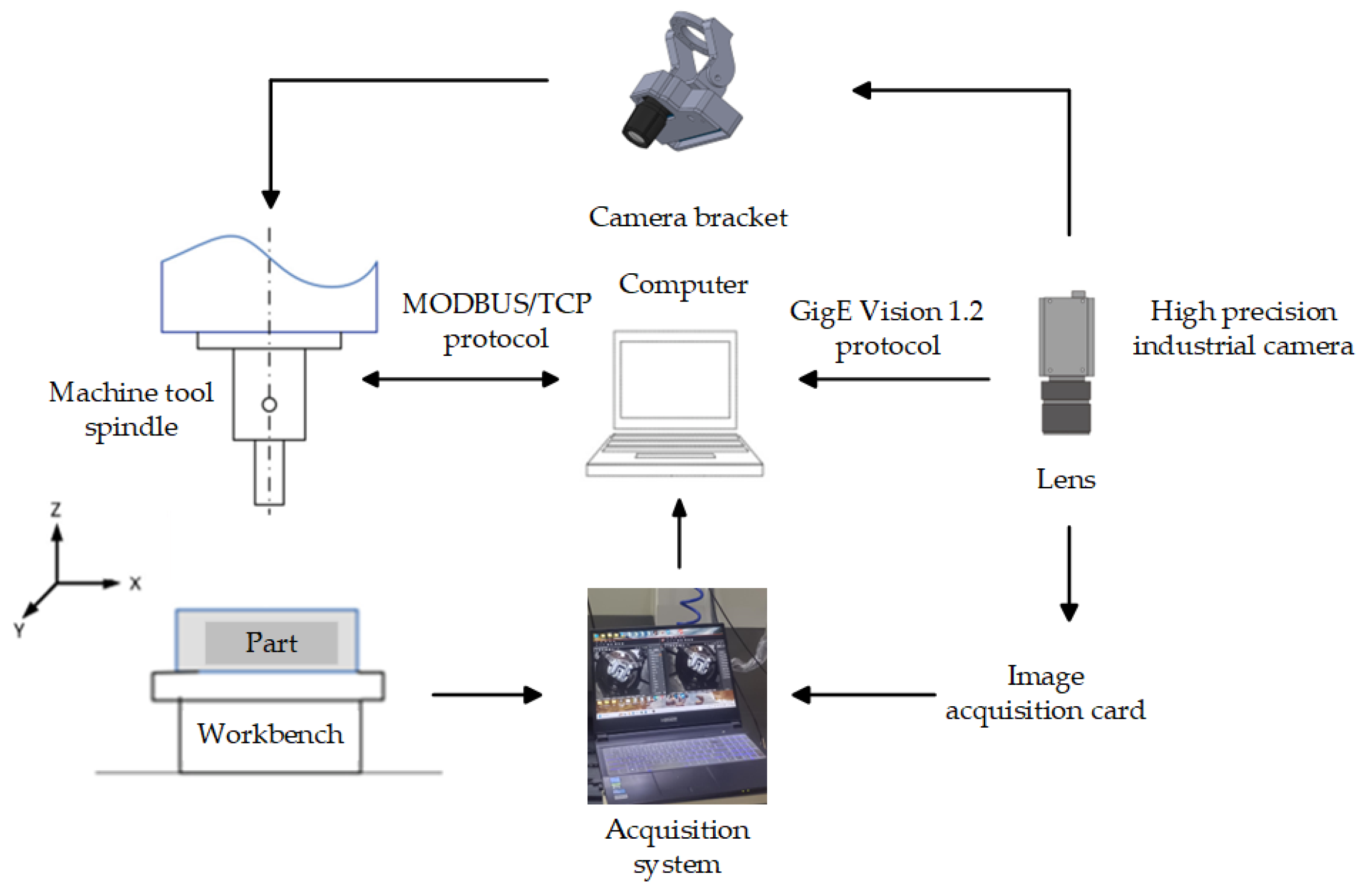
3.1. Experimental Environment Configuration

To verify the effectiveness and real-time capability of the measurement method, a vision measurement experimental platform was designed in this study. This platform utilizes an industrial camera for real-time monitoring and measurement feedback of parts. As shown in Figure 9, the platform consists of a CNC milling machine, a computer (Windows 11, Processor: 11th Gen Intel(R) Core (TM) i5-11260H @ 2.60 GHz 2.61 GHz, Memory: 16 GB (Intel, Santa Clara, CA, USA)), a lens (Model: MVL-MF1618M-5MPE), a Hikvision MV-CA060-11GM (Hangzhou, China) black-and-white industrial camera (specific parameters detailed in

Table 1. Camera Equipment Models and Technical Parameters.

Camera	Model: MV-CA060-11GM
	Light-Sensitive Chips	Photoreceptor Cell	Highest Resolution	High Frame Frequency	Overall Dimensions
	1/1.8 in.	3.75 × 3.75 µm	3072 × 2048 pixel	17 f/s	29 × 29 × 29 mm

), and a light source (Model: MV-LRDS-H-200-90-W2). The specific settings are as follows:

• The industrial camera is connected to the computer via a common GigE interface using a cable, allowing data transmission and control between the camera and the computer.
• The industrial camera is mounted above the machining area of the CNC milling machine, securely fixed using a bracket. This setup allows the camera to capture real-time image data of machined parts, providing data support for subsequent image processing and measurement.
• The parts to be machined are placed on the work table of the CNC milling machine, ensuring that the camera can capture the parts to be measured. This ensures that the position and orientation of the parts remain relatively stable during each machining process.
• On the constructed experimental platform, the method described in this paper is used for real-time image acquisition, edge extraction, and dimension measurement of the parts being machined. By comparing the measurement results with the actual dimensions, the performance and applicability of the algorithm are verified.

To capture the dimensions of parts of varying depths, images of 10 calibration plates need to be captured from different spatial positions. The Zhang calibration method is used to calibrate the camera’s internal parameters. Images of the calibration board are obtained by placing it in 10 different positions in space. MATLAB’s (version: R2024a) Bouguet toolkit is used to detect pixel coordinates of corner points on the target plane in all images. The relationship between the distances from images of different depths to the industrial camera and the scale of a single pixel is calculated to establish the relationship between the actual measured objects and pixel sizes in the image, as shown in Equation (21).

$$\phi =\frac{d_{mean}}{d_n}$$

(21)

where d_mean is the distance between dimension features, d_n is the true length of dimension features, and φ is the calibration coefficient of the system.

To validate the accuracy of the method, the computed results from different algorithms are compared with experimental measurements. Given that the positioning accuracy of the bridge-type coordinate measuring machine is ±2 μm, whereas the camera used in this study achieves a maximum single-pixel precision of ±20 μm, experimental measurements using a Savant bridge-type coordinate measuring machine are employed as the measurement standard to ensure part accuracy, as illustrated in Figure 10. Comparative experiments were conducted on various samples to validate the effectiveness of the method proposed in this study, including coordinate measurements, the algorithm proposed in this study, the Canny edge detection algorithm, the sub-pixel edge detection algorithm [29], and the Otsu–Canny edge detection algorithm [30].

3.2. Measurement of Box Components

3.2.1. Measurement Experiment of Box Components

In image space, the pixel distance between two lines and the distance from the center to the line can be calculated using the Euclidean distance formula. The pixel distance between two lines and the distance from the center of the circle to the line is calculated using the Euclidean distance formula. The Euclidean distance between a line in a given image and a point on another line can be calculated using the following formula:

$$l_E=\frac{\left|A{x}_0+B{y}_0+C\right|}{sqrt\left(A^2+B^2\right)}$$

(22)

where the coordinates of the points on the line are (x₀, y₀), l_E represents the distance from the point to the line, |Ax₀ + By₀ + C| represents the vertical distance from the point to the line, and sqrt (A² + B²) is the modulus of the line. Pixel distance is converted to actual distance based on the actual distance of each pixel.

The relative precision of the parts is calculated as follows:

$$R_a=\frac{\left(l_1-l_2\right)}{l_2}$$

(23)

where R_a represents the relative precision of the algorithm in this article with respect to the coordinate measuring machine, l₁ represents the size obtained by the algorithm in this article, and l₂ represents the size obtained by the coordinate measuring machine.

To verify the reliability of the measurement method, five component specimens were selected for experiments. The length and width of the inner groove of the part, as well as the center distance from the center hole to the outer edge, were measured. The measurement position is shown in Figure 11.

3.2.2. Results Analysis

Using the measurement method designed in this study, images were captured and the length of each specimen was measured. Visual measurement values were obtained based on the method proposed in this study. The values obtained were compared with those from a coordinate measuring machine with micrometer precision, serving as the standard. The comparison includes the results with the Canny edge detection algorithm, the sub-pixel edge detection algorithm, and the Otsu–Canny edge detection algorithm. The experimental results are shown in

Table 2. Statistical Table of Measurement Results.

Measurement Position	Part	Three Coordinate Measuring Machine (mm)	This Article’s Algorithm (mm)	Sub-Pixel Edge Detection Algorithm (mm)	Otsu–Canny Edge Detection Algorithm (mm)	Canny Edge Detection Algorithm (mm)
Length of the inner groove	part 1	43.993	43.979	45.374	43.938	43.997
	part 2	44.005	43.989	44.823	44.324	44.118
	part 3	44.042	44.048	44.616	42.153	44.152
	part 4	44.027	44.044	44.099	42.687	44.100
	part 5	44.005	44.018	43.961	44.031	44.200
Width of the inner groove	part 1	30.002	29.991	29.664	29.096	30.060
	part 2	29.980	29.991	28.596	29.974	29.991
	part 3	30.026	30.022	30.319	30.043	30.181
	part 4	30.017	29.991	29.761	29.233	29.991
	part 5	30.008	29.991	28.010	30.009	30.043
Distance from the circle to the edge	part 1	30.588	30.554	30.564	30.549	37.349
	part 2	30.581	30.711	30.498	30.576	30.047
	part 3	30.496	30.411	30.318	30.623	35.380
	part 4	30.496	30.501	30.569	30.551	28.858
	part 5	30.591	30.581	30.646	30.676	17.724

In the table, the best relative precision is in bold.

.

The experimental results comparing this study with other algorithms are shown in Table 2. From the table, it can be seen that the measurement accuracy of the algorithm in this study is closest to that of the coordinate measuring machine, with a measurement of 30.501 mm and a relative error of 0.005 mm. By comparing the accuracies in Table 2, it can be observed that the highest accuracy of the sub-pixel edge detection algorithm is 43.961 mm, with a relative error of 0.02 mm, which shows a larger measurement error compared to the method proposed in this study. There is a noticeable measurement fluctuation from the center point of the central hole to the outer contour. This is due to the rough machining of the part’s outer surface and low machining accuracy, leading to significant fluctuations in the distance between the hole and the outer contour in the image.

Compared to the sub-pixel edge detection algorithm and the Otsu–Canny edge detection algorithm, the algorithm proposed in this study exhibits satisfactory measurement results. The use of ROI edge detection technology enables the extraction of target information from the ROI edges, thereby avoiding interference from irrelevant areas and improving measurement accuracy. The edge model can better describe the edge characteristics of the part, and when combined with weighted median filtering, it can effectively remove noise, thereby comprehensively improving measurement accuracy. Noise sources such as machining marks produced during the part’s manufacturing process are considered to prevent deviations in visual measurements in actual production processes due to surface marks. This study investigated and analyzed these factors, demonstrating their comprehensive application in real scenarios. The algorithm exhibits excellent performance in terms of measurement accuracy and adaptability, highlighting the superiority of the algorithm design compared to similar applications.

3.3. Measurement of Rectangular Sealing Gaskets

3.3.1. Measurement of Straightness of Rectangular Sealing Gaskets

Directness is defined as the difference between the maximum distance and the minimum distance between the two closest planes. This definition is based on measuring the distances from each point on the workpiece surface to these two planes, used to quantify the linearity of the workpiece surface. Figure 12 utilizes the contour point set of a rectangular sealing piece workpiece (x_i, y_i) to form a set of data points, where i = 1, 2,..., n. These points represent the coordinates on the workpiece surface or contour line. Initially, these data points are fitted into contour lines using the least squares method to ensure that the fitted line closely approximates the actual data points.

$$S(m,c)={{\displaystyle \sum _{i=1}^n(y_i-(m{x}_i+c))}}^2$$

(24)

where m is the slope and c is the intercept. S(m, c) represents the sum of squared errors that need to be minimized with respect to m and c.

By taking partial derivatives of S(m, c) with respect to m and c, and setting them equal to zero, we can obtain the estimated values of the slope m and intercept c for the best-fit line:

$$c=\frac{n{\displaystyle {\sum }_{i=1}^n{x}_i{y}_i-({\displaystyle {\sum }_{i=1}^n{x}_i})({\displaystyle {\sum }_{i=1}^n{y}_i})}}{n{\displaystyle {\sum }_{i=1}^n{x}_i^2-{({\displaystyle {\sum }_{i=1}^n{x}_i})}^2}}$$

(25)

$$c=\frac{{\displaystyle {\sum }_{i=1}^n{y}_i-m{\displaystyle {\sum }_{i=1}^n{x}_i}}}{n}$$

(26)

Once the slope m and intercept c of the best-fit line are obtained, the perpendicular distance d_i from each data point to the line can be calculated. Subsequently, the maximum and minimum distances can be determined:

$$d_i=\frac{\left|m{x}_i-y_i+c\right|}{\sqrt{m^2+1}}$$

(27)

$$\mathrm{Straightness}=\max (d_i)-\min (d_i)$$

(28)

Finally, the calculated straightness value is used to assess the straightness quality of the workpiece surface. A smaller straightness value indicates a smoother and straighter workpiece surface, while a larger straightness value may indicate significant curvature or waviness on the surface.

3.3.2. Analysis of Processing Results

To evaluate the straightness error in this study, comparisons were made with data from the Otsu–Canny edge detection algorithm and the sub-pixel edge detection algorithm, with the results shown in

Table 3. Comparison Table of Straightness Results.

Measurement Position	Part	Three Coordinate Measuring Machine (mm)	This Article’s Algorithm (mm)	Sub-Pixel Edge Detection Algorithm (mm)	Otsu–Canny Edge Detection Algorithm (mm)	Canny Edge Detection Algorithm (mm)
straightness of the outside line 1	part 1	0.015	0.014	0.013	0.018	0.021
	part 2	0.044	0.050	0.057	0.041	0.059
	part 3	0.031	0.037	0.082	0.045	0.042
	part 4	0.029	0.026	0.036	0.040	0.052
	part 5	0.052	0.049	0.060	0.077	0.072
straightness of the outside line 2	part 1	0.047	0.043	0.039	0.041	0.041
	part 2	0.027	0.031	0.021	0.037	0.035
	part 3	0.040	0.043	0.066	0.048	0.051
	part 4	0.059	0.052	0.050	0.049	0.050
	part 5	0.047	0.038	0.046	0.040	0.042
straightness of the straight lines inside 1	part 1	0.035	0.036	0.038	0.037	0.040
	part 2	0.017	0.023	0.029	0.038	0.025
	part 3	0.015	0.025	0.023	0.026	0.030
	part 4	0.026	0.025	0.020	0.031	0.033
	part 5	0.027	0.033	0.033	0.040	0.043
straightness of the straight lines inside 2	part 1	0.030	0.026	0.038	0.030	0.036
	part 2	0.046	0.040	0.063	0.061	0.066
	part 3	0.016	0.026	0.038	0.028	0.035
	part 4	0.018	0.014	0.028	0.032	0.029
	part 5	0.023	0.033	0.033	0.037	0.040

In the table, the best relative precision is in bold.

. The results of the proposed approach are superior to those of the other three methods, with a relative error of 97% compared to the measurements of the coordinate measuring machine. Therefore, the method proposed in this study can be used to assess straightness errors in parts effectively.

3.4. Measurement of Flange Workpieces

3.4.1. Measurement of Roundness of Flange Workpiece

Roundness is a measurement criterion used to describe the deviation of a circular workpiece or component from an ideal circle. It is typically defined as the difference between the maximum and minimum distances from each point on the workpiece surface to its best-fit circle. As shown in Figure 13, the contour point set of a flange workpiece forms a set of data points (x_i, y_i), where i = 1, 2,···, n, representing coordinates on the circular workpiece surface. Assuming a circular model, these data points are fitted using the least squares method. The objective of the least squares method is to find the best-fit circle that minimizes the fitting error in terms of its center and radius. Initially, these data points are fitted into contour lines using the least squares method to ensure that the fitted line closely approximates the actual data points.

$$S(a,b,R)={{\displaystyle \sum _{i=1}^n({(x_i-a)}^2+{(y_i-b)}^2+R^2)}}^2$$

(29)

where (a, b) are the coordinates of the circle’s center, and R is the radius of the circle. S(a, b, R) represents the sum of squared errors that need to be minimized with respect to a, b, and R.

By taking partial derivatives of S(a, b, R) with respect to a, b, and R, and setting them equal to zero, we can obtain the estimated values of the circle’s center coordinates a and b, as well as the radius R for the best-fit circle:

$$a=\frac{{\displaystyle {\sum }_{i=1}^n{x}_i((x_i-\overline{x})(x_i^2+y_i^2-{\overline{x}}^2-{\overline{y}}^2))}}{{\displaystyle {\sum }_{i=1}^n{(x_i^2+y_i^2-{\overline{x}}^2-{\overline{y}}^2)}^2}}$$

(30)

$$b=\frac{{\displaystyle {\sum }_{i=1}^n{y}_i((y_i-\overline{y})(x_i^2+y_i^2-{\overline{x}}^2-{\overline{y}}^2))}}{{\displaystyle {\sum }_{i=1}^n{(x_i^2+y_i^2-{\overline{x}}^2-{\overline{y}}^2)}^2}}$$

(31)

$$R=\sqrt{\frac{1}{n}{\displaystyle \sum _{i=1}^n({(x_i-a)}^2+{(y_i-b)}^2)}}$$

(32)

where x, y are the mean values of the data points.

Once the center coordinates a, b, and radius R of the best-fit circle are obtained, the perpendicular distance di from each data point to the fitted circle can be calculated. Subsequently, the maximum and minimum distances can be determined:

$$d_i=\left|\sqrt{{(x_i-a)}^2+{(y_i-b)}^2}-R\right|$$

(33)

$$\mathrm{roundness}=\max (d_i)-\min (d_i)$$

(34)

Through the above steps, the least squares method can be used to fit a circle and evaluate the roundness of the workpiece surface by calculating distances.

3.4.2. Analysis of Measurement Results

As shown in

Table 4. Comparison Table of Roundness Results.

Measurement Position	Part	Three Coordinate Measuring Machine (mm)	This Article’s Algorithm (mm)	Sub-Pixel Edge Detection Algorithm (mm)	Otsu–Canny Edge Detection Algorithm (mm)	Canny Edge Detection Algorithm (mm)
Inner roundness	part 1	0.067	0.062	0.061	0.050	0.052
	part 2	0.062	0.068	0.063	0.130	0.048
	part 3	0.069	0.062	0.079	0.092	0.095
	part 4	0.043	0.043	0.708	0.069	0.057
	part 5	0.070	0.072	0.068	0.082	0.078
Outer roundness	part 1	0.073	0.780	0.075	0.126	0.095
	part 2	0.082	0.070	0.026	0.022	0.042
	part 3	0.076	0.073	0.097	0.058	0.062
	part 4	0.077	0.070	0.039	0.031	0.035
	part 5	0.070	0.062	0.076	0.067	0.073

In the table, the best relative precision is in bold.

, the algorithm developed in this study exhibits higher accuracy in detecting and measuring roundness features, effectively capturing and analyzing circular contours. By employing weighted median filtering, it successfully reduces the impact of image noise and artifacts on measurement results. The use of ROI edge detection technology ensures that only relevant edge information is extracted, minimizing interference from unrelated areas and thereby enhancing the accuracy of roundness measurements. This demonstrates the effectiveness of the proposed method in roundness measurement.

3.5. ROI Edge Extraction Analysis

As shown in the comparison of edge detection times in Figure 14, when processing a 6144 × 4096 high-resolution image, the fastest measurement times for the sub-pixel edge detection algorithm and the Otsu–Canny edge detection algorithm are 0.17 s and 1.57 s, respectively. In contrast, the fastest test time for our algorithm is 0.16 s, which is faster than the other three detection methods. The first two edge detection methods scan the entire image, requiring the processing of large amounts of data, computation, and time. In comparison, our method accurately locates and extracts the ROI in the image through CAD model drawings. By reducing the processing scope and computational complexity, a faster processing speed is achieved. The targeted ROI processing reduces the impact of pattern processing and uneven illumination on the ROI area. Only the edge features related to part size measurement are processed, eliminating the need to handle background noise and other infrared-related areas, thereby improving edge recognition accuracy. This provides reliable data support for subsequent size measurements and defect detection.

4. Conclusions

This study proposes a method for automatically measuring dimensional features using image processing techniques using machining feature models. First, the ROI of the part is extracted through the machining features of the model. Next, a local image coordinate system is established for measuring the end face to reduce the impact of machining patterns on measurement accuracy. Based on measuring the local coordinates of the part edges, an improved ROI edge detection is used to obtain the diameter of the measuring hole and the distance feature from the center to the center edge. This paper introduces line and circle detection methods based on the Hough transform, which realizes the positioning of part edges and circular holes and establishes dimensional measurement relationships. Finally, the effectiveness of this method was verified by experiments.

(1)

The developed image acquisition system can perform real-time image capture during the manufacturing process of parts. By utilizing methods such as ROI extraction, image deblurring, denoising, and edge detection, the system can complete detection within 0.16 s, achieving clear workpiece contours and excellent detection speed.

(2)

Compared to the measurements of a coordinate measuring machine, the developed measurement method in this study achieved a relative accuracy of 97% for straightness and 96% for roundness.

(3)

Experimental results show that the relative accuracy between the inner groove measured in this study and the measurement results of the coordinate measuring machine reached 99%. In addition, the detection results were analyzed and compared, summarizing the factors that affect the detection accuracy of this method.

References

1. Zhou, G.; Zhang, C.; Li, Z.; Ding, K.; Wang, C. Knowledge-driven digital twin manufacturing cell towards intelligent manufacturing. Int. J. Prod. Res. 2020, 58, 1034–1051. [Google Scholar] [CrossRef]
2. Serrano-Ruiz, J.C.; Mula, J.; Poler, R. Job shop smart manufacturing scheduling by deep reinforcement learning. J. Ind. Inf. Integr. 2024, 38, 100582. [Google Scholar] [CrossRef]
3. Gao, W.; Haitjema, H.; Fang, F.Z.; Leach, R.K.; Cheung, C.F.; Savio, E.; Linares, J.M. On-machine and in-process surface metrology for precision manufacturing. Cirp Ann.-Manuf. Technol. 2019, 68, 843–866. [Google Scholar] [CrossRef]
4. Peng, Y.; Huang, X.; Li, S.G. A measurement point planning method based on lidar automatic measurement technology. Rev. Sci. Instrum. 2023, 94, 015104. [Google Scholar] [CrossRef] [PubMed]
5. Li, Y. Application of Computer Vision in Intelligent Manufacturing under the Background of 5G Wireless Communication and Industry 4.0. Math. Probl. Eng. 2022, 2022, 9422584. [Google Scholar] [CrossRef]
6. Yang, J.C.; Wang, C.G.; Jiang, B.; Song, H.B.; Meng, Q.G. Visual Perception Enabled Industry Intelligence: State of the Art, Challenges and Prospects. IEEE Trans. Ind. Inform. 2021, 17, 2204–2219. [Google Scholar] [CrossRef]
7. Pan, L.; Sun, G.D.; Chang, B.F.; Xia, W.; Jiang, Q.; Tang, J.W.; Liang, R.H. Visual interactive image clustering: A target-independent approach for configuration optimization in machine vision measurement. Front. Inf. Technol. Electron. Eng. 2023, 24, 355–372. [Google Scholar] [CrossRef]
8. Wang, S.; Kobayashi, Y.; Ravankar, A.A.; Ravankar, A.; Emaru, T. A Novel Approach for Lidar-Based Robot Localization in a Scale-Drifted Map Constructed Using Monocular SLAM. Sensors 2019, 19, 2230. [Google Scholar] [CrossRef]
9. Cui, G.T.; Wang, J.Z.; Li, J. Robust multilane detection and tracking in urban scenarios based on LIDAR and mono-vision. IET Image Process. 2014, 8, 269–279. [Google Scholar] [CrossRef]
10. Huang, L.Q.; Zhe, T.; Wu, J.Y.; Wu, Q.; Pei, C.H.; Chen, D. Robust Inter-Vehicle Distance Estimation Method Based on Monocular Vision. IEEE Access 2019, 7, 46059–46070. [Google Scholar] [CrossRef]
11. Ma, Y.B.; Zhao, R.J.; Liu, E.H.; Zhang, Z.; Yan, K. A novel autonomous aerial refueling drogue detection and pose estimation method based on monocular vision. Measurement 2019, 136, 132–142. [Google Scholar] [CrossRef]
12. Sun, S.Y.; Yin, Y.J.; Wang, X.G.; Xu, D. Robust Landmark Detection and Position Measurement Based on Monocular Vision for Autonomous Aerial Refueling of UAVs. IEEE Trans. Cybern. 2019, 49, 4167–4179. [Google Scholar] [CrossRef]
13. Sun, Y.; Wang, X.X.; Lin, Q.X.; Shan, J.H.; Jia, S.L.; Ye, W.W. A high-accuracy positioning method for mobile robotic grasping with monocular vision and long-distance deviation. Measurement 2023, 215, 112829. [Google Scholar] [CrossRef]
14. Bai, R.; Jiang, N.; Yu, L.; Zhao, J. Research on industrial online detection based on machine vision measurement system. J. Phys. Conf. Ser. 2021, 2023, 012052. [Google Scholar] [CrossRef]
15. Zhang, Z.Y.; Wang, X.D.; Zhao, H.T.; Ren, T.Q.; Xu, Z.; Luo, Y. The Machine Vision Measurement Module of the Modularized Flexible Precision Assembly Station for Assembly of Micro- and Meso-Sized Parts. Micromachines 2020, 11, 918. [Google Scholar] [CrossRef] [PubMed]
16. Feldhausen, T.; Heinrich, L.; Saleeby, K.; Burl, A.; Post, B.; MacDonald, E.; Saldana, C.; Love, L. Review of Computer-Aided Manufacturing (CAM) strategies for hybrid directed energy deposition. Addit. Manuf. 2022, 56, 102900. [Google Scholar] [CrossRef]
17. Angrisani, L.; Daponte, P.; Liguori, C.; Pietrosanto, A. An automatic measurement system for the characterization of automotive gaskets. In Proceedings of the IEEE Instrumentation and Measurement Technology Conference Sensing, Processing, Networking, IMTC Proceedings, Ottawa, ON, Canada, 19–21 May 1997; pp. 434–439. [Google Scholar] [CrossRef]
18. Nogueira, V.V.E.; Barca, L.F.; Pimenta, T.C. A Cost-Effective Method for Automatically Measuring Mechanical Parts Using Monocular Machine Vision. Sensors 2023, 23, 5994. [Google Scholar] [CrossRef] [PubMed]
19. Liu, S.Y.; Ge, Y.P.; Wang, S.; He, J.L.; Kou, Y.; Bao, H.J.; Tan, Q.C.; Li, N. Vision measuring technology for the position degree of a hole group. Appl. Opt. 2023, 62, 869–879. [Google Scholar] [CrossRef]
20. Fu, X.G.; Li, H.; Zuo, Z.J.; Pan, L.B. Study of real-time parameter measurement of ring rolling pieces based on machine vision. PLoS ONE 2024, 19, e0298607. [Google Scholar] [CrossRef]
21. Salah, M.; Ayyad, A.; Ramadan, M.; Abdulrahman, Y.; Swart, D.; Abusafieh, A.; Seneviratne, L.; Zweiri, Y. High speed neuromorphic vision-based inspection of countersinks in automated manufacturing processes. J. Intell. Manuf. 2023. [Google Scholar] [CrossRef]
22. Huang, M.L.; Liu, Y.L.; Yang, Y.M. Edge detection of ore and rock on the surface of explosion pile based on improved Canny operator. Alex. Eng. J. 2022, 61, 10769–10777. [Google Scholar] [CrossRef]
23. Ranjan, R.; Avasthi, V. Edge Detection Using Guided Sobel Image Filtering. Wirel. Pers. Commun. 2023, 132, 651–677. [Google Scholar] [CrossRef]
24. Xiao, G.F.; Li, Y.T.; Xia, Q.X.; Cheng, X.Q.; Chen, W.P.; Cheng, X.Q.; Chen, W.P. Research on the on-line dimensional accuracy measurement method of conical spun workpieces based on machine vision technology. Measurement 2019, 148, 106881. [Google Scholar] [CrossRef]
25. Jiang, B.C.; Du, X.; Wu, L.L.; Zhu, J.W. Visual measurement of the bearing diameter based on the homography matrix and partial area effect. Proc. Inst. Mech. Eng. Part C-J. Mech. Eng. Sci. 2024, 238, 2034–2043. [Google Scholar] [CrossRef]
26. Li, B. Research on geometric dimension measurement system of shaft parts based on machine vision. Eurasip J. Image Video Process. 2018, 2018, 101. [Google Scholar] [CrossRef]
27. Gao, C.; Zhou, R.G.; Li, X. Quantum color image scaling based on bilinear interpolation. Chin. Phys. B 2023, 32, 050303. [Google Scholar] [CrossRef]
28. Zhang, Q.; Xu, L.; Jia, J. 100+ times faster weighted median filter (WMF). In Proceedings of the IEEE Conference on Computer Vision and Pattern Recognition, Columbus, OH, USA, 23–28 June 2014; pp. 2830–2837. [Google Scholar] [CrossRef]
29. Gioi, R.G.V.; Randall, G. A Sub-Pixel Edge Detector: An Implementation of the Canny/Devernay Algorithm. Image Process. Line 2017, 7, 347–372. [Google Scholar] [CrossRef]
30. Cao, J.F.; Chen, L.C.; Wang, M.; Tian, Y. Implementing a Parallel Image Edge Detection Algorithm Based on the Otsu-Canny Operator on the Hadoop Platform. Comput. Intell. Neurosci. 2018, 2018, 3598284. [Google Scholar] [CrossRef]
Figure 1. Algorithm flowchart.
Applsci 14 06094 g001
Figure 2. Bilinear interpolation calculation: (a) original pixel image; (b) bilinear interpolation of the pixel image.
Applsci 14 06094 g002
Figure 3. Feature model: The arc features are the center point A, the starting point B, and the curvature 180°. The straight-line features are the starting point B and the ending point C.
Applsci 14 06094 g003
Figure 4. Filling of image: Image (a) results in Image (b) after filling.
Applsci 14 06094 g004
Figure 5. Feature-Model-based ROI: Red areas are the ROI, and black areas represent the machining feature models.
Applsci 14 06094 g005
Figure 6. Linear parameter representation and parameter space: (a) image space; (b) parameter space.
Applsci 14 06094 g006
Figure 7. Linear parameter representation and polar coordinate parameter space: (a) image space; (b) parameter space.
Applsci 14 06094 g007
Figure 8. Transform Circle Detection Representation: (a) image space; (b) parameter space.
Applsci 14 06094 g008
Figure 9. On-machine detection equipment.
Applsci 14 06094 g009
Figure 10. Three-coordinate measuring instrument: (a) coordinate measuring machine; (b) measurement software; (c) measuring head.
Applsci 14 06094 g010
Figure 11. The detection position of the part.
Applsci 14 06094 g011
Figure 12. Diagram of rectangular sealing gasket sample detection.
Applsci 14 06094 g012
Figure 13. Diagram of flange workpiece sample detection.
Applsci 14 06094 g013
Figure 14. Edge detection time comparison chart.
Applsci 14 06094 g014