Virtual Streamline Traction: Formation Cooperative Obstacle Avoidance Based on Dynamical Systems

Abstract

Formation obstacle avoidance is a critical aspect of cooperation among unmanned surface vehicles (USVs). In practical scenarios involving multiple USVs, managing obstacle avoidance during formation assembly and navigation is essential to ensure the success of cooperative tasks. This study devised a formation cooperative obstacle-avoidance scheme utilizing dynamical systems (DS). The traditional interfered fluid dynamical system (IFDS) applied in two-dimensional planes was enhanced to address local minima issues. Furthermore, robust virtual structure patterns were implemented to effectively decouple velocity vectors. Streamlines were optimized by adjusting velocity amplitudes within specific distance intervals, facilitating precise formation assembly amidst multiple obstacles. Additionally, a novel inter-vehicle disturbance method, distinct from the IFDS, was developed to enhance inter-vehicle collision avoidance. The effectiveness of the proposed method in enabling USV formations to adeptly navigate obstacles while maintaining formation integrity and collision-avoidance capabilities was analyzed theoretically and confirmed through simulation.

1. Introduction

In recent years, the concept of unmanned systems has gained significant traction. Notably, unmanned surface vehicles (USVs) have experienced rapid advancement. As crucial elements of unmanned maritime systems, USVs offer advantages such as high-speed intelligence, compact size, maneuverability, and cost-effectiveness compared to traditional surface vessels [1]. With the diversification of marine operations, the limitations of single-vehicle operations necessitate research into the cooperative use of multiple USVs to enhance operational efficiency and expand operational scopes [2]. The cooperation among multiple USVs finds applications in marine replenishment, waterway security, unmanned combat systems, hydrological and meteorological information gathering, and surface search and rescue. Such cooperation represents a collaborative approach enabling USVs to accomplish complex tasks. As a member of intelligent robots, the importance of obstacle avoidance cannot be overemphasized [3].

Formation cooperative obstacle avoidance is a foundational technology for achieving effective cooperation among multiple USVs [4,5,6].

The following are two practical scenarios in formation obstacle avoidance:

• During the initial stage of task execution by the formation, the primary step involves assembling individual vehicles into a formation—positioning each vehicle at its designated location to establish the shape of the formation. During this process, obstacles along the route of each vehicle and route conflicts between vehicles may lead to collisions. To enhance the efficiency of task execution by the formation, a dynamic process is preferred, where formation assembly and task execution occur synchronously rather than waiting for all vehicles to come into formation before commencing task execution.
• During the task execution by the formation, obstacles may be encountered along the route. Therefore, the formation should rationally avoid obstacles while ensuring a safe distance between vehicles. Following avoidance, the formation may be recovered. Given the surface motion characteristics of USVs, obstacle avoidance should be conducted without sacrificing formation robustness and efficiency. Thus, a robust and efficient virtual guidance structure is preferred [7,8]. However, virtual structure patterns have apparent drawbacks: their poor adaptability is unfavorable for obstacle avoidance. The obstacle avoidance in the virtual structure formation method typically involves the entire formation avoiding obstacles, with members of high mobility cooperating with those of low mobility to maintain the formation. However, this cooperation reduces the flexibility of each member within the formation. Consequently, it may result in an increased total path for obstacle avoidance, particularly when dealing with small groups of obstacles. Members with high mobility can traverse such obstacle groups without detouring. To minimize unnecessary trips and enhance task efficiency, we seek a novel solution to address the limited flexibility inherent in the virtual deconstruction method.

To address these drawbacks, a series of targeted explorations were conducted. Mainstream obstacle-avoidance solutions include the following:

• The most traditional approach is one based on geometry; among many categories, the more classic is the velocity obstacle (VO) method [9,10,11,12].
• Model predictive control (MPC) [13,14,15], where [13] utilizes MPC for quadratic programming on intended velocities for obstacle avoidance, and [14] employs MPC to address collision-avoidance issues within formations.
• Based on probability or Stochastic planning methods, rapidly exploring random trees (RRT) algorithm and its variants are common [16,17].
• Artificial potential field (APF) methods [18,19,20], with [19,20] using consensus algorithms alongside APF to achieve intra-formation collision avoidance and formation obstacle avoidance.
• Methods based on machine learning, including deep learning and reinforcement learning [21,22,23].

While geometry-based methods offer simplicity and good integrative capabilities, they often fail to yield satisfactory results when faced with complex obstacles, particularly as they struggle to adapt quickly to environmental changes in dynamic settings. The primary drawback of MPC and stochastic planning methods is the exponential increase in computational complexity with the addition of control dimensions, rendering these methods computationally inefficient during obstacle avoidance. Machine learning-based methods provide significant advantages in handling nonlinear, non-stationary, and complex tasks but suffer from poor portability and low sample efficiency. Furthermore, these methods are sensitive to noise and lack practical applicability. APF is highly practical but suffers from numerous local minima issues and poor stability, as depicted in

Table 1. Current mainstream solutions to the obstacle-avoidance problem.

Solution	Instance	Disadvantage
Based on geometric analysis methods	Velocity obstacle method	Unable to adapt quickly to changes in dynamic environments
Model predictive control (MPC) methods	Nonlinear MPC method	High computational requirements and workload; low computational efficiency
Stochastic planning methods	Rapidly exploring random-tree algorithm	Low calculation efficiency in complex environments
Methods of simulating force fields	Artificial potential field (APF) method	Many local minima problems
Intelligent optimization algorithms	Neural networks and reinforcement learning	Sample inefficiency and generalizability problems; poor practicality

.

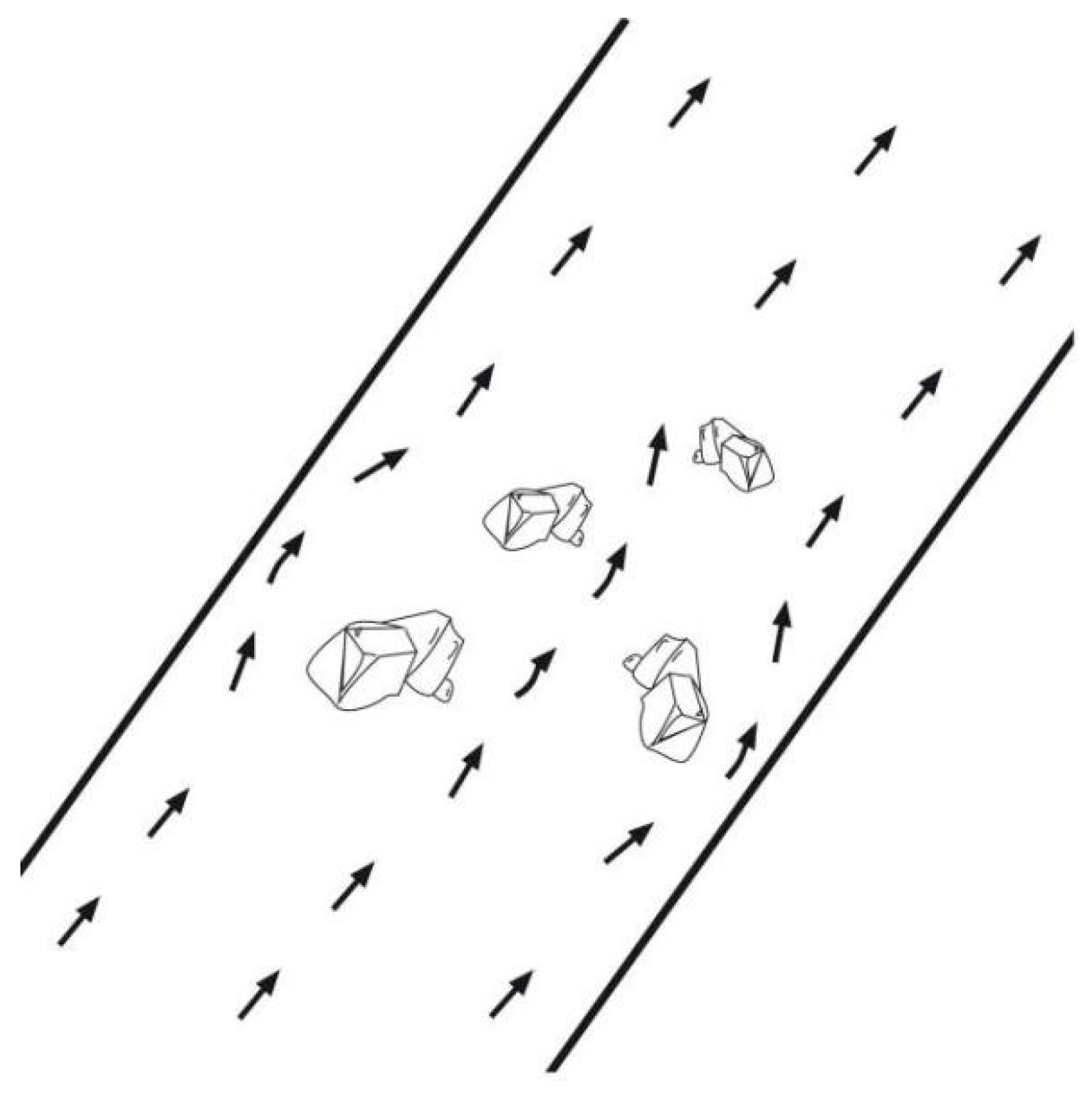
Inspired by the natural avoidance of obstacles by flowing water, as depicted in Figure 1, the continuous flow of water prompts scholars to select the velocity vector of a particle in the flow field at different observation times as a correspondence to the agent’s velocity vector, thereby achieving the nonlinear simulation of water flow and avoidance of obstacles. Various methods can simulate obstacle-avoidance behavior of water flow, including those based on stream functions. Notably, the interfered fluid dynamical system (IFDS) [24,25,26,27,28], grounded in dynamical systems (DSs) [29], offers significant advantages. The IFDS algorithm exhibits low computational complexity and yields smooth trajectory solutions [28]. This approach is particularly suitable for certain underactuated USVs that lack lateral thrust. Its practicality is further enhanced by the optimized velocity vectors it produces. Unlike the vector-field approach of APF, the IFDS encounters fewer problems with local minima and demonstrates superior obstacle-avoidance capabilities, as elaborated in [26] and subsequent studies. Despite these strengths, the IFDS still faces challenges in two-dimensional obstacle avoidance and in its application to USV formations. Addressing these limitations, this study developed a combined IFDS and DS methodology, termed the virtual streamline traction (VST) method. This novel approach enhances IFDS by overcoming its two-dimensional constraints, incorporating an innovative formation strategy based on an improved IFDS, and devising a novel collision-avoidance technique for formation members using DS. This culminates in a robust and practical formation strategy for USVs.

2. Obstacle-Avoidance Formulation

Consider a USV operating in calm water without obstacles. Let the position of the USV at time t be ${\xi }_t=(x_t,y_t)$ and the target point of its current voyage be ${\xi }_d=(x_d,y_d)$. At this moment, the velocity amplitude of the USV is V. The route is then a straight line between the two points with coordinates ξ_t and ξ_d. The initial flow field $u_t$ in the geodetic coordinate system is as follows:

$$u_t={\left[\begin{array}{cc}\frac{V(x_d-x_t)}{d}& \frac{V(y_d-y_t)}{d}\end{array}\right]}^T,$$

(1)

where $d=\sqrt{{(x_t-x_d)}^2+{(y_t-y_d)}^2}$ is the distance between the position if the USV is at time t and the target point.

When obstacles are encountered, they induce disturbances in the initial flow field, causing the navigation route to deviate from obstacles and eventually converge toward the target. In practical scenarios, employing sensors that detect obstacles with high precision can be challenging. To enhance planning efficiency, obstacles can be represented by their boundary volumes. This approach involves categorizing obstacles into standard convex shapes. For example, geographical features such as islands, reefs, and shorelines may be represented as triangles, rectangles, hexagons, ellipses, and circles, or combinations thereof. Similarly, moving boats and vessels can be simplified into circles and ellipses for ease of modeling. To facilitate a standardized approach to obstacle modeling, the representation of obstacles is uniformly defined as follows [30]:

$$\Gamma (\xi )={(\frac{{\mathrm{x}}_{\mathrm{t}}-{\mathrm{x}}_0}{\mathrm{c}})}^{2a}+{(\frac{y_t-y_0}{d})}^{2b},$$

(2)

where ${\xi }_0=(x_0,y_0)$ is the center of the obstacle, c and d are the axial lengths of the obstacle, and a and b are the shape parameters of the obstacle. This method can construct boundary volumes for most obstacles. Extremely large obstacles can be represented as combinations of multiple obstacles to significantly increase the feasibility of obstacle avoidance routes.

Let $\overline{M}$ represent the disturbances caused by all obstacles to the initial flow field (the velocity vector associated with each point in the original flow field is modulated) [29]. The expression is as follows:

$$\overline{M}={\displaystyle \sum _{k=1}^N{W}_k{M}_k},$$

(3)

where “N” is the total number of obstacles, the letter “k” represents the k-th obstacle, W_k is the weight of the k-th obstacle, and M_k is the disturbance to the initial flow field u_t caused by the k-th obstacle. The expressions for W_k and M_k are as follows:

$$W_k=\left\{\begin{array}{c}1\\ {\displaystyle {\prod }_{i=1,i\ne k}^N\frac{({\Gamma }_i-1)}{({\Gamma }_i-1)+({\Gamma }_k-1)}}\end{array}\begin{array}{c}N=1\\ N\ne 1\end{array}\right.,$$

(4)

$$M_k=I-\frac{n_k{n}_k^T}{{\left|{\Gamma }_k\right|}^{1/{\rho }_k}{n}_k^T{n}_k},$$

(5)

where I is the second-order identity matrix, $-\frac{n_k{n}_k^T}{{\left|{\Gamma }_k\right|}^{1/{\rho }_k}{n}_k^T{n}_k}$ is the disturbance matrix (representing the disturbance to the initial flow field caused by the obstacle), ρ_k is the disturbance coefficient (adjusting the degree of disturbance caused by the obstacles to the initial flow field; the greater the disturbance coefficient ρ_k, the more severe the disturbance caused by the obstacles), and n^k is a vector normal to the surface of the k-th obstacle, $n^k={\left[\begin{array}{cc}\frac{\partial {\Gamma }_k}{\partial x}& \frac{\partial {\Gamma }_k}{\partial y}\end{array}\right]}^{\mathrm{T}}$.

Next, consider the presence of dynamic obstacles such as moving vessels and other mobile platforms. To avoid them, the original flow velocity u_t must be modified as follows:

$$\overline{u_t}=\overline{M}(u_t-v_{\Gamma })+v_{\Gamma }$$

(6)

Here, v_Γ is defined as the total velocity vector of the obstacles.

$$v_{\Gamma }={\displaystyle \sum _{k=1}^N{W}_k{e}^{\frac{1-{\Gamma }_k}{{\lambda }_k}}{v}_{{\Gamma }_k}},$$

(7)

where λ_k is a constant for the k-th obstacle, and $v_{{\Gamma }_k}$ is the velocity vector of the k-th obstacle. Finally, the total flow field ${\overline{u}}_{\mathrm{t}}={\left[\begin{array}{cc}\overline{u_{x_t}}& \overline{u_{y_t}}\end{array}\right]}^{\mathrm{T}}$ is obtained from Equation (6), and the position of the USV at the next moment is updated to ${\xi }_{\mathrm{t}+1}=(x_{t+1},y_{t+1})=(x_t+\overline{u_{x_{\mathrm{t}}}}\Delta t,y_t+\overline{u_{y_t}}\Delta t)$. Integration of the sampling time $\Delta t$ yields route planning for the USV; the shorter the sampling duration, the more precise the planned trajectory.

To verify the feasibility of this method, two assertions must hold true:

• The route leads to the target point.

Proof. 

When the USV is far from all obstacles, the value of ${\Gamma }_k$ will gradually increase, and we can approximately consider ${\Gamma }_k$ to approach infinity when the distance from the obstacle is sufficiently large (${\Gamma }_k\approx \infty$). This implies that the disturbance matrix $-\frac{n_k{n}_k^T}{{\left|{\Gamma }_k\right|}^{1/{\rho }_k}{n}_k^T{n}_k}$ in Equation (5) approaches 0. Therefore, the obstacles do not disturb the initial flow field. The total flow field value stands at ${\overline{u}}_t=u_t$, satisfying the requirement that the route must end at the target point. □

2.

The obstacles are impenetrable.

Proof. 

To ensure the impenetrability of obstacles (the USV does not traverse the obstacle model), it is sufficient to demonstrate that the normal velocity disappears at the surface of the obstacle, i.e., $n_k^T\overline{u_t}=0$ [31]. On the surface of the obstacle, ${\Gamma }_k=1$ and $n_k^T\overline{u_t}=n_k^T{M}_k{u}_t$. Because $n_k^T{M}_k=n_k^T-\frac{n_k^T{n}_k{n}_k^T}{n_k^T{n}_k}=n_k^T-n_k^T=0$, it follows that $n_k^T\overline{u_t}=0$, the velocity vector of the USV at the surface of the obstacle, when projected onto the normal vector direction, becomes zero, meeting the requirement that the obstacles must be impenetrable. □

Therefore, the obstacle-avoidance method ensures that the vehicles eventually reach the target point, even though the obstacles are impenetrable.

3. Local Minima and Solution

To some extent, the aforementioned approach mitigates the various local minima problems that are intrinsic to APF, resulting in smooth obstacle-avoidance routes reminiscent of the way in which water flows around rocks. However, when the above approach is utilized in two-dimensional planes, two types of local minima problems persist: stationary points and trap areas. This section intends to discuss and solve these problems.

3.1. Stationary Points

As shown in Figure 2, when the target point of the USV lies directly behind an obstacle, the USV navigates straight toward the center of the obstacle. In this case, there is collinearity among the USV, obstacle center, and target point. Upon reaching the edge of the obstacle, the USV cannot cross the obstacle in a two-dimensional plane. Therefore, the velocity vector becomes zero on the edge of the obstacle, causing the USV to stall at the edge, creating a stationary point.

It is evident that even minor deviations in heading can enable the USV to evade stationary obstacles effectively. In practice, as illustrated in Figure 2, it is uncommon for a route to maintain a consistent heading; slight alterations in the heading of the USV often occur because of natural influences such as waves and wind during navigation. To mitigate unnecessary risks and building on the aforementioned observations, the disturbance formula was modified by incorporating an offset vector to the surface normal vector of the obstacle. A tangent vector ${\tau }_k={\left[\begin{array}{cc}\frac{\partial {\Gamma }_k}{\partial y}& -\frac{\partial {\Gamma }_k}{\partial x}\end{array}\right]}^{{\rm T}}$ perpendicular to the obstacle’s surface normal vector $n^k$ was selected and incorporated into Equation (5), yielding

$$M_k=I-\frac{n_k{n}_k^T}{{\left|{\Gamma }_k\right|}^{1/{\rho }_k}{n}_k^T{n}_k}+\frac{i{\tau }_k{n}_k^T}{{\left|{\Gamma }_k\right|}^{1/{\sigma }_k}{n}_k^T{n}_k{C}_k},$$

(8)

where the newly added matrix $\frac{i{\tau }_k{n}_k^T}{{\left|{\Gamma }_k\right|}^{1/{\sigma }_k}{n}_k^T{n}_k{C}_k}$ is the disturbance-deviation matrix of the obstacle. By introducing this matrix, the sum of the tangent vector ${\tau }_k$ and the normal vector $n^k$ acts as a disturbance to the initial flow field. Here, $i\in [-1,1]$ can adjust the deviation direction. Proper selection of the value of $i$ enables the USV to deviate right when approaching the right boundary and left when approaching the left boundary. In Equation (8), ${\sigma }_k$ is the deviation coefficient of the k-th obstacle. A larger deviation coefficient leads to earlier avoidance of stationary points. To ensure that the deviation matrix does not affect the obstacle-avoidance effect of the disturbance matrix, a constant $C_k$ is introduced. When this parameter is reasonably set, the norm of the deviation matrix $\frac{i{\tau }_k{\mathrm{n}}_k^T}{{\left|{\Gamma }_k\right|}^{1/{\sigma }_k}{n}_k^T{n}_k{C}_k}$ should be far smaller than that of the disturbance matrix $\frac{n_k{n}_k^T}{{\left|{\Gamma }_k\right|}^{1/{\rho }_k}{n}_k^T{n}_k}$.

3.2. Trap Areas

During the creation of obstacle models, overlapping is commonly observed. At the intersection of two obstacles, both ${\Gamma }_k$ and ${\Gamma }_{k+1}$ become 1. Thus, the denominator of the weight Equation (4) becomes 0, which leads to the failure of navigation planning. As depicted in Figure 3, when a USV continues toward the overlapping region of two obstacles, it can easily become ensnared in the “trap area” formed by these obstacles.

Trap areas are particularly prevalent when constructing models of large-scale obstacles, such as coastal areas and ports. Since these large-scale obstacles often contain multiple smaller obstacles, it is crucial to appropriately fill these trap areas based on the boundary volume of the obstacles to ensure unimpeded navigation. The method for filling these areas is detailed in Figure 4.

The trap-area-filling method effectively addresses all identified trap areas. However, in the expansive maritime environment, obstacles are generally scarce and not overly large, comprising primarily small islands and vessels. Employing the trap-area method might inadvertently enlarge the obstacle volume, leading to deviations from the optimal route. This is particularly problematic for USVs operating at sea, where conditions for replenishing power sources are limited. In such scenarios, adhering to the shortest possible route is paramount. To address these issues, employing a virtual target point is recommended because it offers a solution to the trap-area problems. This approach is illustrated in Figure 5.

When obstacles overlap and the heading of the USV points toward the trap area, it becomes crucial to determine the generation of virtual target points. Initially, upon entering the trap warning area, a sector navigation domain is established based on the angular velocity boundary limit, given the current velocity amplitude. A set of virtual target points, Vir_{1,2,3,4 … P}, on the arc of the sector navigation domain, is obtained (illustrated by the red arc in Figure 5). The selection of reasonable virtual target points is guided by specific criteria, which are detailed as follows:

First, drawing inspiration from articles concerning the presence of radar targets within a specified area [32,33,34], lines l₁ and l₂ are constructed perpendicular to the tangent line at the tangent point. Starting from the virtual target point, a ray is projected onto one of these lines, l₁ and l₂. When the ray intersects both l₁ and l₂, the virtual target point is considered feasible. Conversely, if the ray only intersects with one of the lines l₁ and l₂, the virtual target point is considered unfeasible and is therefore excluded from generating the corresponding feasible domain.

Second, the optimal virtual target point is determined based on the cost function Eva:

$$Eva={\lambda }_1\gamma +{\lambda }_2\chi +{\lambda }_3\mu ,$$

(9)

$$\gamma =\left\{\begin{array}{c}{\displaystyle \prod _{k=1}^{K}1/{\Gamma }_k(Vi{r}_p)}\\ +\infty \end{array}\right.\begin{array}{c}\\ \end{array}\begin{array}{c}\\ \end{array}\begin{array}{c}{\Gamma }_k(Vi{r}_p)>1\\ {\Gamma }_k(Vi{r}_p)\le 1\end{array},$$

$$\chi =\frac{d\left(Vi{r}_p,{\xi }_d\right)-\min d\left(Vi{r}_p,{\xi }_d\right)}{d_{\max }\left(Vi{r}_p,{\xi }_d\right)-\min d\left(Vi{r}_p,{\xi }_d\right)},$$

$$\mu =\left\{\begin{array}{c}0\\ +\infty \end{array}\right.\begin{array}{c}\\ \end{array}\begin{array}{c}\mathrm{Do}\mathrm{not}\mathrm{sail}\mathrm{to}\mathrm{new}\mathrm{trap}\mathrm{areas}\\ Otherwise\end{array},$$

where λ₁, λ₂, and λ₃ are weights. Here, γ is the collision cost (reflecting whether there is a collision with obstacles, where $Vi{r}_p$ corresponds to the coordinates of the virtual target point), χ is the consumption cost (reflecting the magnitude of the additional navigation distance caused by the virtual target point), and μ is the escape cost (reflecting whether the USV is heading toward other trap areas). When the virtual target point satisfies the requirements of the cost function and feasibility, the USV navigates to the selected virtual target point and then heads to the real target point.

The aforementioned ruling renders it impossible to identify any virtual target point that satisfies the given criteria. The velocity amplitude is reduced, and a new sector navigation domain is generated.

4. Disturbance-Based USB Formation Scheme

4.1. Formation Assembly

Based on the previously discussed individual USV obstacle avoidance, the virtual guidance structure was integrated to achieve formation assembly, as shown in Figure 6.

Figure 6 illustrates the assembly strategy. The virtual-structure point (VSP) corresponding to each USV in the formation is taken as the target point in the disturbed flow field. During assembly, the USVs in the formation perceive each other as obstacles according to the hierarchy $US{V}_1>US{V}_2>US{V}_3\dots \dots >US{V}_j$. In other words, $US{V}_2$ perceives $US{V}_1$ as an obstacle, $US{V}_3$ perceives both $US{V}_2$ and $US{V}_1$ as obstacles, and so on. Given the characteristics of the disturbed flow field mentioned in Section 2, this assembly strategy enables SUVs to effectively avoid obstacles and navigate toward their respective formation positions via shorter routes, fulfilling both assembly requirements and addressing concerns of obstacle avoidance and inter-vehicle collision during assembly.

The virtual structure in a specified direction according to the formation task ensures all USVs are linked through the flow lines of the disturbed flow field. This dynamic formation assembly process, analogous to following guiding threads, facilitates formation navigation while overcoming the rigidity of the virtual structure and significantly enhancing the efficiency of task execution.

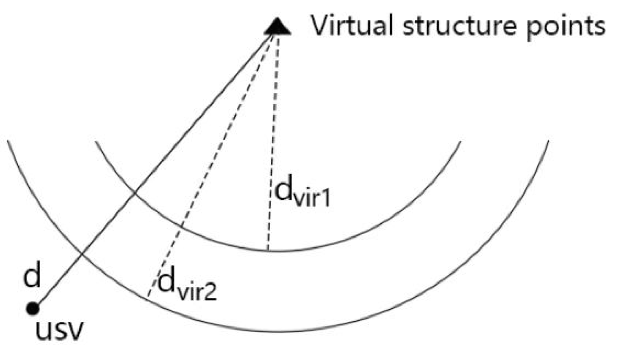
To maintain formation shape, the vector and scalar components of the initial flow field of the individual USV are decoupled. Equation (1) is separated into a velocity vector ${\left[\begin{array}{cc}\frac{x_d-x_t}{d}& \frac{y_d-y_t}{d}\end{array}\right]}^T$ and velocity amplitude $V$ based on the distance to the VSP, as shown in Figure 7.

The relationship between each vehicle’s velocity amplitude and distance to the VSP is expressed as follows:

$$V=\left\{\begin{array}{cc}\begin{array}{c}{V}_{\max }\\ V_{vir}+(V_{\max }-V_{vir})e^{-{\lambda }_{vir2}(d_{vir2}-d)}\\ V_{vir}{e}^{-{\lambda }_{vir1}(d_{vir1}-d)}\end{array}& \begin{array}{c}d>d_{vir2}\\ d_{vir1}<d\le d_{vir2}\\ d\le d_{vir1}\end{array}\end{array}\right.,$$

(10)

where $V_{\max }$ is the maximum velocity amplitude of the vehicle, $V_{vir}$ is the preset velocity toward the VSPs (adjusted based on formation-task requirements), $d_{vir1}$ and $d_{vir2}$ are distance thresholds, $d$ is the distance of the USV to the VSP, and ${\lambda }_{vir1}$ and ${\lambda }_{vir2}$ are constants for adjusting the velocity amplitude. In Formula (10), we can make the preset values of $d_{vir1}$ and $d_{vir2}$ close to each other so that the velocity amplitude can converge faster on the preset speed $V_{vir}$ and keep the distance $d$ between the boat and the virtual structure point within the interval of $d_{vir1}$ and $d_{vir2}$. In Formula (10), when $d=d_{vir2}$, $V=V_{\max }$. When $d\to d_{vir1}$, $V$ converges to $V_{vir}$. When $d=d_{vir1}$, $V=V_{vir}$, Formula (10) can be regarded as a monotonically decreasing continuous function. In order to reduce the vibration of the velocity amplitude when it is constrained and affect the sailing effect, once each USV enters the range between $d_{vir1}$ and $d_{vir2}$ for the first time, it no longer perceives other USVs as obstacles. This ensures that each USV does not affect the others during formation navigation. After all the USVs enter the range between $d_{vir1}$ and $d_{vir2}$, formation assembly transitions to formation navigation.

In summary, a virtual formation is established by connecting USVs and corresponding VSPs through flow lines generated by disturbing the flow field. Through the convergence of the velocity amplitude, the flow lines are tightened similarly to elastic strings so that the USVs maintain their shape and follow the motion of the virtual formation.

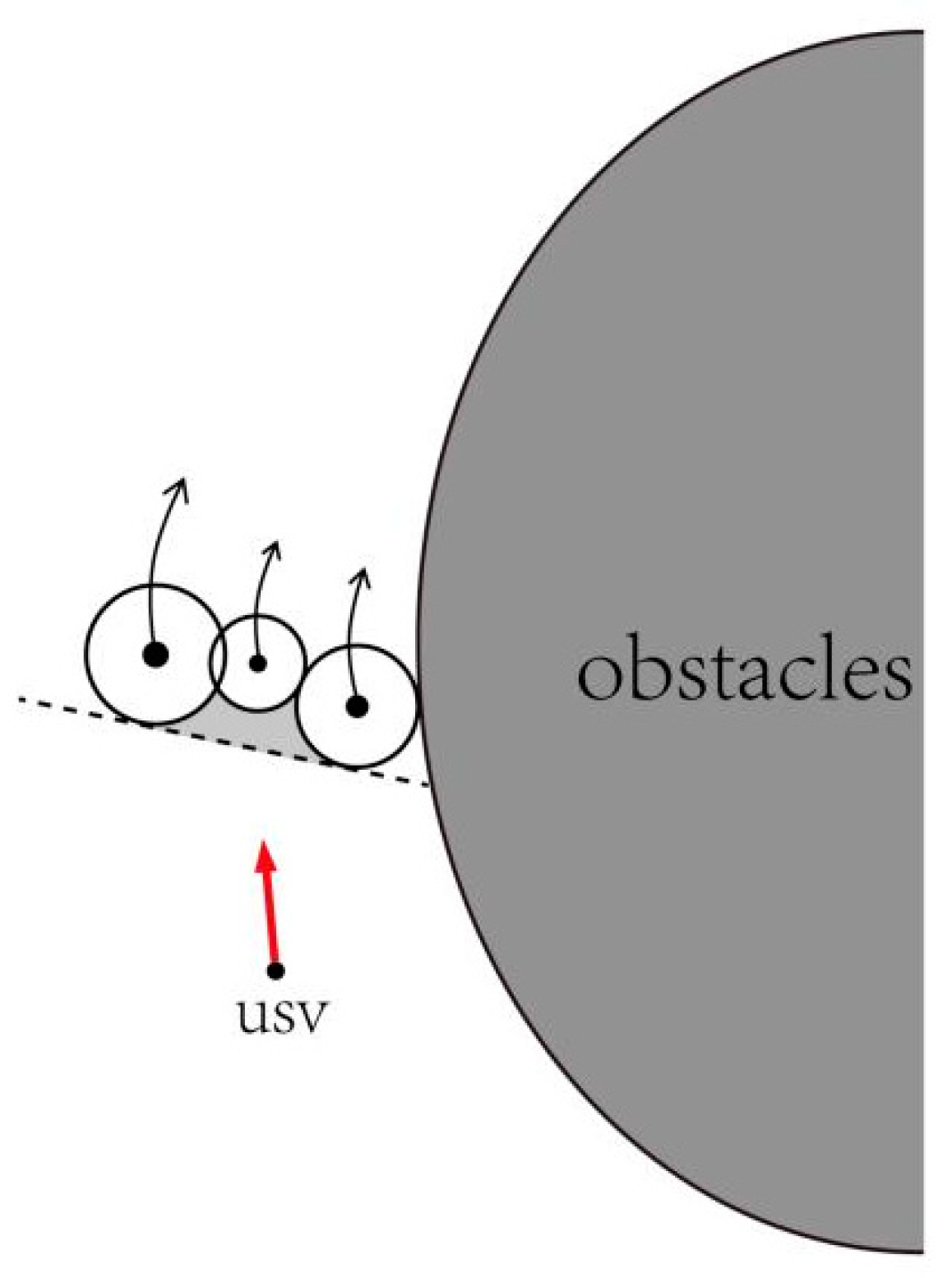
4.2. Formation Obstacle Avoidance

The formation structure, as generated by the aforementioned scheme, allows each vehicle to maintain its capability for obstacle avoidance within its respective disturbed flow field during the process of formation obstacle avoidance. Upon encountering obstacles, the formation can disassemble and later reassemble, facilitated by the traction effect of the streamlines. A significant concern addressed is the avoidance of collisions between vehicles within the formation, as illustrated in Figure 8.

As shown in Figure 8, when multiple USVs appear on the same side of an obstacle during obstacle avoidance, the streamline density on that side may become excessively high because of the contracting force within the streamlines. The streamlines do not intersect. However, as USVs are not point masses but occupy volume, they may collide with each other when the streamlines are excessively dense. As stated in Section 4.1, vehicles within the formation perceive each other as obstacles based on their hierarchy. This approach yields satisfactory results in small clusters. However, in larger clusters, the formation is already established, and too many USVs may attempt to avoid the obstacle on the same side. Consequently, some USVs may become trapped between other USVs and the obstacle, as illustrated in Figure 9. This will result in unnecessary route wastage.

To differentiate between inter-vehicle-collision and obstacle avoidance, a new approach was developed for inter-vehicle disturbances. In Equations (5) and (6), it can be shown that

$$\overline{u}=Mu=u+s.$$

(11)

Therefore,

$$\begin{array}{l}s=Mu-u\\ =(M-I)u\\ =(I-\frac{n{n}^T}{{\left|\Gamma \right|}^{1/\rho }{n}^{T}n}-I)u\\ =-\frac{n{n}^T}{{\left|\Gamma \right|}^{1/\rho }{n}^{T}n}u\end{array}$$

(12)

When $\Gamma =1$, vector $s=-\frac{n{n}^T}{n^{T}n}u$. Geometrically, $\frac{n{n}^T}{n^{T}n}u$ is the projection of $u$ onto $n$. Accordingly, an improved expression for inter-vehicle disturbance $M_j$ is proposed:

$$M_j=I-\frac{W_j{n}_j{n}_j^T}{E_j{n}_j^T{n}_j}$$

(13)

This equation gives the disturbing effect of the j-th USV on the current one, where I is the identity matrix, $n_j={\left[\begin{array}{cc}\frac{x_t-x_{jt}}{d_j}& \frac{y_t-y_{jt}}{d_j}\end{array}\right]}^T$ is the vector from the j-th USV to the current one, and $d_j$ is the distance from the current USV to the j-th one. The modulation function satisfies $E_j=\frac{\ln (d_j-D_j+\epsilon )}{\ln \epsilon }$, where $\epsilon$ is the modulation coefficient, and $D_j$ is the safety distance between vehicles.

In addition, the disturbed flow field is weighted by redefined inter-vehicle weights $W_j$ given by

$$W_j={\displaystyle {\prod }_{i=1}^N\frac{({\Gamma }_i-1)}{({\Gamma }_i-1)+e^{\eta (d_j-D_j)}}•{\displaystyle {\prod }_{jj=1,jj\ne j}^J\frac{e^{\eta (d_{jj}-D_{jj})}}{e^{\eta (d_{jj}-D_{jj})}+e^{\eta (d_j-D_j)}}}}$$

(14)

These weights are assigned to inter-vehicle disturbances, with $\eta$ being a parameter. The total inter-vehicle disturbance of the USVs is

$$\overline{M_j}={\displaystyle \prod _{j=1}^J{M}_j}$$

(15)

The total value of the initial flow field formula becomes

$$u_{jt}=\overline{M_j}{u}_t$$

(16)

Furthermore, the weight of obstacle disturbance relative to inter-vehicle disturbance is added to the inter-obstacle disturbance $M_k$:

$$M_k=I-\frac{W_{kj}{n}_k{n}_k^T}{{\left|{\Gamma }_k\right|}^{1/{\rho }_k}{n}_k^T{n}_k}+\frac{W_{kj}i{\tau }_k{n}_k^T}{{\left|{\Gamma }_k\right|}^{1/{\sigma }_k}{n}_k^T{n}_k{C}_k}$$

(17)

$$W_{kj}={\displaystyle {\prod }_{j=1}^J\frac{e^{\eta (d_j-D_j)}}{e^{\eta (d_j-D_j)}+({\Gamma }_k-1)}}$$

(18)

To verify the feasibility of the aforementioned method, the following assertions were shown to hold:

(1)

The route can reach the target point without causing inter-vehicle collisions.

Proof. 

Figure 10 presents the distance dependence of the modulation function E_j for the case $\epsilon$ = e (the base of the natural logarithms) and $D_j$ = 13 (the relative safe distance for boats in the 1-ton class is 13 m, and this distance can be adjusted for boats of different tonnages). As the distance between vehicles increases, $E_j$ gradually increases. However, the function does not converge upwards and ultimately approaches $\infty$. At this point, $-\frac{n_j{n}_j^T}{E_j{n}_j^T{n}_j}$ tends to 0, and the total disturbing effect $\overline{M_j}$ of other vehicles on the current one tends to $I$. Therefore, the total value of the flow field is $u_{jt}=u_t$. This satisfies the requirement for the route to end at the target point.

In contrast, as the distance between vehicles decreases, the modulation function $E_j$ tends toward 1. In addition, since $n_j^T{M}_j=n_j^T-\frac{n_j^T{n}_j{n}_j^T}{n_j^T{n}_j}=n_j^T-n_j^T=0$, it follows that $n_k^T\overline{u_{jt}}=0$. Thus, when the distance between vehicles equals the safety distance, the normal velocity disappears, meeting the additional requirement for the route to avoid all vehicles. □

(2)

Obstacle avoidance is given priority over inter-vehicle collision avoidance.

Proof. 

The function $e^{d_j-D_j}$ in Figure 11 gradually converges to 0 as the distance between USVs reaches the safety-distance range D_j but does not become 0. This overcomes the influence of the zero denominator in the trap area. Because $e^{d_j-D_j}$ ≠ 0, obstacle avoidance is given priority over inter-vehicle collision avoidance when a USV is on the surface of an obstacle where ${\Gamma }_k=1$. In other words, USVs can avoid obstacles without being interfered with by other USVs; the disturbance weight brought by other USVs is 0. Thus, USVs sandwiched between obstacles and other vehicles will not stagnate in the trap area or experience unnecessary oscillations in the complex disturbance environment. USVs near obstacles will always push relatively distant USVs away while effectively avoiding obstacles. Thus, the priority of obstacle avoidance over inter-vehicle-collision avoidance is satisfied. □

The proposed VST can be metaphorically understood as wrapping an outer-layer “balloon” around other USVs, as shown in Figure 12. The elasticity of the “balloon” allows USVs to avoid collisions while being pulled by streamlines. During obstacle avoidance, each vehicle follows the streamlines to evade obstacles and maintains its place in the formation because of the virtual structure law and streamlined contraction.

5. Results

This section will not elaborate on the advantages of IFDS over APF, as these have been clearly demonstrated by numerous case studies [26,27,28]. Instead, it will compare and discuss the differences between IFDS and VST.

5.1. Comparison of Local Minima Problems in Traditional IFDS and VST

VST solves the local minima problem of traditional IFDS in two dimensions.

5.1.1. Stationary-Point Problem

The stationary-point problem was simulated using the following configuration. The starting point of the USV was set to (10,10), the target point was set to (120,120), the center of the obstacle was set to (55,55), and the radius of the obstacle was set to 10 m. The velocity amplitude $V$ of the USV was set to 7.5 m/s. The results for IFDS and VST are shown in Figure 13.

In scenario (a), the disturbance coefficient ${\rho }_k$ of traditional two-dimensional IFDS was set to 3. It can be observed that the USV in the traditional approach had difficulty avoiding obstacles and tended to stagnate at the obstacle surface.

In scenarios (b) and (c), the VST disturbance coefficient ${\rho }_k$ was also set to 3 (the parameters are adjusted based on the actual usage scenario; this selection of 3 aligns better with the navigation trajectory of a 1-ton class boat. In subsequent work, we will incorporate dynamic parameters to ensure that the trajectory adheres more closely to the dynamic constraints of USV. The deviation coefficient ${\sigma }_k$ was set to 2. The parameter setting was $i=1$ in (b), and $i=-1$ in (c). It can be clearly seen that VST was not affected by the stationary-point problem of traditional IFDS in two dimensions, and parameter $i$ could be adjusted to control the USV to pass on either side of the obstacle.

5.1.2. Trap-Area Problem

For the trap-area problem, the following scenario was configured for comparison. The starting point of the USV was set to (10,10), the target point was set to (120,120); the centers of the two obstacles were set to (65,75) and (75,65), respectively; and the radius of the obstacles was set to 10 m. The velocity amplitude V of the USV was set to 10 m/s, as shown in Figure 14.

As shown in Figure 14, the disturbance coefficient ${\rho }_k$ of traditional two-dimensional IFDS was set to 3. Traditional IFDS faced the trap-area problem in two dimensions as the route passed through obstacles.

By contrast, VST could use virtual target points to effectively avoid trap areas. The VST disturbance coefficient ${\rho }_k$ was set to 3, and the deviation coefficient ${\sigma }_k$ was set to 2. It can be seen that at this velocity amplitude, VST generated virtual target points when reaching coordinates (40,40), and under the influence of these points, the USV moved away from the trap area.

5.2. VST Formation Assembly

This subsection demonstrates the application effect of VST in formation assembly. First, the initial positions of four USVs were set randomly. The initial coordinates of USV1 were (1,40), with a maximum velocity amplitude of 25 m/s. The initial coordinates of USV2 were (0,0), with a maximum velocity amplitude of 23 m/s. The initial coordinates of USV3 were (30,0), with a maximum velocity amplitude of 24 m/s. The initial coordinates of USV4 were (60,0), with a maximum velocity amplitude of 20 m/s. High-speed vehicles treated low-speed vehicles as obstacles.

The disturbance coefficient ${\rho }_k$ for obstacles was set to 3, and the deviation coefficient ${\sigma }_k$ was set to 2. The disturbance coefficient $\rho$ for low-speed vehicles was set to 1. The centers of the obstacles were located at (110,80), (40,50), (165,150), and (80,120). The radii of the obstacles were 13, 12, 11, and 10 m. The formation shape and assembly trajectories are shown in Figure 15a. The virtual formation velocity amplitude was 5 m/s.

As shown in Figure 15a, all four USVs could quickly assemble in the corresponding formation positions. Figure 15b shows that in the initial stage, USVs pursued the virtual target points at maximum velocity amplitudes; their velocities converged to those of the VSPs within a reasonable range to maintain the formation shape. Figure 15c demonstrates that there were no collisions between vehicles during assembly. Overall, VST met the requirements for formation assembly and performed excellently.

5.3. VST Formation Obstacle Avoidance

To study formation obstacle avoidance, the inter-vehicle-collision-avoidance performances of VST and IFDS were compared. A scenario was constructed in which four USVs navigated under the guidance of VSPs to avoid a nearby large obstacle. Disturbances generated by nearby large obstacles tend to make streamlines dense, which meets the requirements of the problem. The center of the obstacle was located at (90,60), and the radius of the obstacle was 30 m. The disturbance coefficient ${\rho }_k$ for the obstacle was set to 3, and the deviation coefficient ${\sigma }_k$ was set to 2. The inter-vehicle modulation coefficient $\epsilon$ was set to $e$, and the parameter $\eta$ was set to 1/5. The safe distance between vehicles was set to 12 m.

As shown in Figure 16, when avoiding a nearby large obstacle, IFDS made the streamlines too dense; it was, therefore, difficult to control the distance between vehicles. By contrast, VST had a more significant effect on controlling the distance between formation members and met the requirements of formation obstacle avoidance. Furthermore, after formation obstacle avoidance, the convergence of velocity amplitudes caused the streamlines to return to the formation shape.

6. Conclusions

We propose a new approach for obstacle avoidance and formation gathering in USV formations based on a novel VST established on the IFDS and DS methods. First, to effectively address the stagnation issue associated with IFDS when applied to USVs, a new perturbation matrix was introduced, which was validated through simulations. Second, to tackle trap zone issues, trap-area-filling and virtual target point methods were proposed, and the remarkable effectiveness of the virtual target point method was verified in simulations.

Regarding formation gathering and maintenance, based on a virtual guiding structure, USVs were tractably guided along streamlines, achieving velocity vector decoupling and the convergence of velocity amplitude to maintain formation tightness. For intra-formation collision avoidance, an innovative collision-avoidance method based on DS was employed, enhancing both the flexibility and robustness of the formation. The simulation results demonstrated that, compared to the IFDS method, VST exhibits superior performance and feasibility in obstacle avoidance and formation gathering.

In conclusion, this method provides novel theoretical support for the practical application of USV formations. However, in simulations, the establishment of the USV models did not include dynamic constraints but instead added rigid constraints, which may affect the feasibility of VST in obstacle avoidance. The future enhancements will incorporate dynamic constraints for USV based on actual usage scenarios, with a focus on optimizing adjustment parameters to meet the dynamic requirements of the USV. Drawing inspiration from the time elastic band method or employing Receding Horizon Control can further enhance the effectiveness of route optimization, ensuring practical feasibility.