Enhancing the Understanding of Subsurface Relations: Machine Learning Approaches for Well Data Analysis in the Drava Basin, Pannonian Super Basin

Abstract

The aim of this study was to confirm if predictive regression algorithms can provide reliable results in missing geophysical logging data in the western and eastern parts of the Drava Super Basin, especially Gola Field, and to apply unsupervised machine learning methods for a better understanding of lithological subsurface relations. Numerous regression models have been used for the estimation of prediction accuracy, along with some clustering algorithms to support the estimation of lithology distribution estimations in well log datasets, consisting of 20 wells in total. Tree-based algorithms and the boosting algorithm have been optimized and proven valuable in predicting well log data when they are not measured or are unavailable at all depth intervals. For blind datasets, predictions become much less reliable. For this purpose, neural networks with at least one Long Short-Term Memory (LSTM) layer have significantly improved the accuracy and reliability of predictions, not in terms of absolute values but in the aspect of the trends in values that change with the depth and other well features, as well as in terms of the magnitudes. Trendlines can further be used for pattern recognition or as a newly engineered feature. Unsupervised learning has confirmed reliability in lithology recognition on validation sets and has proven to be a great asset in distinguishing variabilities in the petrophysical properties of sediments.

1. Introduction

Well logging data is essential for the characterization of subsurface relations. This includes the petrophysical properties of the subsurface and the correlation between the elastic properties of rocks and the lithology, i.e., the calibration of reflection seismic data with well data. Even though petrophysical properties include a variety of rock properties that are related to pore distribution and fluid behavior within the rock, such as mineralogy, porosity, capillarity, and fluid saturation [1,2], in the context of this paper we are mainly referring to porosity and permeability [3]. Unfortunately, different sets of well logs are not always available. This is a result of either the specific measurements not being measured in a well, measured only in a certain well interval, or of poor quality in some cases, even if they are measured, due to the well conditions. All of the above is also the case in the Croatian part of the Drava Basin, the area of research further discussed in this paper. Furthermore, the area of research contains parts of the eastern and western Drava Basin, and even though the Pannonian Basin has been extensively researched, the area in question is characterized by a complex alteration of sandstones and shales. The uniqueness lies in several channel sandstone bodies within a progradational system that has taken part during the Neogene, which has led to the formation of lenticular sandstone bodies. Even though permeable deposits are relatively easy to distinguish on well logs, intrications can arise due to their shape, dimension, and dynamic intertwining with impermeable rocks. When the well data are sparse in usability, other methods are helpful for the further analysis and processing of the available data. In this case, machine learning methods are relatively inexpensive methods, even though they charge in terms of time. The application of machine learning (ML) methods to well log analysis and petrophysics has grown rapidly from the 2010s to the present day [4,5]. Statistical techniques, along with supervised and unsupervised machine learning algorithms, have been successfully applied to well logs for lithofacies identification [6,7,8] and reservoir characterization [9,10,11]. A machine learning model for lithology prediction depends on the quality and representativeness of the input data, and the suitability of the chosen algorithm.

The main object of this research was the application of machine learning algorithms within the Neogene-Quaternary infill in the Drava Basin. The focus of this research was the Gola Field locality (Figure 1), as the data from production wells contained a large geophysical dataset suitable for machine learning training. The goal was to find alternative ways for well data preparation and interpretation to come to an uplifted lithological characterization and a better understanding of the spatial position of the sandstone bodies. From the available well data, a prediction of missing log data, especially the acoustic log, has been made. Based on the relationship between various well logs, such as resistivity logs and gamma-ray logs, spontaneous potential, calipers, and missing logging intervals of interest were recreated. Since the Gola Field dataset in western Drava contains a large amount of information, this location was the focal point of this study. Recreating and analyzing data there helped with extrapolating the methodology on the wider area of eastern Drava. Besides recreating data for an increase in interpretation materials, clustering analyses were used for the recognition of lithology patterns in well logs. Exploratory Data Analysis (EDA), as well as regression and clustering models, were carried out using the Python programming language.

In addition to lithological grouping and reservoir rock typing, the application of machine learning includes a prediction of continuous petrophysical properties from core data [12,13] and a prediction of missing well log data [14,15].

In the Croatian part of the Pannonian Basin, several researchers have successfully applied Artificial Neural Networks (ANNs) for lithology prediction based on seismic attributes and well log data. For instance, refs. [16,17,18] applied ANNs in the Sava Basin (Croatia, Figure 1) for a prediction of lithology and hydrocarbon saturation. The authors of ref. [19] demonstrated the efficiency of ANNs for lithofacies modeling in Požega Valley, Sava Basin, based on limited well data and 2D seismic reflection data, while [20] applied an ANN for the lithology prediction of clastic sediments in the eastern part of the Drava Basin. However, there are very few studies in the Croatian part of the Pannonian Basin that apply machine learning algorithms for lithology prediction or classification. For example, ref. [21] applied the XGBoost algorithm for lithology classification in the Serbian part of the Pannonian Basin based on well logs, core data, and depositional environment information.

In Gola Field, which is in the western part of the Drava Basin, 17 machine learning algorithms were tested and used for predictions on log data and five were used for unsupervised learning regarding lithological determination in order to clarify the subsurface relations in the area and apply the most suitable methods on the eastern Drava Basin dataset.

2. Geological Background

The Drava Basin is an elongated WNW-ESE trending, tectonically subsided basin with a maximum thickness of Neogene and Quaternary sediments of about 7000 m [22,23]. Lithostratigraphic division for the western part of the Drava Basin corresponds to the one in the Sava Basin due to similar depositional processes [24], while it is somewhat different in the eastern part of the basin.

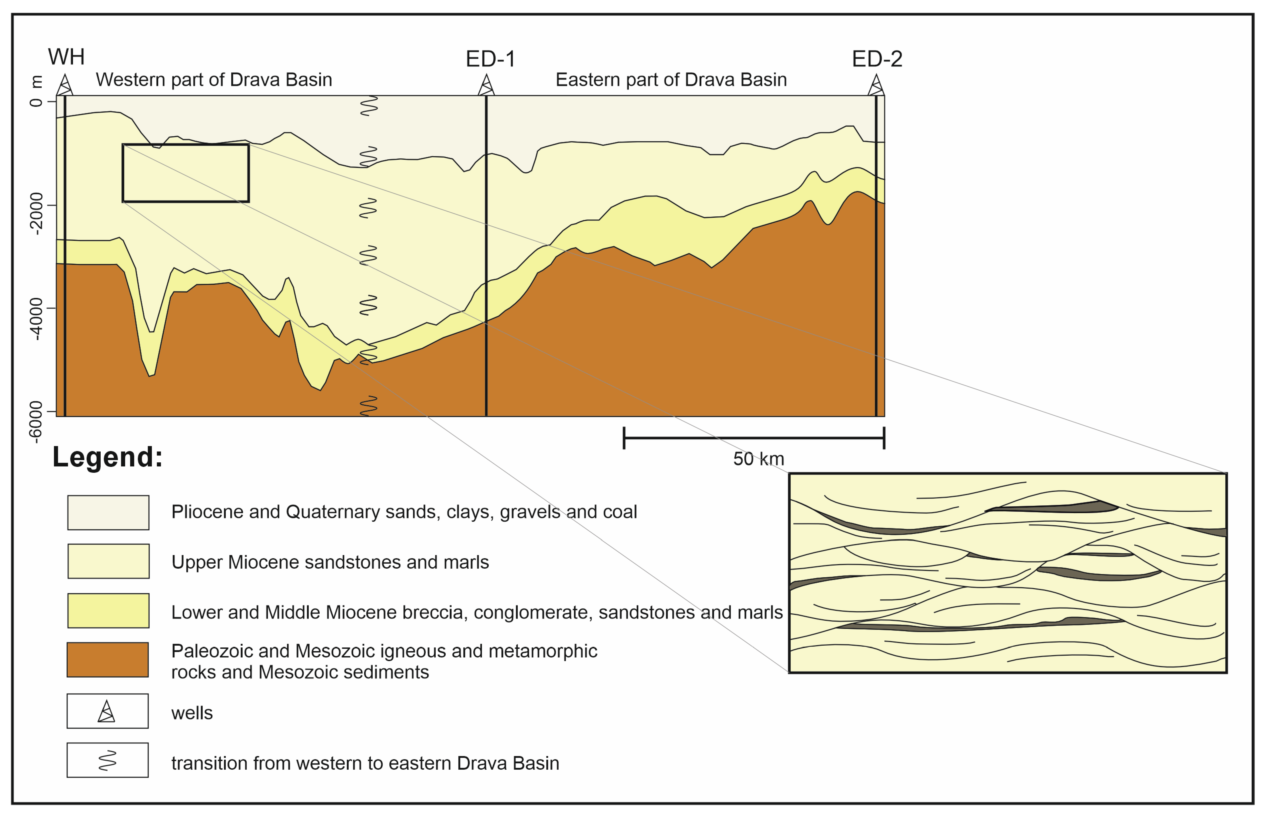
According to [22,25], the Neogene sedimentary sequences in the western part of the Drava Basin were formed during three depositional megacycles. The first megacycle started during the Early Miocene and is composed of Lower to Middle Miocene syn-rift and early post-rift sediments. Terrestrial sandstones, coastal breccias, conglomerates, and sandstones were deposited, and they are overlain by shallow to deep marine marls and shales with thin sandy intercalations, while biogenic and bioclastic limestones were deposited in the coastal zone [26] (Figure 2). The end of the megacycle is characterized by the deposition of fine-grained sediments in the brackish water basin. The Sarmatian/Pannonian boundary is marked by decreased salinity and the sediments of a brackish water environment [27]. The second megacycle is associated with the thermal subsidence of the Pannonian Basin during the Late Miocene. The sedimentary sequence begins with littoral limestones and a nearshore transgressive layer overlain by hemipelagic calcareous and clayey marls [27]. The western part of the Drava Basin was filled to lake level and the youngest deposits of this megacycle were formed in fluvial environments. In the eastern part of the Drava Basin, deposition continued on the delta front [28,29]. The third megacycle lasted from the Pliocene to the Quaternary and was characterized by the shallowing of the large lake environment and the transition to marsh and then terrestrial environments [27,30], accompanied by a compressional type of tectonics [25].

In the western part of the Drava Basin, the main hydrocarbon reservoirs are located within conglomerates and sandstones of the Lower and Middle Miocene (first megacycle) and Lower Pannonian sandstones (lower part of the second megacycle). However, Upper Pannonian sandstones also have good reservoir properties [22].

The main target of this research is the Upper Miocene sediments of the Gola Field, located in the southwestern Pannonian Basin near the Croatian–Hungarian border and the Drava River (Figure 1). The Neogene sediments represent important reservoir rocks and form a sequence of sandstone, siltstone, marl, and their transitional lithofacies due to the depositional conditions in this area. These deposits were formed in a brackish lake environment in the zone of the lake littoral and part of the sublittoral and represent sediments of channel fill and underwater delta, deposited by turbidites [31].

They mostly occur in lenticular forms, which makes their accurate identification and spatial correlation challenging [31]. The problem is particularly emphasized when there is a lack of well logging data. Any approach to estimating lithology, such as geophysical modeling, the application of various statistical methods, or artificial intelligence methods, would provide more reliable results if the input data are consistent and complete.

3. Materials and Methods

The dataset consisted of well log data from ten wells within Gola Field, from the western part of the Drava Basin, and ten wells from the eastern part of the Drava Basin. Although a large number of logging measurements have been performed, it is important for machine learning purposes to distinguish which data can be used in regard to the quality and completeness of the dataset (Link in Supplementary Materials: Exploratory Data Analysis). Density logs, acoustic and neutron logs, calipers, spontaneous potential, gamma rays, and various shallow and deep resistivity log measurements were available in most of the wells, with a sampling interval of 0.1 m.

Machine learning (ML) is a method of data analysis that uses algorithms to recognize patterns present in the data. It assumes that systems can learn from data and the learning process is improved without having to be explicitly programmed [4,32]. The drawback of the method is the data preparation process for ML algorithm applications, as it is time-consuming. Even though the structure of logging data remains the same no matter the contractor, log names and acronyms may vary. In addition, there are very often duplicate measurements for particular logs that need to be thoroughly compared and the reasoning behind them needs to be validated. Along with raw measurements, there are oftentimes corrections and additional analyses being generated from raw data that need to be examined particularly carefully, in terms of understanding the background behind their making [5,33]. Even after the exploratory data analysis has been performed, the model building based on the cleared data can shed a different light on the input data being used based on the type of algorithm that is being used and its hyperparameters [34]. To obtain the best results from the learning process, analysis of outliers could be very helpful, as well as normalization and standardization [35]. However, once the machine learning model is built, it can be fed with input data and used for its intended purposes. In the current research, multiple well-known regression models have been used to find the best models for predicting our data, especially acoustic well logs (AC). They belong to supervised learning models, which means that the test data consist of different input variables and the target variable represents the desired output of the learning process [9,14,34,36,37] (Links in Supplementary Materials: Supervised learning). Unsupervised machine learning algorithms have also been used to gain a better understanding of the spatial distribution of the Neogene sediments in the researched area [8,38].

In this study, machine learning techniques were applied for predicting well logs to see if the models can be reused on different parts of the Drava Basin and in which cases (Figure 3). The measured values of well logs have been further analyzed alongside the predicted values to recognize similar patterns in the whole dataset that would reflect the lithology distribution. Since the lithology in this case was treated as an unknown variable, unsupervised learning was applied, more specifically clustering algorithms.

All of the data analyses and processing have been performed using the Python programming language, and the exact packages are disclosed further in the subsections.

3.1. Exploratory Data Analysis (EDA)

The first step was to visualize the available data and check for completeness of the available data, where completeness represents the percentage of all the available logs being measured at the same interval. Analyses revealed that some of the logs were measured only in a small depth interval related to the targeted hydrocarbon accumulation or only in a single well. Out of the ten wells in Gola Field, acoustic logs were measured entirely throughout the well in only three wells, while they were either partially measured or not measured at all in the other wells of eastern and western Drava. The acoustic log was predicted after successful training of the models using neutron logs, density, gamma rays, spontaneous potential, and resistivity logs. A caliper log was used for outlier removal caused by the rugosity of the well prior to the training process.

Although collecting as much data as possible is essential for the statistically favorable performance of the machine learning model, the algorithmic processing of a large amount of data is only possible if the input data matrix is not singular, i.e., if its determinant is not zero. The problem is that most logging data sets are in the form of a singular matrix, since most wells lack values at certain depth intervals [39]. Therefore, to make the input data set reliable for testing the algorithms, some of the valuable data had to be removed from the dataset. Afterwards, outlier analyses were performed on the data, but since the statistical outliers could have geological meaning, especially if natural gas can be recognized on the logs, only very extreme values have been removed.

Each measured geophysical parameter used to build the predictive model represents a single variable of the model, and the range of values of these variables varies greatly (depending on the measured physical parameter). For this reason, preprocessing of the input data is required, and the data must be standardized, normalized, or transformed, depending on the algorithm used. All transformations in this study were performed using the scikit-learn package [40] and the pandas [41,42] and NumPy [43] libraries, after the logging data were analyzed with a lasio library [44].

3.2. Regression Models for Well Log Prediction

As well logs are a visual representation of numerical data for a well interval, regression prediction models were selected for the prediction of the AC log. In accordance with the correlation matrix of the available logs, nine were selected for the training of the machine learning model. As many of the machine learning algorithms cannot be used with categorical variables, One-Hot Encoding was used to transform well names. After including the names and spatial coordinates of wells, 14 features in total were available for building models. The entire dataset is first divided into a training set (learning set) and a model testing set. To evaluate the accuracy of the trained model, the learning set is further divided into a model validation set. This avoids the bias of a model that would be built on only part of the data. For this purpose, K-Means validation was used to ensure that each data point in the learning process was part of the learning set and part of the validation set. Of the total number of values that each variable can take, 30% were used to test the model. A total of 17 regression models were used to predict the acoustic log. The base models were built using a sci-kit learn python package with default hyperparameters [40] (

Table 1. Regression models tested for well log prediction and their results on test data from Gola Field (the table primarily shows the results of acoustic log prediction).

	ML Models (Default Hyperparameters)
	ET	RF	XGB	DT	KNN	LGB	MLP	GB	SVR	AB	RIDGE	KR	LR	LASSO	PLS	ELNT
RMSE	1.61	1.95	2.64	2.77	2.81	3.44	4.08	4.13	4.66	6.51	7.88	7.88	7.88	8.80	10.17	10.83
R2	1.00	1.00	0.99	0.99	0.99	0.99	0.98	0.98	0.98	0.96	0.94	0.94	0.94	0.92	0.89	0.88

).

After the learning process, the accuracy of the algorithm was evaluated (Figure 4). The most common regression performance metrics are the Mean Absolute Error (MAE), the Mean Squared Error (MSE), the Root Mean Squared Error (RMSE), and the coefficient of determination R². The performance metrics were calculated according to formulae described in [45], where $X_i$ represents the predicted $i^{th}$ value, and $Y_i$ is the actual, measured $i^{th}$ value. The regression models predict the $X_i$ element of the corresponding $Y_i$ element in the measured data.

Each of these parameters has its advantages. MAE is given in the units of the variable values:

$$MAE=\frac{1}{m}{\sum }_{i=1}^m\left|X_i-Y_i\right|,$$

(1)

MSE is used to calculate the loss function:

$$MSE=\frac{1}{m}{\sum }_{i=1}^m{(X_i-Y_i)}^2,$$

(2)

RMSE is used to calculate the learning curve:

$$RMSE=\sqrt{\frac{1}{m}{\sum }_{i=1}^m{(X_i-Y_i)}^2},$$

(3)

The highest score for MAE, MSE, and RMSE is 0, and the lowest score is +∞.

R² is used for the indirect assessment of the reliability of predictions (shows how well the regression line describes the data):

$$R^2=1-\frac{\sum _{i=1}^m{(X_i-Y_i)}^2}{\sum _{i=1}^m{(\overline{Y}-Y_i)}^2},$$

(4)

where the best score is +1 and the worst score is—∞.

3.3. Clustering Models for Lithology Prediction

Spatial grouping, known as Clustering, includes methods for unsupervised machine learning. This means that patterns and connections are sought within the data set that are not clearly visible, i.e., the patterns are not known in advance and it is left to the algorithms to recognize them. Data are grouped into clusters based on their relationship with the surrounding data (Link in Supplementary Materials: Unsupervised learning). In the end, groups are made up of elements with similar or the same characteristics. The principle of grouping non-hierarchical models can be based on the density of data in a certain area, on the distribution of data, or data added to centroids. For the clustering of eastern and western Drava Basin datasets, a few of the clustering algorithms have been tested, such as K-Means on standardized and Principal Component Analysis (PCA) reduced data, the Gaussian Mixture Method, Spectral Clustering, Agglomerative Clustering, and Mean Shift (Figure 5). Well log data have been divided into an optimal number of clusters based on specific curve patterns (Figure 5). The dataset on which the clustering was performed is the same dataset used for training supervised prediction models. The difference is that for the clusters to be generated, models do not need to be presented with the output lithologies. However, to verify results, the lithologies in terms of sandstone bodies and shale deposits have been conventionally interpreted using the well logs, and nine different sandstone bodies have been recognized throughout all the wells (Figure 6).

As an additional feature of comparison, the volume of shale has been calculated using the following formula:

$$Vs{h}_{calculated}=\frac{G{R}_{measured}-G{R}_{minimum}}{G{R}_{maximum}-G{R}_{minimum}}$$

(5)

Intervals for calculating the volume of shale (Vsh_calculated) have been restricted to intervals used for machine learning training data and those are the intervals with measured gamma ray responses (GR_measured) (Link in Supplementary Materials: Petrophysical calculations). The lowest gamma ray log values are associated with the lowest shale concentrations, and vice versa.

4. Results

Baseline regression models for each algorithm were tested on the blind dataset that has never been in a training set. Even though an unseen dataset comes from a well from the same exploitation field, its position is the furthest from most of the training wells.

After the base model estimations, regression models were trained by optimizing the model parameters (Links in Supplementary Materials: Hyperparameters tuning), i.e., the parameters within the model were searched for those that yielded the best coefficients of determination and the smallest root mean squared errors. By achieving this, the probability of obtaining a prediction with minimal deviation from the real data is the highest.

GridSearchCV and Bayesian optimization were used for further hyperparameter tuning, as previously performed in [34] (

Table 2. Selection of regression models that have been optimized for well log predictions, including an LSTM neural network that is specialized in sequential data (the lowest scoring models were not further tuned).

	ML Models (Tuned Hyperparameters)
	ET	RF	XGB	DT	KNN	LGB	GB	SVR	AB	LSTM	RIDGE	PLS	ELNT
RMSE	1.57	1.93	1.69	2.71	2.29	2.52	1.66	3.84	5.90	3.16	7.88	7.88	7.88
R2	1.00	1.00	1.00	0.99	0.99	0.99	1.00	0.98	0.96	0.96	0.94	0.94	0.94

). It can be observed that optimization has been the most beneficial for underachieving algorithms; however, overall, the highest-scoring algorithms before the procedure performed better even without hyperparameter tuning.

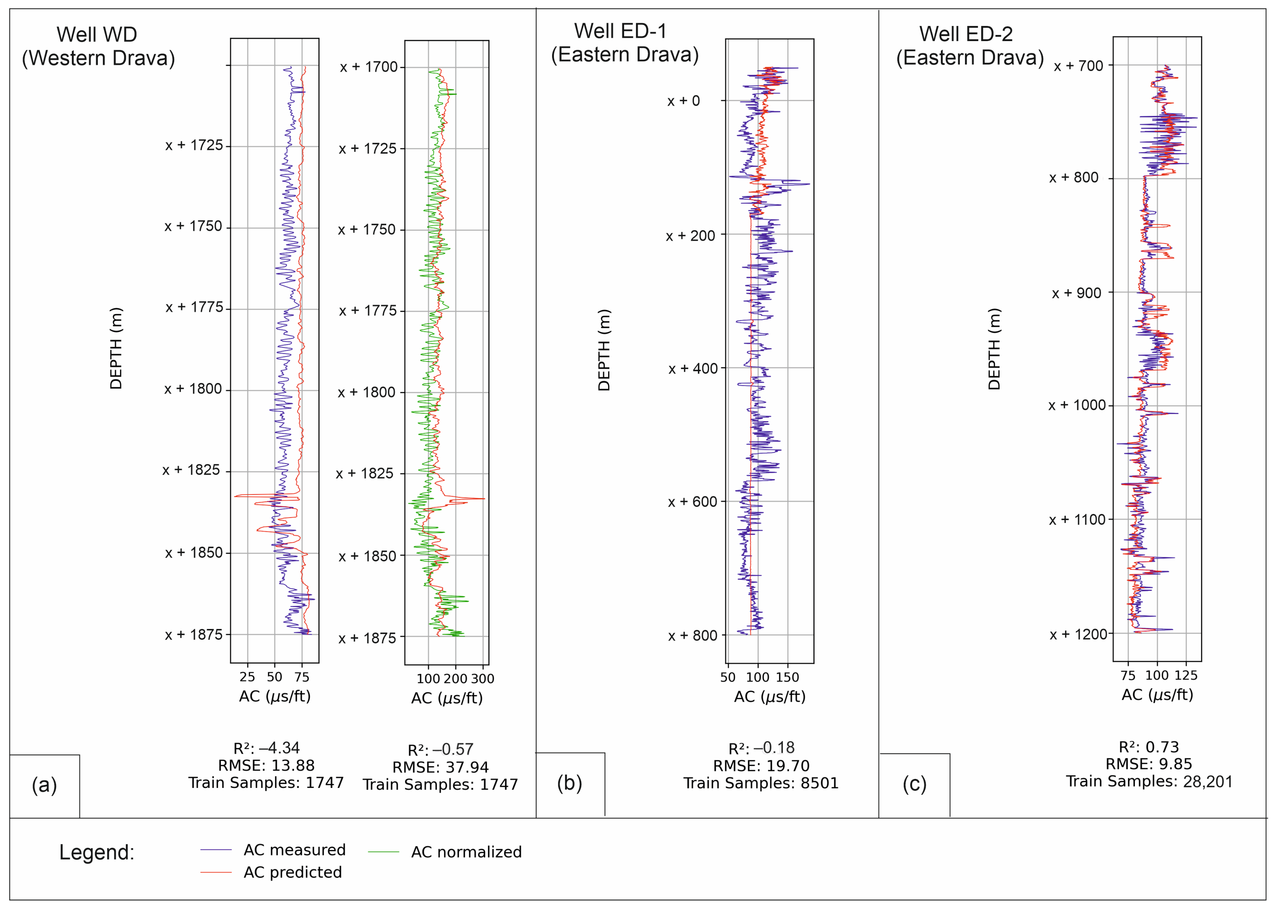
Even with the great prediction of sonic logs on the Test Dataset (R² over 95%), the most successful algorithms were struggling with the unseen data and even the five best algorithms had issues with predicting stable results. However, the only model that showed improvement with unseen data was the artificial neural network. With two hidden layers of 150 and 50 neurons, the tanh activation function, and the lowest learning rate of 0.00001, it was possible to achieve a 0.73 coefficient of determination (Figure 3). With negative coefficient values for all the other algorithms, the neural network was the only one that was able to recognize the data trend on unseen data. The best neural networks for reliable trend predictions on the well data were the ones with the added Long Short-Term Memory (LSTM) layer, which has also been explained in previous papers [46]. It was interesting to observe variability in the ability of the LSTM model to reliably predict well log values across the wells in both the western and eastern parts of the Drava Basin. Even though the model itself was trained and optimized solely on the data available from the western Drava Basin, and even more locally on data from Gola Field, it showed some of the highest results of prediction (coefficient of determination, R²) on the wells in the middle of the eastern Drava Basin (ED-2) (Figure 3). On the other hand, wells that are the furthest East (ED-1), almost on the border with the Republic of Serbia, showcased the worst results of prediction in the entire blind dataset (Figure 3). Since the well logs available from the eastern part of the Drava Basin were not included in the training dataset for model building, the result shows a step forward into a more generalized machine learning model that would be applicable in a much wider, lithologically complex area of the Drava Basin. The wells from eastern Drava were purposefully excluded from the training dataset as the scarcity of some of the log curves that were determined to be the best for model building was the higher of the two sets. Furthermore, the year of well completion made a large contribution to the decision for selecting data, as a large portion of the wells were drilled over three decades ago. This means that most of them were vectorized throughout the years and the log values have a higher chance of being contaminated by an error. However, based on the varying values of prediction results, a model trained in different parts of the basin can provide a lot of information about the similarity of the subsurface in eastern and western areas. Higher values of the coefficient of determination show that the middle-eastern Drava shares similar petrophysical subsurface properties to the western Drava Neogene deposits (Figure 3c). The low or negative values of the coefficient of determination represent wells in the parts of eastern Drava where petrophysically different sandstones are expected, or in variable abundances alongside their lithological similarity (Figure 2). While the wells positionally furthest from the research area in focus (western Drava) were expected to show the highest correlation between the measured and predicted well logs, this was not the case here (Figure 3a). The results contribute to the fact that the Gola Field area has a lot of variations in properties of seemingly simple lithology (mostly sandstones and shales). The LSTM model was built using the TensorFlow platform [47].

The variations in properties are indicative of the structure of the input data for the model needed. The more geologically complex the region, the more well data is needed to establish the relations of petrophysical and lithological properties, which is why the trained LSTM model competently handles missing values in the wells that have been part of the learning process (Figure 4). Primarily, the training dataset consisted of the measured intervals where all the input variables were present. Therefore, even if there were ten wells with measured data for training to begin with, in the end, all the prediction models had to be built on five partial wells, which is why the results of predicting the missing values of acoustic logs (AC), density logs (DEN), and compensated neutron logs (CN) show higher RMS errors for wells with less available data (Figure 4). However, the predicted values are highly correlated to the measured values, and with R² values between 0.52 and 0.98, tuned LSTM architecture has been proven to be able to efficiently predict the missing intervals of AC, DEN, and CN well logs in Gola Field test data (Figure 4). This is why it is a great tool for predicting well logs, specifically AC, DEN, and CN, in wells that do not have these measurements (Figure 4).

When it comes to clustering methods, only well WH contained applicable data throughout the whole well, which is why it was used for presenting the results. The interval of interest consisted of Neogene sediments that were easily distinguished by using the statistically optimal number of clusters. The optimal number was defined with the silhouette method which resulted in five clusters. One of the five clusters (golden-brown) was correctly assigned to Pliocene deposits and the remaining four were assigned to values corresponding to sandstones and shales (Figure 5). Based on the a priori interpreted sandstone bodies, it is visible that all the values assigned to sandstone clusters (yellow and red) are correctly assigned. However, some of the sandstone bodies were still wider in range than interpreted. The thicker sandstone body patterns were easily recognized by algorithms, including in the shallower interval (2000–2200 m), while the deepest sandstone body was not fully recognized (Figure 5). For this reason, additional clusters have been added to deepen the interpretation.

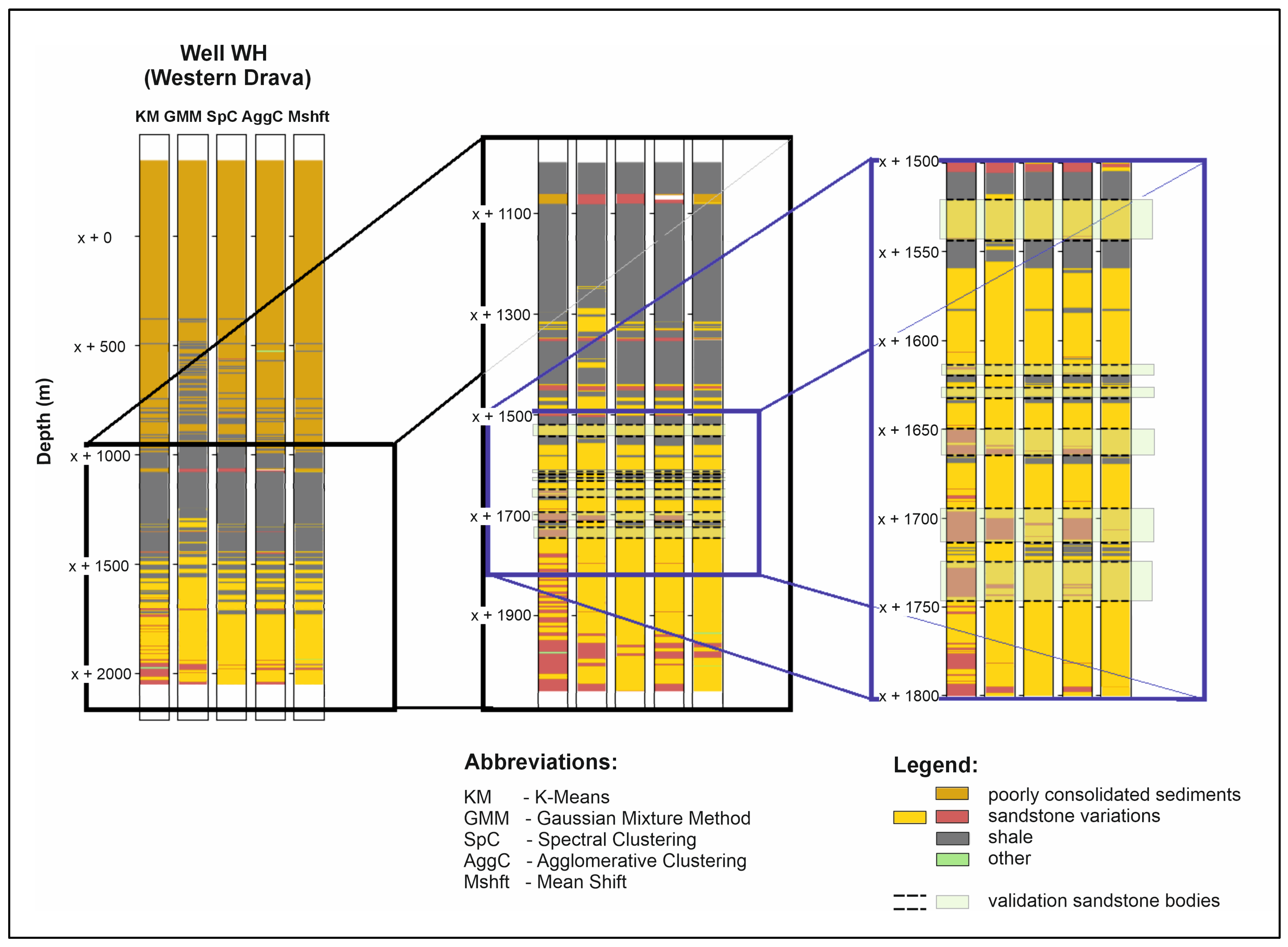
After increasing the number of clusters from five to six and ten, differences in the properties of sandstones became more emphasized. However, the alteration of lithology in Pliocene deposits was even more emphasized and after excluding the younger interval, six recognizable clusters remained (Figure 6). Based on the resolution of data and data interpreted for verification, there was no need to introduce new clusters (Link in Supplementary Materials: Cluster label matching). Even though the higher number was tested as well, it provided no additional information about the data that can be verified.

It is interesting to notice that four variations of sandstone properties have been recognized. Different clusters represent sandstone bodies of different petrophysical properties. What is also noticeable is that all the validation sandstones are a combination of blue clusters, with other clusters defined as sandstone by the majority of algorithms and confirmed by logging data. Blue clusters represent bodies with lower gamma ray, density, compensated neutron, and spontaneous potential log values (GR, DEN, CN, and SPT), as well as higher resistivities (RT) (Figure 7). As the blue cluster has been correlated with higher resistivities and is mostly recognized in the top parts of the identified sandstones, there is a possible relation to gas-bearing reservoirs. In addition, a crossover of the log curves is observable on the CN-DEN plot at some of the intervals, which could aid the interpretation [48] (Figure 7).

5. Discussion and Conclusions

The prediction of well logs, specifically an acoustic log with regression machine learning algorithms, has shown great results on the test datasets. All 17 of the tested algorithms have predicted acoustic log values with over 80% correlation between the originally measured and predicted data. The highest scoring algorithms are tree-based structured algorithms (DT, RF, and ET), boosting algorithms (GB, XGB, and LGB), and neural networks (MLP and LSTM), with over 90% correlation between the predicted and original values. The results of the predictions of acoustic logs on blind data have been lower, with measured and predicted target variables showing up to 75% correlation at best but with distinguishable trendlines to the actual measured data.

By using regression learning models, it is possible to precisely determine individual logging curves if the training dataset is large enough to represent parts of lithologically similar data. This can be useful in predicting missing parts of well logs for which there are other well logs available. The accuracy of correctly predicting well log values depends on the curve being predicted and its correlation to the feature values, as well as on the spatial location of the well itself. The correlation between measured acoustic logs and predicted logs has been astonishingly high for the tested data and validation data. The values can be predicted with a correlation of up to over 95%. When it comes to blind wells, or unseen well data, a neural network has proven to be the best scoring algorithm and has been able to achieve correlations between the measured and predicted well data of up to 45% for acoustic values, but it depends on the curve being predicted. Nevertheless, the neural network, especially the Long Short-Time Memory (LSTM) layered network, has shown great predictions of measured trendlines. The trendlines could provide great insight into subsurface patterns and relations. Furthermore, some of the predictions with the highest correlation in blind wells are proven to be the ones from the eastern part of the Drava Basin. Despite the complexity of the lithological distribution in the subsurface, the LSTM model has given excellent results in predicting missing well log data in wells that have been trained on and can provide a good starting point for the interpretation of regional subsurface relations in the area. The starting point would mean that petrophysical similarity can be estimated between the deposits of different parts of the Drava Basin based on the reliability of the prediction models.

When it comes to lithology prediction using unsupervised clustering algorithms, these were tested for five to twelve clusters. The lowest number of clusters has been defined as optimal by different statistical methods, and the higher number of clusters has been recognized to be more accurate in representing lithological patterns. The optimal number of clusters has been calculated to be five and was sufficient to enable recognition of the interval of interest, i.e., the Neogene sediments, as well as the permeable and impermeable deposits, sandstone, and shale. By adding new clusters, more variations in these deposits could be noticed. For this purpose, ten clusters were the optimal number for the validation of sandstone bodies. There was one specific cluster, categorized in blue in this case, that was identified inside all the verified sandstone bodies and could be correlated to gas-bearing reservoirs.

All of the used algorithms have given similar results of grouped data that can be correlated to lithological properties. The Gaussian Mixture Method and Spectral Clustering have more effectively captured the variations of clusters in a dataset. Depth intervals with fewer data were still prone to be assigned to a less accurate lithology representative or a thicker interval.