One Method for Predicting Satellite Communication Terminal Service Demands Based on Artificial Intelligence Algorithms

Abstract

This paper presents a traffic demand prediction method based on deep learning algorithms, aiming to address the dynamic traffic demands in satellite communication and enhance resource management efficiency. Integrating Seq2Seq and LSTM networks, the method improves prediction accuracy and applicability, especially for mobile terminals such as aviation and maritime ones. Unlike traditional approaches, it does not require extensive statistical data and can be generalized to real-world systems, providing stable long-term traffic demand predictions. This study utilizes real-world flight data mapped to corresponding satellite beams, allowing the precise prediction of beam-specific traffic demands. The results show that aggregating historical demand data for beams with similar trends achieves an average predictive Mean Squared Error (MSE) of 0.0007 and a maximum MSE fluctuation of 0.014, significantly outperforming predictions based on average values in terms of stability and accuracy. This novel solution for resource management in satellite communication ensures efficient and accurate long-term traffic demand predictions.

1. Introduction

The next-generation broadband communication satellites will achieve throughput rates of several gigabits per second or terabits per second (Tbps), with the number of beams increasing from dozens to hundreds. With the proliferation of mobile terminals such as airborne, maritime, and high-speed rail terminals, communication satellites face challenges such as an uneven distribution of user geographic locations and tidal effects and varying business hour demands. Traditional communication satellites often encounter situations where beams cannot meet demands, leading to resource wastage.

The application of flexible payloads underscores the importance of predicting related traffic demands. In a flexible communication satellite resource management system, resource prediction serves as input for resource management. By forecasting future traffic demands based on past demand patterns, resource utilization efficiency can be improved, aiming to achieve effective resource management [1].

In study [2], the authors discuss that the demand for each beam in a satellite communication system is primarily influenced by factors like population density in service areas. They propose a traffic demand prediction model that relies on specific population parameters to estimate these demands. The model defines key factors such as the throughput per user, population density, penetration rate, and concurrency rate. These parameters are used to calculate the expected traffic demand within a given area.

The authors propose that the total traffic demand for each beam is determined by the product of the beam area and the average traffic demand per unit area. They define a function to compute the average traffic demand based on throughput per user, population density, and other relevant parameters. While this model offers a framework for estimating traffic demands, it has notable limitations. It requires extensive statistical data on population characteristics specific to different regions, making it highly dependent on large-scale empirical measurements. This reliance on detailed regional data limits its generalizability to areas with differing demographic and geographic characteristics. Furthermore, the model focuses on short-term capacity predictions, which restricts its utility for proactive and long-term resource management. Similarly, in their research on the satellite traffic demand, scholars Z. Lin et al. derived the total traffic demand for each unit based on the global population distribution. In addition to the aforementioned shortcomings, neither approach takes into account the mobile terminals in aviation and maritime sectors [3].

In study [4], a deep learning Convolutional Neural Network (CNN)-based architecture is proposed to predict significant rain-fade in satellite communication using satellite and radar image data, as well as link power measurements. For better understanding, a CNN is a type of neural network specifically designed for deep learning. It learns directly from data using convolutional layers that help detect patterns and relevant features in the input data, such as images. By processing data through multiple layers of convolutions, a CNN can identify complex patterns and extract significant features that are crucial for tasks like image recognition, object detection, and, in this case, predicting rain-fade for the next hour using satellite images from the past 30 min. To capture the spatiotemporal dependencies between satellite and radar images, the authors selected a three-dimensional Convolutional Neural Network (3D CNN) as the core component of their baseline architecture. To validate the effectiveness of the 3D CNN in this context, they employed accuracy and the F1-score as key metrics for model evaluation. Accuracy measures the overall proportion of correctly classified instances, while the F1-score balances precision and recall, providing a more nuanced assessment of the model’s performance, particularly in imbalanced datasets. These metrics were chosen to comprehensively evaluate the model’s ability to handle both spatial and temporal data. While the 3D CNN is capable of learning temporal relationships between input images across different time steps, it primarily focuses on extracting spatial features. This limitation restricts its effectiveness in predicting long sequences with significant temporal characteristics. As a result, the authors’ model is only capable of making accurate predictions for up to 60 min. This constraint arises because the 3D CNN is inherently designed to capture spatial patterns rather than long-term temporal dynamics, making it less suitable for extended period predictions and limiting its utility in scenarios requiring longer-term forecasting. In the prediction of communication satellite traffic demands, traditional methods have two significant drawbacks:

(1)

In current communication satellite traffic demand prediction, large-scale statistical measurements of population characteristics in specific regions are required, without considering the prediction of needs for mobile terminals such as aviation and maritime ones, making it difficult to generalize to real systems [2,3].

(2)

In current communication satellite traffic demand prediction, the focus is mainly on predicting short-term traffic demands, with poor performance in long-term prediction [4].

Usually, time series prediction involves forecasting the observation value for the next time step, known as “single-step prediction”, as only one time step is predicted at a time. However, for more complex time series problems, predicting multiple future time steps is often necessary, referred to as “multi-step time series prediction”. The essence of demand prediction for satellite communication fundamentally requires a multi-step time series approach. This is the primary basis for proposing our model, which aims to overcome the limitations of single-step predictions. Unlike single-step prediction, which forecasts only the immediate next step, multi-step prediction provides a more comprehensive view of future demand, enabling better resource allocation and management in satellite communication. By incorporating multiple time steps into the prediction process, our model addresses the dynamic nature of satellite traffic and improves the accuracy and robustness of demand forecasting. Multi-step prediction models are particularly useful in satellite communication algorithms as they facilitate proactive planning and more effective management of varying traffic demands over time. Additionally, by predicting future traffic trends, multi-step models allow for the proactive allocation of satellite beams, thereby improving user satisfaction through better resource availability and service quality.

The field of time series prediction has long been influenced by linear statistical methods such as ARIMA models. However, in the late 1970s and early 1980s, it became increasingly clear that linear models were inadequate for many practical applications [5]. Over the past twenty years, the rise in artificial intelligence has brought machine learning models into view and has become a powerful competitor to classic models in the prediction field [6]. Artificial neural networks (ANNs) are one of the widely used machine learning techniques for time series prediction. ANNs provide linear and nonlinear modeling without assuming the relationship between input and output variables. Therefore, artificial neural networks are more flexible and applicable than other methods [7].

There are various strategies such as direct prediction, recursive prediction, direct recursive fusion prediction, multiple output prediction, Seq2Seq, etc., to address multi-step advance prediction tasks. These underlying model strategies can be applied to almost any prediction model [8]. Teams like An’s and scholars like Taieb compared three methods, direct prediction, recursive prediction, and fusion prediction, and found that fusion prediction is always superior to or at least comparable with the best strategy among recursive and direct strategies. It avoids the difficult task of choosing between recursive and direct strategies, making it more competitive than these two strategies [9,10]. However, the essence of these three strategies lies in the inability of traditional machine learning algorithms to handle multiple output problems normally. Still, deep learning can easily break through such limitations. Seq2Seq is a deep learning framework that can be seen as a method for multiple output prediction. It was first proposed by Google Brain’s Vaswani and others to solve problems such as machine translation and a time series analysis [11].

As shown in

Table 1. Comparison of Classic Models for Multi-step Time Series.

Algorithm	Advantages	Disadvantages
Multi-step direct prediction	No error propagation, lower prediction variance No error propagation	Lower computational efficiency when predicting multiple time steps (requires training multiple models for how many time steps to predict) Higher prediction bias (because distant targets cannot obtain data close to them) [9,10]
Multi-step recursive prediction	Fixed number of models required Lower computational complexity Lower prediction error compared to multi-step direct prediction	Prediction error amplifies with time propagation due to using the previous step’s prediction as input, resulting in higher prediction variance [9,10]
Direct and recursive fusion prediction	Combining recursive prediction leads to lower prediction bias Combining direct prediction partly avoids error propagation, reducing prediction variance Performance is always better than the first two	High computational complexity High implementation complexity [9]
Multi-output prediction	Predictions for subsequent time steps and the previous time step are independent, avoiding error accumulation	Does not consider sequence dependencies High computational complexity [9]
	Learning multiple outputs simultaneously, identifying correlations for each time step
Seq2Seq model	Better at handling long sequences, can handle input and output sequences of different lengths Can be combined with deep learning	Long training time Requires high-quality training data [11]

below, after comparing the above five models, the Seq2Seq structure has obvious advantages over the first four methods. It is particularly effective at handling long sequences and is well suited for integration with deep learning.

The Seq2Seq model does, however, require high-quality training data. In our research, high-quality data refer to datasets that are comprehensive, accurately labeled, and representative of the problem space we are addressing. It is crucial that the data are also authentic, reflecting real-world scenarios and conditions. Obtaining such data is often a significant challenge. This is not only due to the need for extensive preprocessing and data cleaning to ensure the data capture the necessary variability without introducing noise, but also because of the necessity to establish connections with organizations that manage aviation and maritime data. Accessing authentic, detailed datasets from these organizations often involves navigating stringent data access policies and procedures, which can further complicate the data acquisition process.

It is important to note that while a model trained on high-quality data tends to generalize better, the quality of testing and validation data still plays a crucial role in the model’s performance. High-quality training data can improve the robustness of the model, but it cannot entirely compensate for poor-quality testing data. The model’s performance may still degrade if the testing data do not adequately represent the conditions under which the model will be applied.

In the Seq2Seq structure, components like Long Short-Term Memory networks (LSTMs), Convolutional Neural Networks (CNNs), or Transformers are used for both the encoder and decoder.

Traditional neural network structures, such as Convolutional Neural Networks (CNNs) and Deep Neural Networks (DNNs), are designed to process specific types of input data effectively. However, these networks have significant limitations when it comes to handling temporal information. For instance, CNNs excel at image recognition tasks, while DNNs are adept at capturing complex patterns in static data. Despite their strengths, traditional neural networks struggle with sequence prediction tasks because they cannot utilize preceding event information to classify subsequent events. This limitation is particularly problematic in applications like speech recognition, where understanding the temporal sequence is crucial. For example, as mentioned earlier, feedforward neural networks can only provide a static mapping between input and output. To simulate time prediction tasks, we need a dynamic classifier [12].

Recurrent neural networks (RNNs) improve upon traditional neural networks by maintaining temporal information [13]. However, they suffer from gradient problems: gradients can vanish or explode over long sequences, which hampers learning. Due to these effects, RNNs are sensitive to time steps, meaning that they do not have long-term memory and are influenced primarily by short-term memory [14]. To address this issue, Long Short-Term Memory networks (LSTMs) were proposed. Introduced by Hochreiter and Schmidhuber in 1997, LSTMs are a special type of RNN designed to handle long-term dependencies. Since their introduction, LSTMs have been improved and popularized by many researchers [15]. Almost all significant achievements based on RNNs are closely related to LSTMs, making them a focal point in deep learning.

Researchers such as Karatzoglou, Park, and the Fang team have applied Seq2Seq to extend Long Short-Term Memory (LSTM) networks, combining Seq2Seq and LSTM. This approach demonstrates that predicting long time series is significantly more accurate than traditional techniques [16,17,18].

This advanced architecture is especially relevant for addressing the inherent challenges of modeling long-term dependencies in time series prediction. One significant application of this approach is in satellite communication systems, particularly for mobile terminals such as aviation and maritime ones. These systems experience significant variability in user demand, and traditional methods often struggle with long-term prediction and adaptation to rapidly changing conditions. The primary issue addressed in this study is the challenge of accurately predicting dynamically changing traffic demands in such environments.

This research develops a robust traffic demand prediction method that improves resource management efficiency in satellite communication systems. A novel deep learning-based approach is proposed, combining Sequence-to-Sequence (Seq2Seq) and Long Short-Term Memory (LSTM) networks to enhance prediction accuracy and resource management. Unlike typical Seq2Seq applications focused on natural language processing or image processing, this approach applies Seq2Seq structures to predict satellite communication traffic, modeling complex spatiotemporal patterns unique to satellite networks, including variations due to user mobility and geographical distribution.

This approach introduces several innovative elements to tackle the specific challenges of traffic demand prediction in satellite communication:

(a)

Development of a Traffic Demand Prediction Method for Mobile Terminals:

Traditional prediction models struggle with the dynamic and non-stationary nature of data from mobile terminals, such as those used in aviation and maritime sectors.

This method is particularly suitable for these mobile terminals, ensuring accurate predictions despite the challenges, thereby improving the ability to predict traffic demand in highly variable environments.

(b)

Generalization to Real-World Systems without Extensive Statistical Data:

Traditional methods often require large-scale statistical datasets for accurate predictions, limiting their applicability.

This method is designed to work effectively with limited data, making it highly generalizable and applicable to various real-world systems. This overcomes a significant limitation of current approaches and enhances the prediction accuracy in satellite communication systems with limited data availability.

(c)

Stable Long-Term Traffic Demand Predictions:

Traditional models often suffer from reduced accuracy and increased volatility over extended prediction horizons.

This approach ensures consistent performance, enhancing the reliability of traffic demand forecasts over the long term. This stability improves resource management by allowing more accurate long-term predictions in satellite communication networks.

The primary contribution of this study is the introduction of a novel traffic demand prediction method tailored for satellite communication systems. This method stands out from existing techniques due to its ability to provide higher prediction accuracy and its adaptability to a wide range of practical scenarios, particularly for mobile terminals. By not relying on extensive statistical data, the approach is versatile and can be implemented across various systems to handle long-term time series prediction. This characteristic is a significant advantage in practical applications, where data availability and quality may be limited.

Moreover, the approach effectively addresses the shortcomings of existing methods in long-term prediction, which often struggle with maintaining stability and accuracy over extended periods. By enabling stable and accurate long-term predictions, this method significantly enhances resource management efficiency and effectiveness in satellite communication networks. This is a critical improvement, as it allows for the better allocation of resources and improved service quality in dynamic environments.

The remaining sections are structured as follows: Section 2 introduces the detailed structure of the traffic prediction model, covering the Seq2Seq framework combined with LSTM networks and aviation demand modeling, laying the groundwork for the following algorithmic steps. Section 3 outlines the steps for predicting traffic demands, including data preprocessing, model training, and parameter tuning, building on the model structure from Section 2. Section 4 presents simulation results, comparing the model’s effectiveness and stability against traditional methods, setting the stage for the summary of key findings. Finally, Section 5 summarizes key findings, practical benefits for satellite communication systems, and potential future research directions, tying together insights from the previous sections.

2. Model Structure

2.1. Traffic Forecast Modeling

The aviation sector presents unique challenges for traffic demand prediction due to its dynamic and highly variable nature. Traditional models often fail to capture the complex patterns of traffic flow across different geographic regions and time periods. To simulate the traffic forecasting environment of high-throughput satellites in the aviation sector, a model as shown in Figure 1 is proposed.

This study primarily addresses the traffic conditions in the aviation sector by utilizing real-time air traffic data provided by external sources. The data include detailed information on flight paths, such as timestamps, geographic coordinates (latitude and longitude), and aircraft types. Aircraft operating on specific routes at any given moment are allocated to corresponding latitude and longitude grids based on their coordinates.

Each flight data point is processed and mapped to the appropriate satellite beam coverage area using a predefined mapping file that links geographic coordinates with specific beam coverage areas. This ensures that each data point is accurately assigned to the correct beam. The traffic demand within each grid is calculated by aggregating the number of flights and scaling them according to the aircraft type and the time of day.

Subsequently, the data for each grid are summed to compute the total traffic demand for each beam at each specific time interval. This results in a comprehensive dataset that encapsulates the total traffic demand for each beam at each moment, facilitating a further analysis and ensuring accurate and effective resource management in satellite communication.

2.2. LSTM Network

The LSTM network, as illustrated in Figure 2a, is controlled by three gates: the forget gate, the input gate, and the output gate. These gates regulate the information flow within the network, ensuring that the cell state is appropriately updated and maintained over time.

The core of the LSTM is the cell state, which acts as a memory that preserves useful information over time steps. The cell state in an LSTM is dynamically adjusted based on the input and the previous state, which is crucial for handling long-term dependencies in sequence data.

In an LSTM, the gates selectively regulate what information is forgotten from the previous state, what new information is added to the cell state, and how the output of the LSTM cell is generated. The mathematical operations governing the LSTM can be expressed by the following equations:

$$i\left(t\right)=\sigma \left(W_{ih}h\left(t-1\right)+W_{ix}x\left(t\right)+W_{ix}c\left(t-1\right)+b_i\right)$$

(1)

$$f\left(t\right)=\sigma \left(W_{fh}h\left(t-1\right)+W_{fx}x\left(t\right)+W_{fx}c\left(t-1\right)+b_f\right)$$

(2)

$$c\left(t\right)=f\left(t\right)\odot c\left(t-1\right)+i\left(t\right)\odot \mathit{tanh}\left(W_{ch}h\left(t-1\right)+W_{cx}x\left(t\right)+b_c\right)$$

(3)

$$o\left(t\right)=\sigma \left(W_{oh}h\left(t-1\right)+W_{ox}x\left(t\right)+W_{oc}c\left(t\right)+b_o\right)$$

(4)

$$h\left(t\right)=o\left(t\right)\odot \mathit{tanh}\left(c\left(t\right)\right)$$

(5)

In the above formula, $f\left(t\right)$ represents the forget gate, i$\left(t\right)$ represents the input gate, $o\left(t\right)$ represents the output gate, $c\left(t\right)$ represents the cell state, $h\left(t\right)$ represents the hidden layer state value, and $W$ and $b$ represent the weight and bias. ⊙ denotes the scalar product of two vectors, $\sigma$ represents the sigmoid function, and $tanh$ is defined as $\mathit{tanh}\left(x\right)=\frac{e^x-e^{-x}}{e^x+e^{-x}}$. The amount of information for the cell memory to update, forget, and output its state is determined by the gating vectors in (1), (2), and (4). The cell state and output are updated according to (3) and (5). Note that depending on the state of the forget gating vector $f\left(t\right)$, the cell state can be reset or restored, and the other two gating vectors $i\left(t\right)$ and $o\left(t\right)$ operate in a similar manner to regulate the input and output.

Each gate plays a specific role in the functioning of the LSTM network, contributing to its ability to handle long-term dependencies in sequential data:

Forget Gate: The first step in the LSTM is determining which information to discard or retain. The forget gate, using the sigmoid function, decides this by outputting values between 0 and 1. A value close to 0 indicates more forgetting, while a value close to 1 indicates more retention. This gate helps the network selectively forget irrelevant parts of the previous state, preventing the accumulation of unnecessary information. This is represented by Equation (2).

Input Gate: The input gate determines which new information to add to the cell state. It controls how much new information from the current input $x\left(t\right)$ and the previous hidden state $h\left(t-1\right)$ is added to the cell state. This gate helps update the cell state with new relevant information while ignoring the irrelevant parts. This mechanism is defined in Equation (1). The input gate decides which values to update through the sigmoid function, and the tanh function generates new candidate values. The output of the sigmoid function is then multiplied by the output of the tanh function, determining which content is important and needs to be retained.

Sigmoid is an artificial neuron, similar to a perceptron, and its output y is calculated as follows:

$$y=\frac{1}{\left(1-e^{-l\times s}\right)}$$

(6)

$$s=\sum _{i=1}^n{W}_i{x}_i+b$$

(7)

where $b$ is the bias, $l$ is a constant determining the steepness of the sigmoid function, and $W_i{x}_i$  are the weight and input, respectively. Its main function is to compress a wide range of inputs into a smaller range.

Cell State Update: The cell state is updated by combining the information from the forget gate and the input gate. Specifically, the old cell state $c\left(t-1\right)$ is scaled by the forget gate $f\left(t\right)$, and new information is added from the input gate. This ensures that only useful information is retained or updated in the cell state, as shown in Equation (3).

Output Gate: The output gate decides which values to output based on the cell state. It determines what part of the cell state should be outputted to the next hidden state and the subsequent layers of the network. This gate controls the contribution of the cell state to the next step’s output, as represented by Equation (4).

Hidden State: The hidden state $h\left(t\right)$ is updated based on the output gate and the cell state. The new hidden state is a product of the output gate’s value and the tanh of the updated cell state, as described in Equation (5). This hidden state carries the information forward to the next time step and is crucial for the LSTM to maintain long-term dependencies.

LSTM networks, a type of recurrent neural network, address the problems of gradient vanishing and explosion caused by long-term dependencies by using memory cells and three control gates: the forget gate, input gate, and output gate. These gates enable LSTMs to store and utilize past contextual information, allowing the model to better capture dependencies in sequence data. This capability makes LSTMs suitable for tasks requiring long-term memory and contextual information preservation, such as traffic demand prediction in satellite communication systems. By effectively managing long-term dependencies through a sophisticated gating mechanism, LSTM networks maintain stable and accurate long-term predictions, which is crucial for improving performance in these systems.

2.3. Seq2Seq Structure

The core purpose of the Seq2Seq framework is to map input sequences to output sequences using an encoding and decoding approach. Seq2Seq consists of two parts: the encoder and the decoder. The encoder network learns (encodes) representations of its input sequence by capturing its features or context, resulting in a vector known as the context vector. The decoder network receives the context vector and learns to read from it and extract (decode) the output sequence. Seq2Seq takes a sequence as input and produces a sequence as output, making it suitable for time series prediction.

In the Seq2Seq structure, we use the network architectures of LSTM or CNN as components for the encoder and decoder, as shown in Figure 2b, which can consider the sequence dependencies between output labels.

The encoder processes the input sequence of length T (${In}_1,{In}_2\dots \dots {In}_T$) and generates a summary of the past input sequence through the cell state vector C. After T recursive updates, the encoder consolidates the entire input sequence into the final cell state vector CT. Subsequently, the encoder passes CT to the decoder so that the decoder can use it as the initial cell state for sequence generation. The decoding process is initiated by a virtual input S(in). The decoder recursively generates an output sequence of length T’, and at each update, the decoder feeds the output obtained from the previous update as the current input. The output of the decoder is obtained through a function suitable for the specific task (such as the Softmax function for classification tasks), mapping and transforming it accordingly.

2.4. Suitability of Seq2Seq and LSTM for Traffic Demand Prediction

It is acknowledged that combining Seq2Seq and LSTM architectures is not in itself a novel approach. However, the innovation of this study lies in applying these architectures to the specific problem of predicting traffic demand for satellite mobile terminals. This application addresses the unique challenges of satellite communication, where traditional models often struggle to capture the dynamic and non-stationary nature of traffic data influenced by user mobility and geographic factors.

The integration of Seq2Seq and LSTM frameworks in this study is not arbitrary. These architectures are chosen for their exceptional suitability in addressing the sequential and time-dependent nature of satellite traffic demand prediction. Seq2Seq, with its ability to map input sequences to output sequences, is particularly adept at capturing the temporal dependencies that are essential for accurate future traffic demand predictions based on historical data. Its structure is inherently designed to handle sequential information, making it ideal for modeling the dynamic changes in satellite communication traffic.

LSTM networks are employed for their advanced memory capabilities, which are crucial for managing long-term dependencies in time series data. The use of LSTMs ensures that the model can effectively learn and retain significant patterns over extended periods, thus providing a robust solution for forecasting traffic demands in the satellite communication domain, where long-term trends and patterns are vital.

In the context of satellite communication, traffic demands are influenced by various temporal factors, including daily and seasonal variations, as well as user movement and behavior. These factors create complex dependencies that require a sophisticated approach to modeling. The combination of Seq2Seq and LSTM architectures is well suited to capturing these dependencies and providing accurate predictions over different time horizons. This integration allows the model to generalize across various scenarios and adapt to the dynamic changes in traffic demands that are characteristic of mobile satellite systems.

By leveraging the strengths of both Seq2Seq and LSTM, this study presents a tailored approach that addresses the specific challenges of predicting satellite traffic demand for mobile terminals. This innovative application demonstrates significant potential for improving the accuracy and stability of long-term traffic demand predictions in the satellite communication industry.

3. Algorithm Design

This paper overcomes the shortcomings mentioned earlier. Firstly, based on the historical demand for each beam coverage area, a model is trained using the combination of Seq2Seq and LSTM deep learning to predict future demand. Then, based on this model, the historical demand of the desired beam coverage area is inputted, and the model calculates and outputs the final future demand.

The accuracy of the prediction model depends heavily on the quality and quantity of historical demand data. Therefore, it is crucial to have sufficient and detailed historical data to train the model effectively. The use of real aviation datasets, which provide detailed traffic demand data for each geographical coordinate at each time point, allows the model to capture various demand patterns and variabilities that are essential for making accurate predictions.

The data used in this study were obtained from real aviation datasets, capturing traffic demand for each geographical coordinate (latitude and longitude) at each time interval. This comprehensive and representative dataset ensures that the model is trained and evaluated on actual, operational data.

The main steps include the following, as shown in Figure 3:

(1)

Based on the known demand for each minute in each beam coverage area over $N$ days, where $N$ represents the number of days for which the data have been collected, with a total of $B$ beams, where $B$ denotes the total number of beam coverage areas analyzed, the demands are averaged every $t$ minutes. Here, $t$ is the time interval in minutes over which the data are aggregated to merge into one time slot. As a result, sequences of $B$ beams are generated, each containing $N\times 1440/t$ points, where 1440 represents the total number of minutes in a day. This step ensures that the data are condensed into a manageable format, capturing essential temporal patterns for each beam.

(2)

To train and evaluate the neural network model, datasets are created for both purposes. The training data include historical demand information from all beam coverage areas, ensuring it captures a wide range of traffic patterns and temporal variations. The testing data, which are used to assess the model’s performance, are selected from the same dataset. Both datasets cover all beams to evaluate the model’s ability to predict traffic demands across different regions comprehensively. It is important to maintain consistency in the data used for both training and testing to evaluate the model’s performance accurately.

(3)

In this step, the data are preprocessed by defining the length of the input sequence $L_{left}$ and the output sequence $L_{right}$ for the final model. Here, $L_{left}$ represents the number of time slots, each of duration $t$ minutes, that are used as input to predict the future demand over the next $L_{right}$ time slots, which are also of $t$ minutes each. This setup allows the model to learn from historical time slots and generate predictions for future time slots, capturing both short-term and long-term patterns in the traffic data.

(4)

To build a robust training dataset, the number of samples $M$ is defined by randomly selecting $M$ sequence segments of length $L_{left}+L_{right}$ from all data used for training the model, with some potential overlap. Here, $M$ represents the total number of samples extracted from the dataset. This step involves segmenting the time series data into windows to create input–output pairs necessary for training the Seq2Seq model and ensures a diverse and representative sample set for training.

(5)

Adjust and organize the data into a structured format that aligns with the requirements of the model for effective training. This involves structuring the data into input–output pairs, ensuring consistency and compatibility with the Seq2Seq and LSTM frameworks. Proper formatting is crucial for effective model training and accurate predictions.

(6)

Allocate 90% of the total training samples to form the training set, which will be used to train the model. The remaining 10% is designated as the validation set, which serves to tune model parameters and evaluate the model’s performance on unseen data. This ensures that the model is trained on a broad dataset while being validated on a separate dataset to prevent overfitting.

(7)

Apply normalization techniques to the training, testing, and validation datasets to ensure that all data values are scaled to a uniform range. This step helps speed up convergence and improves the accuracy of the model.

(8)

Define the parameters for model training, including the number of iterations during training, the batch size for each training iteration, the number of hidden layers, the learning rate, etc. The number of iterations, also known as epochs, refers to the total number of complete passes the model makes through the entire training dataset, allowing it to repeatedly adjust its weights and refine its learning to improve accuracy. The batch size specifies the number of data samples processed together in a single iteration before the model’s parameters are updated; this parameter is crucial as it determines the frequency of updates, with larger batch sizes providing more stable gradient estimates but requiring more computational resources, while smaller batch sizes can lead to faster convergence with potentially noisier updates. The number of hidden layers denotes the layers situated between the input and output layers of the neural network, with each hidden layer enabling the model to learn and represent different features of the input data, thus allowing for greater model complexity and the ability to capture intricate patterns, albeit with increased computational cost and a higher risk of overfitting. The learning rate is a critical hyperparameter that sets the step size at which the model’s weights are updated during training; a higher learning rate can speed up the training process but may lead to overshooting the optimal solution, whereas a lower learning rate allows for more precise adjustments, enhancing the likelihood of convergence to an optimal solution, though it may require more iterations. These parameters are critical for controlling the learning process and optimizing the model’s performance. Careful tuning of these parameters is essential, and it requires experimentation and cross-validation to achieve the best possible results.

(9)

Check for available GPUs, and if available, train the model on the GPU to accelerate the training process and handle large datasets more efficiently.

(10)

Train the model.

(11)

The evaluation was conducted using multiple samples from the test dataset. The trained model was used to predict on these samples, and the prediction errors were calculated. The mean and standard deviation of the prediction errors for each epoch were then visualized.

4. Simulation Analysis

4.1. Demand Sequence Stationarity Analysis

The demand data in this project include thirty-seven beams, with a duration of 14 days and a time interval of five minutes. The demand for a single beam fluctuates approximately on a daily cycle over the course of 14 days. While there is some consistency in the trend of beam data, significant demand differences occur at certain times on certain days.

The demands of different beams exhibit tidal effects, showing strong temporal correlations.

4.2. Beam Demand Variation Analysis

When using time series models, it is generally necessary for the time series to be stationary. Therefore, when studying a time series, the first step is usually to conduct a stationarity test. In addition to visually inspecting the demand sequence graph as described in the previous section, quantitatively judging whether a given sequence is stationary can be achieved through a “unit root test”. The commonly used rigorous statistical test method is the Augmented Dickey–Fuller (ADF) test, also known as the unit root test.

The ADF test determines whether a sequence has a unit root: if the sequence is stationary, there is no unit root; otherwise, there is a unit root. The null hypothesis (H_0) of the ADF test is the presence of a unit root (corresponding to non-stationary sequences). If the obtained test statistic is less than the thresholds of the three confidence levels (10%, 5%, 1%), there is a corresponding certainty (90%, 95%, 99%) to reject the null hypothesis.

By using the demand data of a single beam over 14 days as the test data, we obtain the following test results:

ADF statistic: −5.585057543276498

Confidence level: 1%, Threshold: −3.4306750563862054

Confidence level: 5%, Threshold: −2.8616836635455414

Confidence level: 10%, Threshold: −2.566846468171587

Comparing the ADF test statistic value with the thresholds of the three confidence levels, since the statistic value is less than the threshold at the 1% confidence level, we have 99% confidence in rejecting the null hypothesis and conclude that the demand sequence is stationary.

Meanwhile, it is essential to consider additional steps to ensure the robustness and reliability of this analysis. It is also important to analyze the autocorrelation in the demand sequences. Autocorrelation measures how the data points in a time series are related to each other over different time lags. Plotting the Autocorrelation Function (ACF) is an effective method to observe the correlation of the time series with its past values. The sequences were analyzed using the ACF, and the following plot was obtained.

As shown in Figure 4, one-tenth of the data length was selected to plot the ACF graph, ensuring it effectively displays the autocorrelation without excessive smoothing. The horizontal axis represents the lags, which are the number of periods between observations (essentially the data points). The vertical axis represents the autocorrelation, ranging from −1 to 1. A value of 1 indicates perfect positive correlation, meaning that as one data point increases, the next one increases proportionally. Conversely, a value of −1 indicates perfect negative correlation, meaning that as one data point increases, the next one decreases proportionally. The blue shaded area represents the confidence interval. If the autocorrelation coefficients fall outside this interval, the autocorrelation at those lags is considered significant. The results indicate that most of the lag values’ autocorrelation coefficients fall well outside this interval, underscoring their statistical significance. The high autocorrelation and periodic fluctuations observed in the data suggest the presence of long-term trends and seasonal components.

Additionally, we have conducted an alias detection analysis on the frequency spectrum. The spectrum showed a high amplitude near 0, indicating a significant presence of low-frequency components, while the energy of the high-frequency components was very low. There were no noticeable high-frequency components appearing in the low-frequency position, and no significant asymmetries were observed, indicating that there was no folding of high-frequency components into the low-frequency region. This confirms that our signal has adhered to the Nyquist criterion, with a sufficiently high sampling frequency to avoid aliasing.

4.3. Simulation Results

Real aviation data are used in this study, divided into different beams based on the coverage range of each beam as training input data. As shown in Figure 5, the aviation traffic demand at 8 a.m. is depicted.

Specifically, 14 days of data for thirty-seven beams are used as input, with data averaged every five minutes to form a single data point. A total of 5000 samples are utilized for training, with $B$ set to 37, $N$ to 14, $t$ to 5, and $M$ to 5000. The training process involves 300 epochs, each batch comprising 20 samples. The model architecture consists of three layers with 128 hidden units, and the learning rate is set to 0.001.

It is important to note that these parameters were not arbitrarily chosen. They were determined through a detailed parameter tuning process involving extensive experimentation and cross-validation. Various combinations of hyperparameters were tested to identify the optimal settings for achieving the best performance in terms of prediction accuracy and model stability.

Specifically, when selecting the parameter $t$, we experimented with a range of values. We found that when $t$ was too small, the sequence became overly noisy, which hindered the training process. Conversely, when $t$ was too large, there was a risk of losing significant variability in demand, which could negatively impact the model’s ability to accurately capture fluctuations.

Among the various configurations tested, the initial training process involved 200 epochs, with each batch comprising 20 samples. The model architecture was initially set to one layer with 32 hidden units, and the learning rate was set to 0.001. With this lower-complexity model, convergence was achieved after training for 200 epochs. The Mean Squared Error (MSE) on the test set dropped below ${10}^{-2}$, indicating a good prediction performance. When examining the MSE over 288 prediction time points, it was observed that the MSE stabilized as the number of epochs increased. Comparing the 1st epoch to the 200th epoch, the model’s MSE for each prediction time point remained stable and did not worsen with increasing prediction horizons. This demonstrates the model’s superiority in long-sequence predictions.

Due to the use of only one layer and 32 hidden units, the model had a relatively low parameter count, resulting in a fast convergence. While this simple model provided satisfactory performance, increasing the model complexity could potentially yield more accurate predictions and lower MSE values, albeit at the cost of increased training time.

To improve prediction accuracy, the model complexity was increased by using two layers with 64 hidden units, and the number of training epochs was extended to 500. This adjustment in model complexity resulted in a reduction in the MSE to around ${10}^{-3}$, demonstrating a significant improvement in prediction accuracy.

Further increasing the model complexity, the architecture was set to three layers with 128 hidden units. After training the model on the demand of thirty-seven beams for three hundred epochs, the predictive results are illustrated in Figure 6a. This led to the following prediction results: with higher model complexity, the results showed further convergence and a further decrease in MSE, indicating an enhanced model performance.

The loss, calculated by measuring the difference between the model’s predicted values and the actual labels, is used to monitor the convergence during training, as depicted in Figure 6b. The provided MSE loss graph demonstrates that as the number of training epochs increases, the deep learning model progressively learns and optimizes, which is evident from the decreasing trend of the loss curve. During the initial epochs, both the training and test losses drop rapidly, suggesting that the model is quickly learning the underlying patterns in the data. As training continues, the loss curves for both the training and test sets stabilize around similar values, indicating that the model is nearly converging and achieving good training effects. Importantly, the close alignment of the training and test loss curves shows that the model is generalizing well to unseen data without signs of overfitting. The Mean Squared Error (MSE) on the test set ultimately drops to below ${10}^{-3}$, confirming the model’s effective learning and optimization.

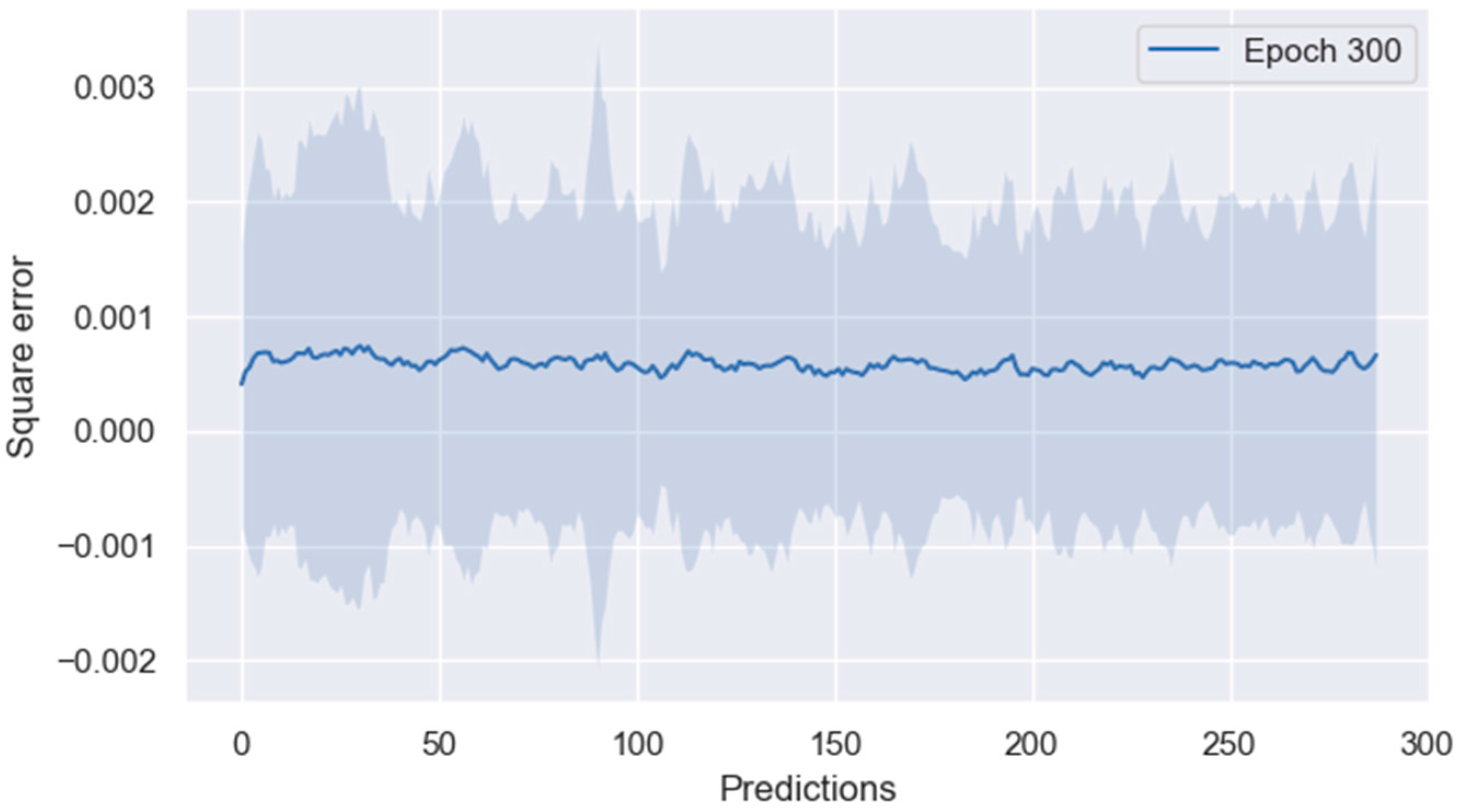
The predictive performance is evaluated as shown in Figure 7.

The predictive model demonstrates robust performance, as evidenced by a Mean Absolute Error (MAE) close to 0.01, specifically 0.010924723. This low MAE indicates that, on average, the absolute difference between the predicted values and the actual values is minimal. Furthermore, the Mean Squared Error (MSE) remains consistently low across all time periods, averaging less than 0.001. This low MSE signifies that the model effectively minimizes large prediction errors, maintaining a high level of accuracy over time. Importantly, there is no observable degradation in predictive performance as the prediction time horizon extends. This stability in error metrics across increasing time periods highlights the model’s capability for long-sequence prediction, underscoring its superiority in maintaining accuracy over extended predictions.

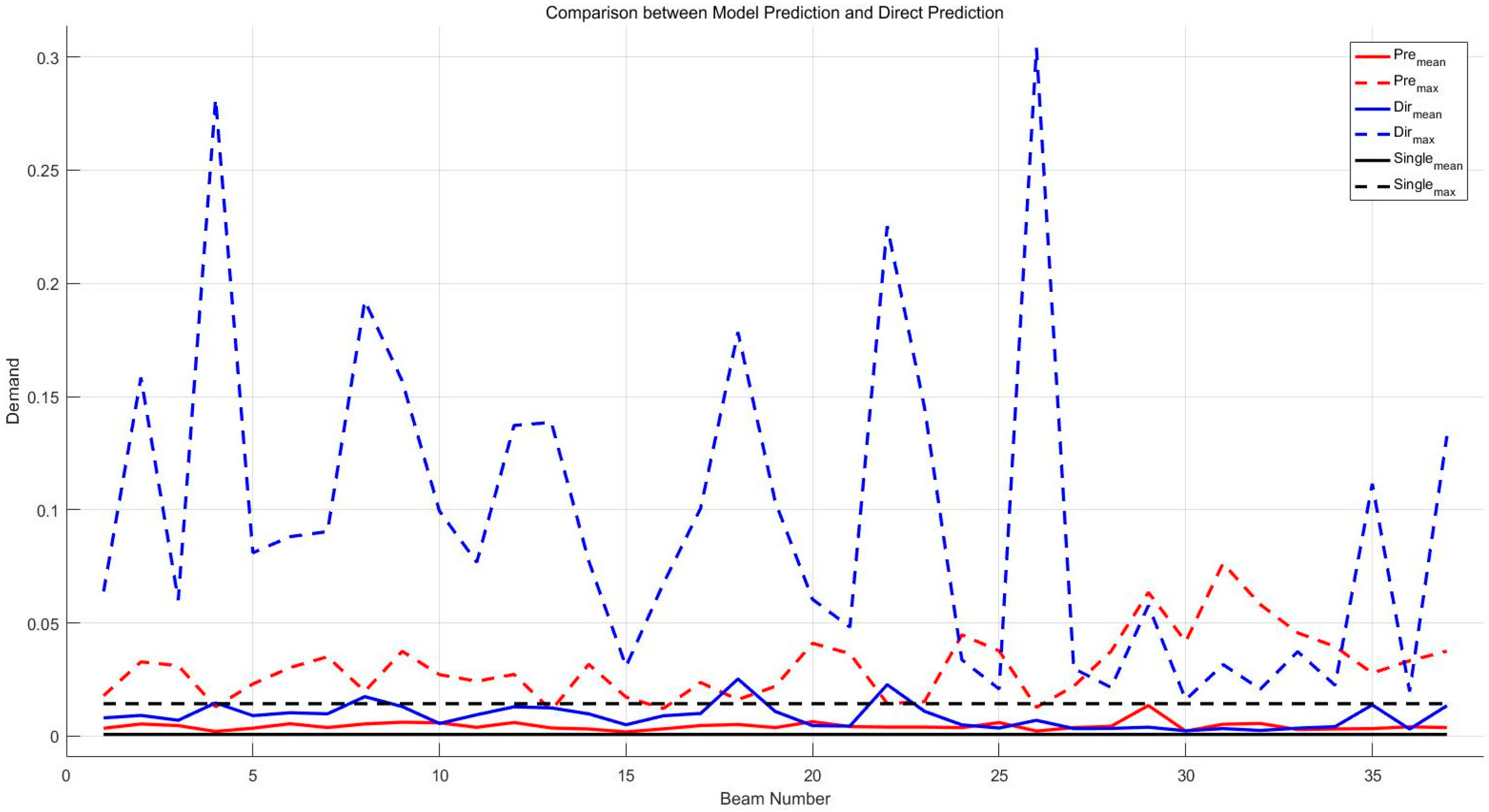
For the demand prediction of communication satellites, which exhibits clear periodicity, the effectiveness of the prediction is compared, as shown in Figure 8. The method of averaging the demand data over 14 days at each time point in a day is used as a reference. The average and maximum MSE obtained from the proposed method are compared with those from direct prediction. The average MSE is calculated by randomly predicting 5000 times for 288 points of data in a day after the model training is completed, while the maximum value is the largest MSE obtained throughout the process.

Using the average value for prediction leads to significant average errors, primarily because it oversimplifies the historical demand data of a single beam and fails to capture its intricate fluctuations and complex patterns. This approach assumes a uniform distribution of demand over time, overlooking the significant variability and nonlinearity inherent in real-world data. As a result, important details such as sudden spikes or drops in demand are smoothed out, leading to a substantial Mean Squared Error (MSE) of up to 0.03 and prediction fluctuations exceeding 0.3, indicating a high degree of instability. Furthermore, the average method neglects temporal dependencies, such as cyclical trends and autocorrelation, which are crucial for accurate forecasting. This lack of insight into the underlying causes of demand variability limits its practical utility for applications requiring reliable and stable predictions. Therefore, while averaging provides a quick and straightforward approach, it is insufficient for capturing the complexity of demand patterns, leading to less accurate and less reliable forecasts.

In contrast, when historical demand data for different beams are input separately into the model, the model is able to learn and adapt to the unique characteristics of each beam. This targeted approach allows the model to identify and capture underlying trends, periodicities, and nonlinear relationships that are not evident when using a simple average. Consequently, the model’s predictive MSE is slightly lower than that obtained through averaging, demonstrating that the model can make more accurate predictions by effectively utilizing the historical data. The model’s ability to maintain a significantly lower maximum MSE fluctuation compared to direct averaging underscores its robustness and stability. This reduction in error volatility is critical for practical use cases, as it implies that the model can provide more consistent and reliable forecasts.

Moreover, the model’s performance highlights its superiority in capturing complex data patterns that are missed by simple averaging. By leveraging historical demand data and focusing on individual beams, the model can account for the nonlinearity and seasonal variations inherent in the data. This ability to predict with higher precision and lower error margins makes it particularly suitable for scenarios that require advanced traffic allocation. The reduced volatility and enhanced stability of the model’s predictions better meet the practical requirements for traffic management, ensuring that resources can be allocated efficiently and effectively.

In summary, while using the average value for prediction offers a quick and straightforward approach, it falls short in terms of accuracy and reliability. The model’s capability to capture and adapt to the specific patterns of each beam provides a more nuanced and stable prediction, making it a superior choice for applications that demand precise and dependable traffic forecasts.

The best results are obtained when historical demand data for beams with similar trends are inputted into a single model for training, yielding an average predictive MSE of 0.0007 and a maximum MSE fluctuation of 0.014, both significantly lower than those of directly using the average value for prediction while maintaining excellent stability.

Integrating historical demand data from beams with similar trends into a single model for training often yields superior results compared to training separate models for each beam individually. This is due to several reasons. Firstly, combining data increases the overall dataset size, providing a richer and more diverse set of samples, which helps the model generalize better and reduces the risk of overfitting to the specific patterns of a single beam. Secondly, beams with similar trends share common patterns, such as periodic fluctuations and nonlinear relationships, which the model can learn more effectively when trained on combined data. By leveraging these shared characteristics, the model enhances its ability to recognize and predict these patterns more accurately.

Additionally, this approach improves the stability and reliability of predictions. Integrating similar beams helps smooth out individual anomalies and noise, leading to more consistent and stable predictions. It also addresses the long-tail distribution problem by balancing the dataset and ensuring that the model is adequately trained across various demand scenarios. Furthermore, training on a combined dataset enhances the model’s robustness, making it more resilient to fluctuations and irregularities that might occur in practical applications. This combined training enables the model to better capture the temporal dependencies and cyclical trends that are crucial for accurate long-term forecasting.

Currently, similarity is determined based on manual inspection and visually inspecting computer-generated charts of the historical demand patterns, where beams showing analogous fluctuations and trends over time are considered similar. Beams with similar trends are often in the same time zone range, which further supports their integration for more accurate modeling. However, the need for a more systematic and reproducible approach is acknowledged. As a future research direction, K-means clustering is planned to be employed to automatically group beams based on their historical demand data. K-means is particularly suitable for this task as it can handle large datasets and identify clusters of similar patterns based on features such as mean demand, variance, and periodicity. This method will enable more effective grouping of beams and provide a detailed, data-driven approach to enhancing model performance. This approach is expected to significantly improve the robustness and accuracy of predictions, ensuring that beams with similar trends are effectively identified and grouped.

It is worth mentioning that the model is well suited for scenarios with strong periodicity, where traffic patterns exhibit regular and predictable cycles. In such environments, the model effectively captures the underlying trends and provides reliable predictions. However, in contexts where traffic patterns are highly variable and exhibit significant randomness, the model’s performance may deteriorate.

5. Conclusions

This paper proposes a method for dynamically predicting traffic demands to improve the efficiency of satellite resource management. Based on real data, the method utilizes a deep learning artificial intelligence algorithm that combines Seq2Seq and LSTM networks. This approach enhances prediction accuracy and has broad applicability, fully considering the demands of mobile terminals such as aviation and maritime ones without the need for extensive statistical parameterization. The method can be extended to various real systems and excels in predicting long time series, enabling stable forecasts of traffic demands over extended periods.

Future work should focus on retraining and fine-tuning the model using data from diverse regions and varying traffic patterns to enhance its adaptability and robustness. This includes employing K-means clustering to group beams based on historical demand data that will improve model performance by identifying clusters of similar patterns.