Audio Steganalysis Estimation with the Goertzel Algorithm

Abstract

Audio steganalysis has been little explored due to its complexity and randomness, which complicate the analysis. Audio files generate marks in the frequency domain; these marks are known as fingerprints and make the files unique. This allows us to differentiate between audio vectors. In this work, the use of the Goertzel algorithm as a steganalyzer in the frequency domain is combined with the proposed sliding window adaptation to allow the analyzed audio vectors to be compared, enabling the differences between the vectors to be identified. We then apply linear prediction to the vectors to detect any modifications in the acoustic signatures. The implemented Goertzel algorithm is computationally less complex than other proposed stegoanalyzers based on convolutional neural networks or other types of classifiers of lower complexity, such as support vector machines (SVD). These methods previously required an extensive audio database to train the network, and thus detect possible stegoaudio through the matches they find. Unlike the proposed Goertzel algorithm, which works individually with the audio vector in question, it locates the difference in tone and generates an alert for the possible stegoaudio. In this work, we apply the classic Goertzel algorithm to detect frequencies that have possibly been modified by insertions or alterations of the audio vectors. The final vectors are plotted to visualize the alteration zones. The obtained results are evaluated qualitatively and quantitatively. To perform a double check of the fingerprint of the audio vectors, we obtain a linear prediction error to establish the percentage of statistical dependence between the processed audio signals. To validate the proposed method, we evaluate the audio quality metrics (AQMs) of the obtained result. Finally, we implement the stegoanalyzer oriented to AQMs to corroborate the obtained results. From the results obtained for the performance of the proposed stegoanalyzer, we demonstrate that we have a success rate of 100%.

1. Introduction

Information security has greatly increased in recent years due to the increased demand for the use of computers and mobile devices. Some fields, such as multimedia encryption systems, steganography, steganalysis, and watermarking [1], have stood out in this field for their attention to information confidentiality. Steganalysis is the science of analyzing and verifying the presence of foreign data in digital files, including audio, images, and videos, through different spatial or frequency techniques. Unlike steganography, which inserts data into digital files, steganalysis detects any changes resulting from the insertion process. When data are inserted into an audio file, the frequency spectrum of the file is modified, which we call this new file stegoaudio. The change in the frequency of the audio file is known as the fingerprint of the audio file [2]. Audio file fingerprints are outliers present in audio files [3].

Therefore, the steganalysis process detects the variation in frequency, or footprint, of the stegoaudio. Footprints can be detected through filtering techniques, frequency analysis, supervised or unsupervised statistical classifications, or statistical analysis [2]. In recent years, various methods have been implemented for stegoimage analysis; however, audio has experienced a slower profession due to the complexity of data processing [4]. Recently, voice communication has become popular among social networks such as WhatsApp, Facebook, TikTok, and YouTube [5]. Communication via voice transmission through smartphones has increased as social networks grow in popularity. These communications require tools that provide greater security and tranquility to end users. Free practical tools exist for hiding secret messages in audio files, such as S-Tools and Hide4PGP for audio files in .wav format or MP3Stego for .mp3 files [5]. In many applications, such as dual-tone multifrequency (DTMF) signals, a digital multifrequency (MF) receiver is necessary to recognize frequency components simply and efficiently [6]. A second-order realization of the Goertzel filter is also favored over the direct DFT because it results in reduced computational burden [6]. The Goertzel algorithm is used to compute the DFT spectra. It can be performed from the perspective of the DFT taken over short time sections of the signal (the time window is fixed) or from the perspective of a filtering operation at a given frequency (the frequency is fixed) [7]. Therefore, the Goertzel algorithm is a faster method of pitch detection than a fast Fourier transform and a DFT for a single frequency) [7].

Linear prediction analysis is a tool that has been used in many fields. It has been used in audio signal processing and is one of the most popular and effective methods, especially in the evaluation of basic speech characteristics, spectrum, low-speed transmissions, speech storage, etc. It can accurately evaluate the characteristics of the audio signal and can correctly represent the time domain and frequency domain characteristics of the audio signal with fewer parameters [5].

In this work, we apply the classic Goertzel algorithm to detect possible frequencies that have been altered by the insertion or alteration of the audio vector in conjunction with linear prediction for the detection of possible altered tones. The final vectors are plotted to visualize the alteration zones. The obtained results are measured qualitatively and quantitatively.

This work focuses on the following main contributions:

• By detecting the differences in frequency of the audio signals, the fingerprints of the files are located to compare the audio files.
• The method proposed here can detect files of the same type as well as text or image files.
• Minimum implementation complexity, unlike methods based on neural networks. The potential frequency range of the alteration of the original audio is identified.

From the analysis of the signal using Goertzel, we can obtain the range of frequencies in which the frequency tones that can represent information other than the original vector are found. Therefore, as shown in the results, it presents an accuracy percentage greater than 93% for detecting stegoaudios.

In the following sections, we explain in detail each of the stages that make up the proposed approach. In Section 2, the methods implemented in this research are described. In Section 3, the results obtained from the frequency analysis implementing the Goertzel algorithm and the corresponding statistical analysis are presented. In the same way, the performance of the proposed method is compared with the performances of methods available in past literature. In the Section 4 shows the results of the statistical coefficients of the comparative analysis of the audio vectors. Finally, Section 5 and Section 6, the final conclusions and discussion of the work are presented.

2. Materials and Methods

Few steganalysis methods exist for audio files; as a consequence, audio steganalysis is a necessary tool for detecting possible intrusions [8]. The popularity of streaming audio files in either .WAV or .MP3 format in digital media can result in vulnerabilities [4]. This requires generating techniques and mechanisms applicable to intervention analysis.

Some works related to the topic of audio file analysis are described in this section. Recent developments have been made in analyzing audio for hidden message detection. These developments include the following documented works.

In 2003, Ozer et al. proposed a universal audio steganalysis technique based on the quality metrics of an audio file. This technique is efficient for both the watermarking and steganographic methods. The idea in [8] is based on statistical evidence that the distortion measures calculated between the original audio file and the file with embedded data should have statistically distinguishable distributions for the information-bearing signals and the stegosignals [8]. Based on these quality metrics, the test files are examined to determine whether the audio is a stegoaudio.

In 2004, Böhme et al. proposed a method based on a block decoder of an MP3 audio file, and subsequently applied a method based on the psychoacoustic model to identify characteristics [9].

In 2005, Johnson et al. proposed a speech record stegoanalysis algorithm based on LSB embedding in conjunction with the Hide4PGP algorithm for files with sampling rates of 44 and 100 to 16 bits per sample [10].

In more recent years (2015), Kuriakose et al. [11] proposed a stegoanalyzer incorporating interframe Markov analysis for audio files modified through MP3Stego.

In 2018, Han et al. applied linear prediction in conjunction with a Support Vector Machine (SVD) with a Gaussian radial basis function (RBF) kernel. This was used as a classifier and coupled with a k-fold cross-validation method to identify the best parameters and thus improve the anomalous feature detection accuracy [5].

In 2020, Chaharlang et al. proposed a steganalysis method based on quantum analysis. His method consists of two sections [1]. The first section is the steganography of the audio file based on the classic Last Bit Significant steganography algorithm but in terms of quantum computing, consisting of steganography in the insertion of data into the least significant fractional qubit (LSFQ) within the amplitude of the audio signal samples. In the second section, steganalysis is performed in a feature extraction module from the audio signal frames and quantum circuits, implementing the KNearest Neighbor (KNN) algorithm and the Hamming distance criterion [1].

In 2022, Ren et al. proposed using the spectrogram as an input feature to extract information. DeepResNet is then applied to learn the representations of distinctive features, and the multiscale spectrograms enrich the diversity of input features [12].

A common analysis tool for frequency analysis in detecting signal frequency changes is the Fast Fourier Transform (FFT); however, its high computational cost complicates its application in architectures with limited processing capacity.

Hence, in this research proposal, we present a stegoanalysis technique for audio files based on an adaptation of the frequency analysis. The analysis is performed in conjunction with a statistical analysis and Audio Quality Metrics (AQM) [8] between the audio signals and possible stegoaudio.

2.1. Stegoanalyzer Process

In this section, each step of the proposed method for the steganalysis of audio files is detailed. To better demonstrate how a steganalyzer works, we begin with a basic description of how steganographic algorithms work.

Steganography is the process of hiding data within a digital medium known as the host medium; in this case, the medium is an audio file [13]. In this work, we implemented the Steghide algorithm. Steghide is designed as a steganographic tool with very good robustness [14]. In general, it consists of the following algorithm [14]: “The embedding algorithm roughly works as follows: At first, the secret data is compressed and encrypted. Then, a sequence of positions of pixels in the cover file is created based on a pseudo-random number generator initialized with the passphrase (the secret data will be embedded in the pixels at these positions). Of these positions, those that do not need to be changed (because they already contain the correct value by chance) are sorted. Then, a graph-theoretic matching algorithm finds pairs of positions such that exchanging their values has the effect of embedding the corresponding part of the secret data”.

Steganalysis consists of the detection of hidden information embedded with the use of steganography tools or techniques in media files [13]. Figure 1 depicts the block diagram of the general basic mechanism for data insertion (steganography). For this investigation, a wav audio file is considered. Our first main input function is x[n], which represents the original audio file, also known as the host file. The other main input function y[x], to the matchpoint is the hide signal on the host function. The matchpoint is the insertion point of the vector to be hidden in the audio vector (host file), which is known as the hiding process. Currently, there are various steganography methods: the classic methods are in the time domain, such as the one known in the insertion of the least significant bit (LSB) [15,16]. There are other methods in the frequency domain, for which it is common to find methods related to the Discrete Wavelet Transform (DWT) and the Discrete Fourier Transform (DFT), to mention a few, and finally, there are methods that present a combination of these domains (time-frequency).

At the end of the process, we obtain a modified audio file, known as stegoaudio, and represent it by the function s’[n]. s’[n] is used to determine if any information is embedded inside the file.

Proposed Stegoanalyzer

In this section, we describe the proposed audio stegoanalyzer. Figure 2 shows a block diagram of the proposed stegoanalyzer. In general, Figure 2 is divided into the 3 main steps of processing the signal to be analyzed: In step 1, the original audio files x[n] and the possible stegoaudio s’[n] are entered. Next, in step 2, the Goertzel algorithm is applied to perform the frequency analysis of the audio vectors $x\left[d\right]$ and $s\prime$. A frequency scan is then executed to detect the characteristic fingerprints of each signal. In step 3, the results obtained from step 1 and step 2 are validated twice. In addition, the statistical dependency between the fingerprints obtained in the first step is analyzed.

Figure 2 depicts the detailed stegoanalyzer process.

• Step 1. Goertzel algorithm

From the Figure 2, the Goertzel algorithm is typically used for detecting the tones produced on a telephone keypad, known as dual-tone multifrequency (DTMF) [6,17,18]. The tones are recognized using the total run of the harmonic current. Therefore, the algorithm can provide a non-zero value when it detects such a harmonic in the frequency range of the input signal. The tested signal is divided by the number of intervals for the analysis. The exact Fast Fourier Transform (FFT) in the range of the reference frequency can then be calculated [19,20]. The procedure for the Goertzel algorithm is detailed below.

In this step, the entire audio vector is scanned to detect the variation in pitch, which can represent the data inserted in the original audio vector.

From the set of data entered, given $x^i$, we initially develop the first sequence as shown below:

$$X\left[k\right]=\sum _{d=0}^{N-1}{x}^i\left[d\right]e^{-\frac{j2\pi kd}{N}},k=\mathrm{0,1},\cdots ,N-1$$

(1)

Multiplying the right side of the equation by $e^{-\frac{j2\pi kd}{N}}=1$, and rearranging the terms yields the following equation [17]:

$$X\left[k\right]=\sum _{d=0}^{N-1}{x}^i\left[d\right]e^{-\frac{j2\pi k(d-N)}{N}},k=\mathrm{0,1},\cdots ,N-1$$

(2)

where $x^i\left[d\right]$ represents audio vector analysts and N is the number of sampling intervals of the signal, d is the position of the current element of the audio vector to be analyzed and k represents the kth element of the FFT. The size of the block N is equivalent to the number of points in the FFT. This value controls the frequency resolution for which the Goertzel algorithm is used, which is also known as the sample interval width [19,20].

Step 1. Frequency scanning: In this step, the audio vector is divided to obtain the sample interval from Equations (5) and (6), where N can take values of 10, 100, 1000, or 44,100. In this paper, we choose N = 100, so the interval width would be 441 samples per second. To detect the frequency interval, these must be multiples of the sample rate/N. The value of N does not necessarily have to be a multiple of two, enabling Goertzel algorithm flexibility with respect to the FFT [19,20]. See Figure 2.

$$X_m\left[k\right]=\sum _{d=0}^{N-1}X\left[d+k\right]e^{-\frac{j2\pi md}{N}}$$

(3)

$$X_m\left[k+1\right]=\sum _{d=0}^{N-1}X\left[d+k+1\right]e^{-\frac{j2\pi md}{N}}$$

(4)

Substituting $p=d+1$ into $X_m^{k+1}$ yields:

$$X_m\left[k+1\right]=\sum _{d=0}^{N-1}X\left[p+k\right]e^{-\frac{j2\pi m(p+1)}{N}}$$

(5)

By factorizing the domains of the exponential factor, we obtain:

$$X_m\left[k+1\right]=e^{j2\pi m/N}\sum _{p=0}^{N-1}X\left[p+k\right]e^{-j2\pi mp/N}+X\left[k+N\right]e^{-\frac{2\pi mN}{N}}·e^{\frac{j2\pi m}{N}}-X[k]e^{j2\pi m/N}$$

(6)

Finally, due to the periodicity of the exponential term $(e^{j2\pi m}=1)$, by substituting in $X_m^k$, the previous expression is simplified to apply the sliding window:

$$X_m\left[k+1\right]=e^{j2\pi m/N}\left[X_m\left[k\right]+X\left[k+N\right]-X\left[k\right]\right]$$

(7)

where $X_m\left[k+1\right]$ represents the component in the frequency of the possible stegoaudio analyzed, m represents the vector to be analyzed, k represents the set of samples to be analyzed, d represents the current analyzed sample, and N represents the total length of the vector.

Step 2. In this step, the statistical analysis is performed. The coefficients of the high-order statistical models, such as asymmetry, kurtosis, and variance, of $\overrightarrow{X}$ are obtained from the time/frequency decompositions extracted from the previous step, with n = 1, 2, …, N. These coefficients provide the characteristics of the statistical distribution of the possible stegoaudio and thus obtain a double validation of the tone frequency that has been identified in the previous step.

• Linear Prediction

Linear prediction analysis is an advanced technology and has been used in many fields. As an important tool utilized in the audio signal process, it has been one of the most popular and effective methods, especially for evaluating the basic speech features such as fundamental tone, formant, spectrum, lower-speed transmissions, voice storage, etc. [5,21].

We propose using linear prediction to verify the error between the components of the possible stegoaudio from the following expression [21,22,23]:

$$\overrightarrow{LP}=Q\overrightarrow{w}=\sum _k{w}_k{Q}_k$$

(8)

where $\overrightarrow{LP}$ is the linear condition, $Q$ is the stegoaudio, and $\overrightarrow{w}$ is given by the transposed vector $Q$. The weights $w_k$ of the coefficients are selected to minimize the estimation of the squared error. The coefficients are selected to minimize the function of the squared error.

$${\rm E}\left(\overrightarrow{w}\right)={\left[\overrightarrow{LP}-Q\overrightarrow{w}\right]}^2$$

(9)

The error in this function is minimized by taking the derivative with respect to $\overrightarrow{w}:\frac{d{\rm E}\left(\overrightarrow{w}\right)}{d\overrightarrow{w}}=2Q^T\left[\overrightarrow{V}-Q\overrightarrow{w}\right]$. Setting this function to zero and solving $\overrightarrow{w}$ yields the following expression [21,22,23]:

$$\overrightarrow{w}={\left(Q^{T}Q\right)}^{-1}{Q}^T\overrightarrow{LP}$$

(10)

The logarithmic error in the linear prediction is given by [17]:

$$\overrightarrow{{\rm E}}={log}_2\left(\overrightarrow{V}\right)-{log}_2\left(\left|Q\overrightarrow{w}\right|\right)$$

(11)

• Pseudocode

In summary, the steps of the proposed algorithm are as follows:

• Separation of audio vectors into their respective left and right channels.
• The audio vectors $x^i\left[d\right]$ and ${s\prime }^i\left[n\right]$ are entered according to the Goertzel algorithm. The length of each vector is in accordance with the sampling frequency of 44,100 samples per second, which is the standard for audio files with the *.wav extension.
• From step 1, the audio vector $x^i\left[d\right]$ and ${s\prime }^i\left[n\right]$ samples are subdivided into sets with length N = 100. Corresponding to the sliding window of the Goertzel algorithm:
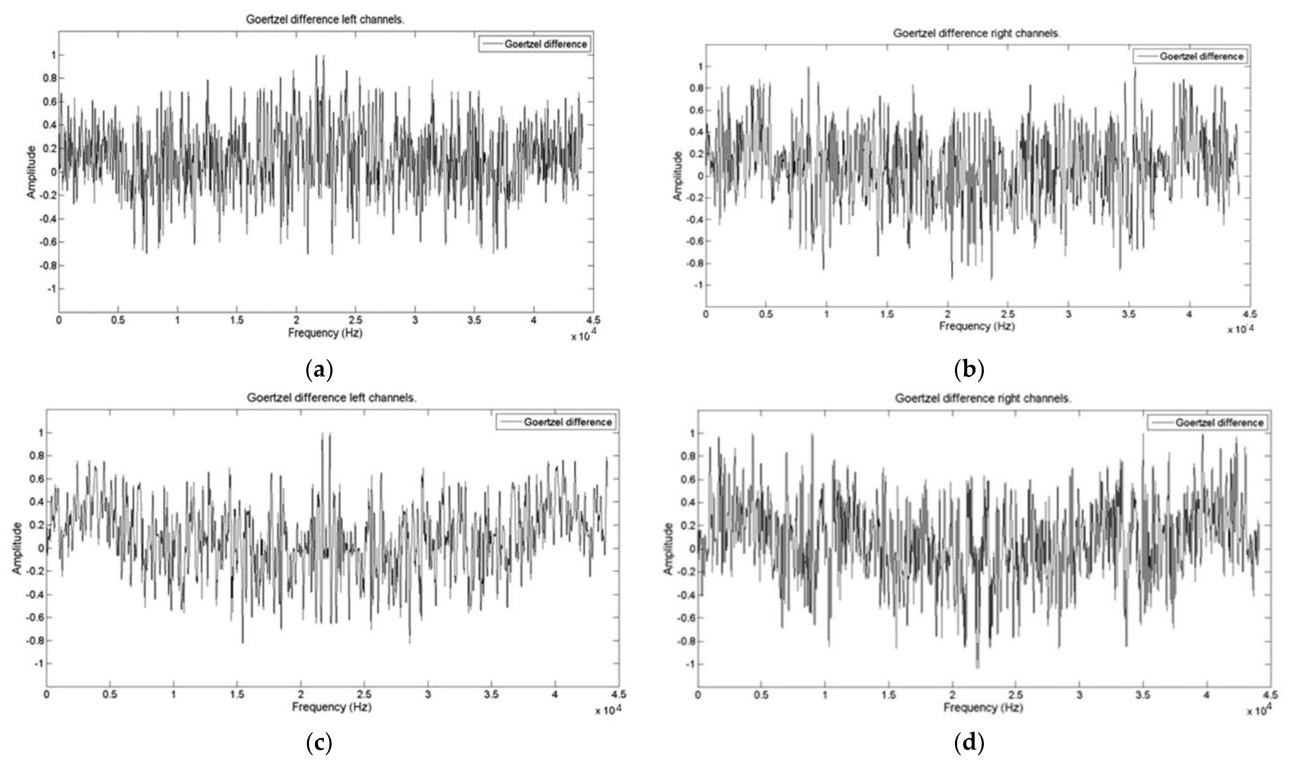
• The vectors obtained from points 1 and 2 are subtracted to obtain the vector resulting from its frequency spectrum.
• In Step 3, the statistical parameters are applied as the mean, variance, covariance, skewness, kurtosis, energy, and AQM of the signals are calculated to evaluate the performance of the proposed stegoanalyzer.
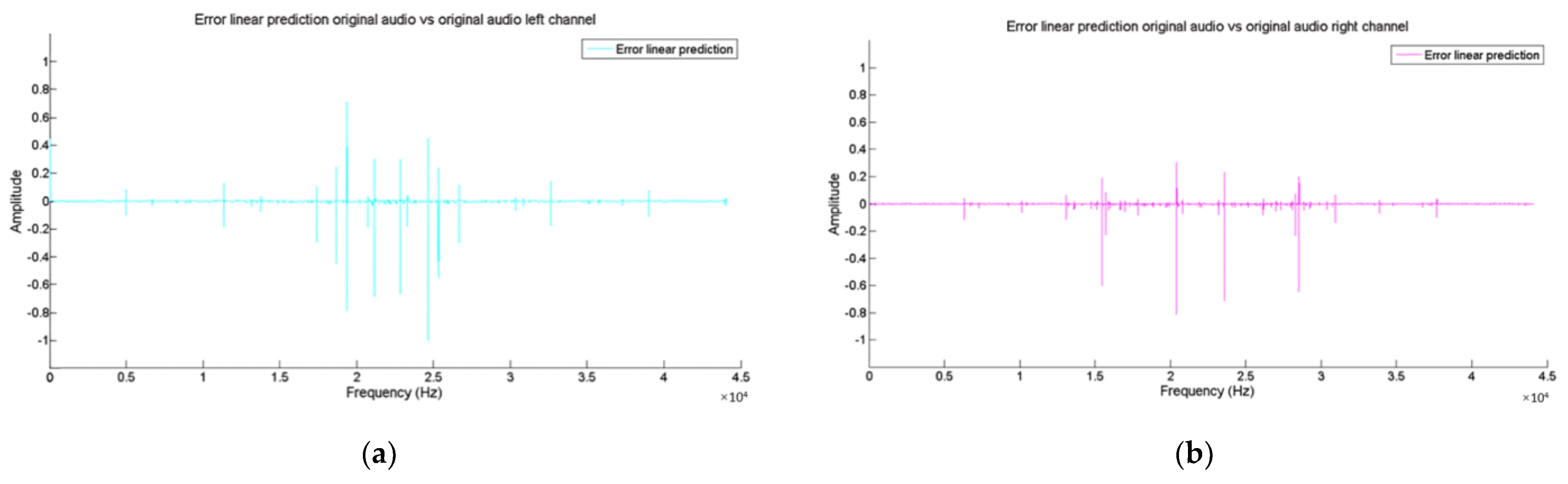
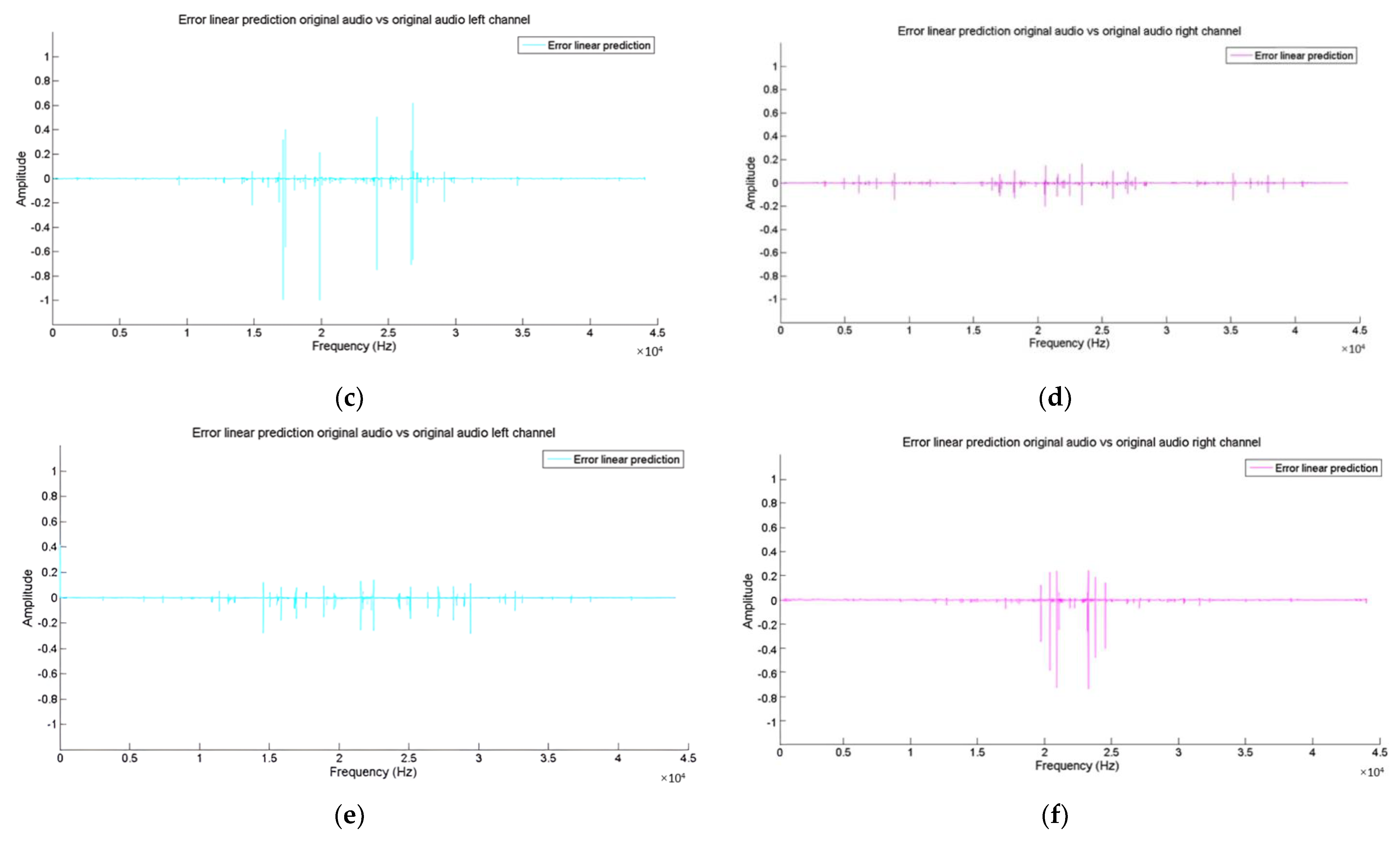
• Finally, as a final step, the error values obtained from step 4 are compared to perform the linear prediction for the vectors $x^i\left[d\right]$ and ${s\prime }^i\left[d\right]$.

3. Performance Evaluation

The tests were conducted on a Windows 10 platform with an AMD RYZEN computer. The audio information vectors used have a .wav format of 16 bits, stereo with a sample rate of 44, 100 Hz. The stegoaudios were generated using the Steghide program [14,24], a steganography program that allows information to be hidden in different types of images and audio.

Two types of tests were carried out: the first audio files with hidden audio, and the second test was carried out with audio files inserting images and text. The hidden files used are audio files in .wav format of 16 bits, mono with a sample rate of 44, 100 Hz. The tests for the proposed algorithm were performed with a group of audio vectors in 10 pairs, each of them comprising an audio vector identified as the original audio and an audio vector labeled as a possible stegoaudio. The tests consisted of analyzing each pair of vectors according to the procedure described in the section. The results obtained during each step of the stegoanalyzer process are detailed below.

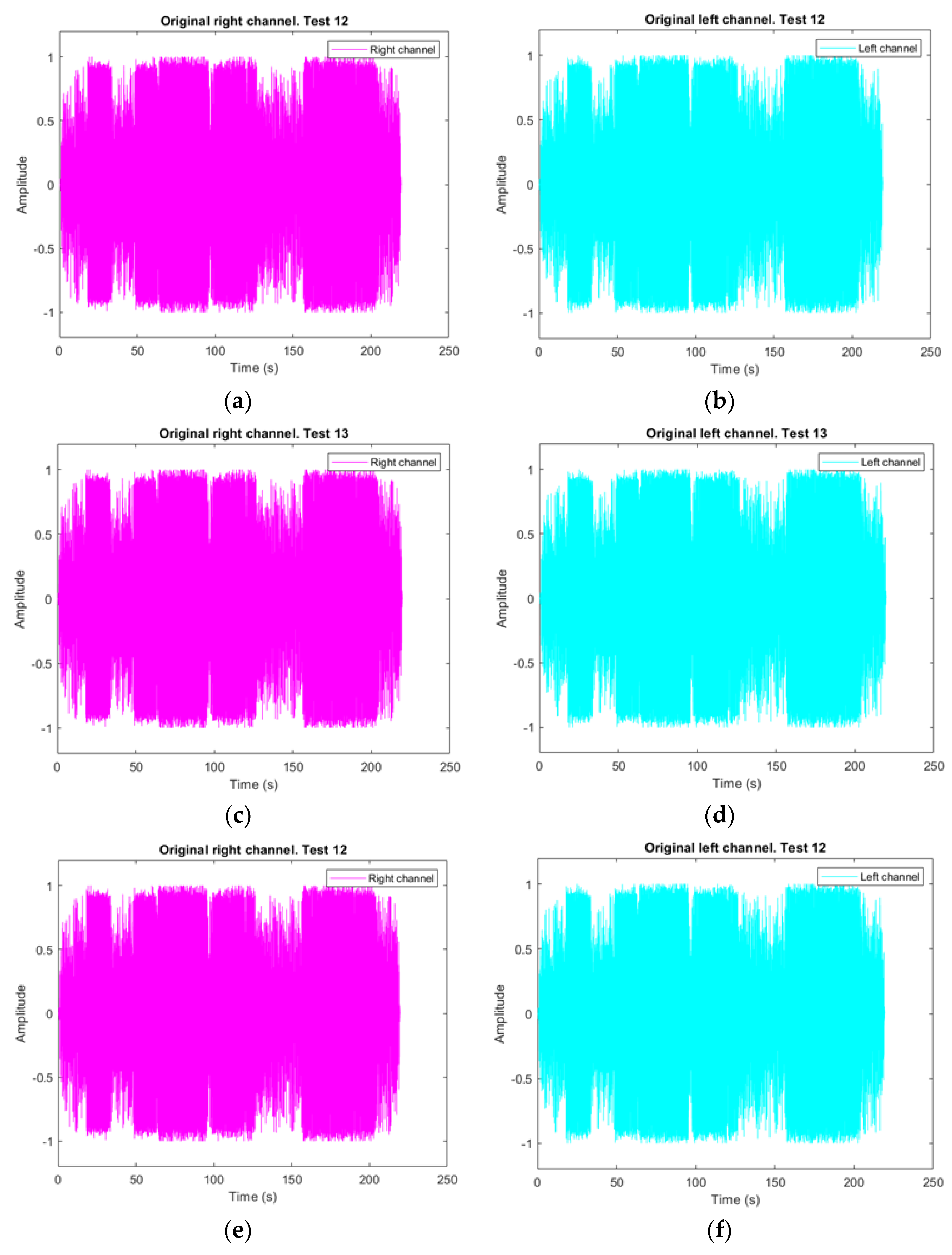
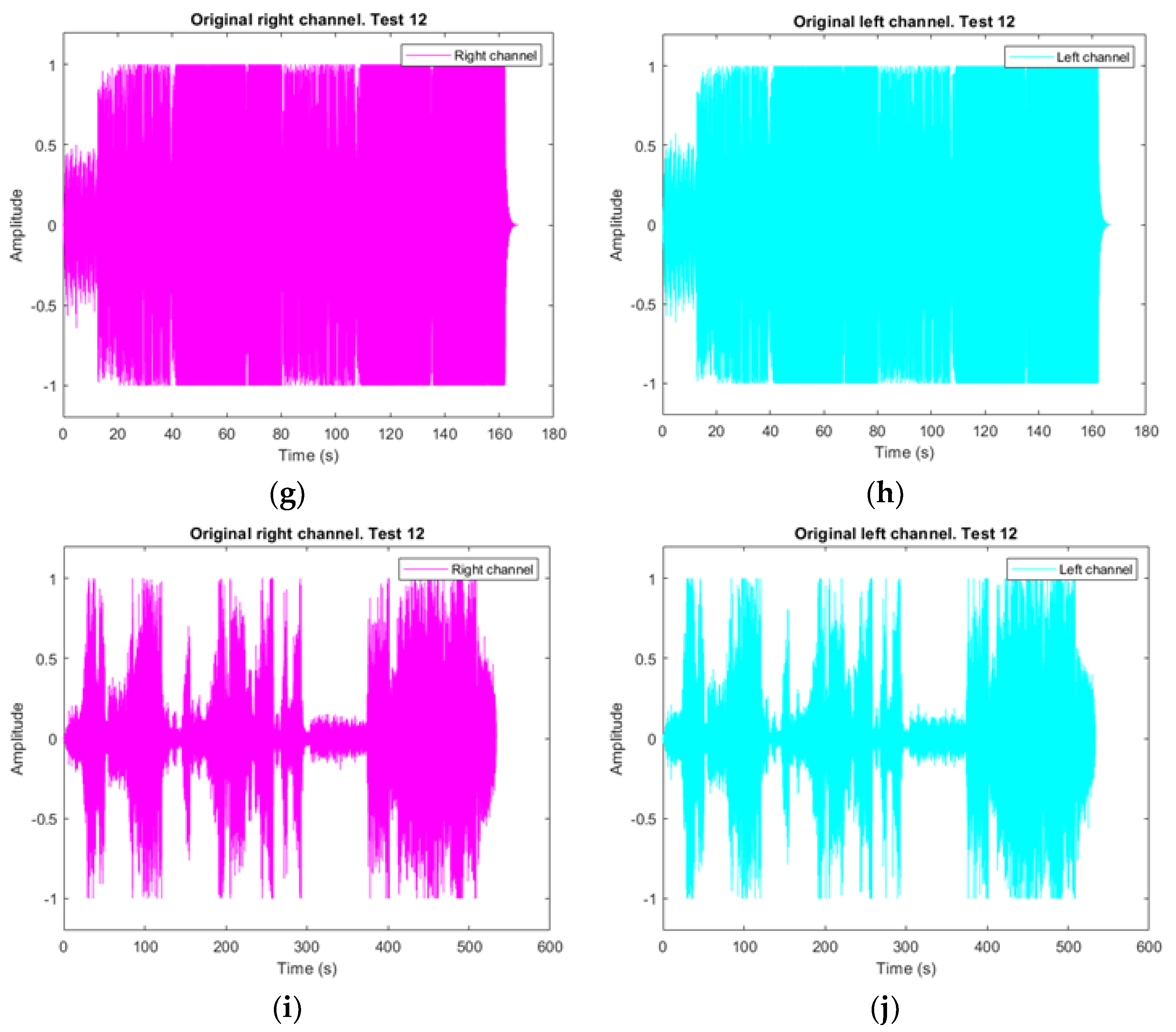
3.1. Vector Audio Decomposition

3.1.1. Original Audio Vector Decomposition

To validate the performance of the proposal made in the detection of possible stegoaudios, the tests were divided into two parts; the first block of audio files was carried out with tests only of possible attacks of audio files with other audio files. The second block of tests was carried out with audio files with possible stegoaudios attacked with text and images. Next, we visualize the results obtained qualitatively:

3.1.2. First Test. Audio Files with Audio File Attacks

The signals obtained from the original audio files are shown in Figure 3. The pair of audio vectors were preprocessed by separating each vector into its respective information channels, left and right. The left and right channels of the audio vectors were treated separately, as shown in Figure 3. Figure 3a,c,e,f show the right vector signals of the original audio signal. Figure 3b,d,f,h show the left vector signals of the original audio signal.

3.1.3. Test 2. Audio Files with Text and Image File Attacks

The signals obtained from the original audio files are shown in Figure 4. The pair of audio vectors were preprocessed by separating each vector into its respective information channels, left and right. The left and right channels of the audio vectors were treated separately, as shown in Figure 4. Figure 4a,c,e,g,i show the right vector signals of the original audio signal. Figure 4b,d,f,h,j show the left vector signals of the original audio signal.

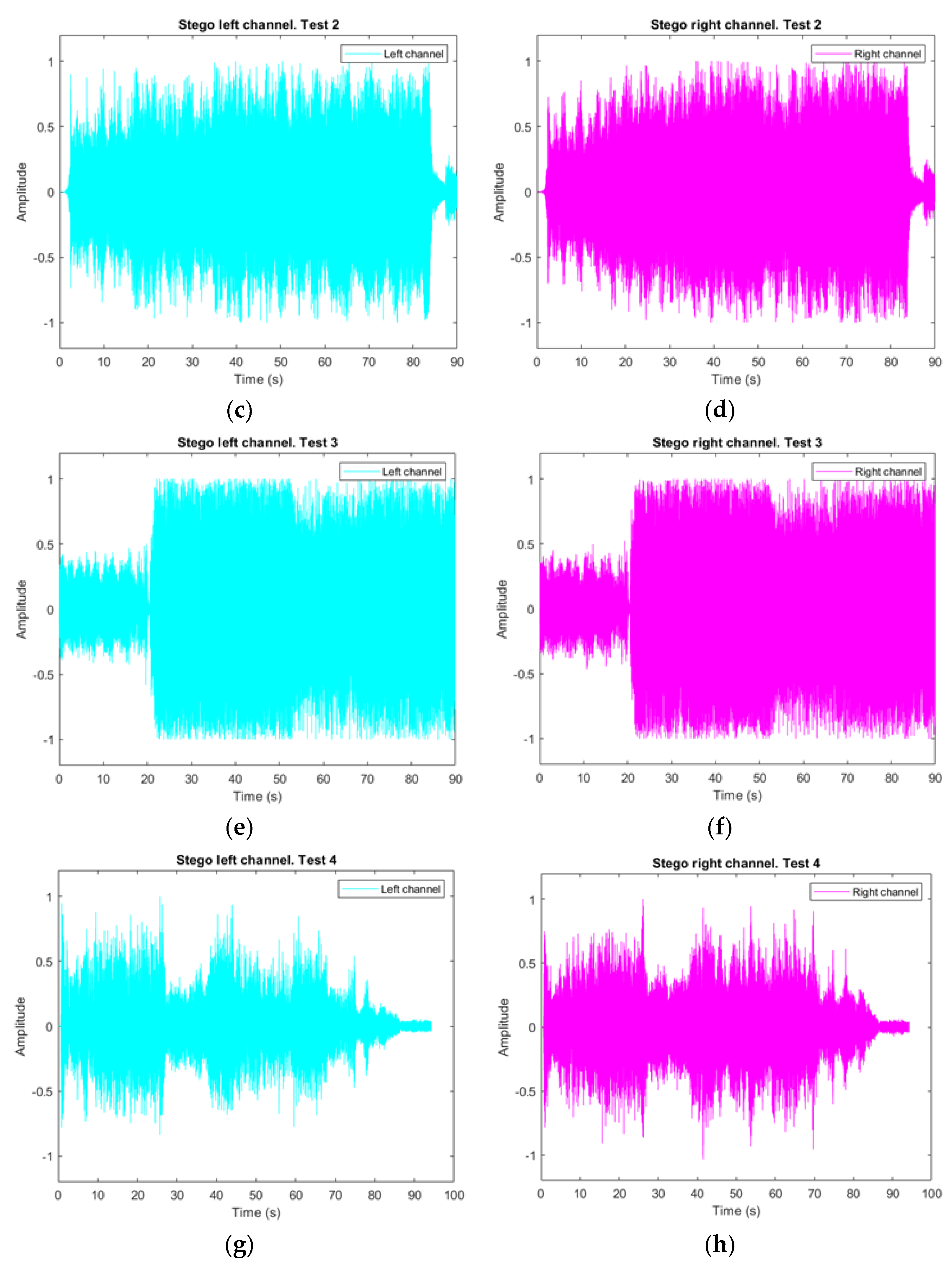
3.2. Stegoaudio Vector Decomposition

Similarly, in Figure 5, we show the vectors of the left and right channels of the stegoaudio.

Test 1. Figures referring to the possible stegoaudios. Audio files with audio files.

3.3. Vector Audio Comparison

Test 2. Figures referring to the possible stegoaudios. Audio files with text and image file attacks.

To qualitatively compare the original and stegoaudio vectors shown in Figure 3 and Figure 4, Figure 5 and Figure 6a–f were obtained. There is no visual variation present between the original audio and the stegoaudio. Therefore, whether there is a perceptible alteration in said vectors cannot be determined. The results of these comparisons are shown in Figure 7 and Figure 8. The graphics illustrate that the channels of both vectors coincide qualitatively with the information contained; thus, hidden information is not detected after analysis. To complete the double analysis, we next conduct an analysis of the frequency spectrum.

Stego audio vector figures:

Figure 6. Graphics of the left and right channels of the stegoaudios. (a) Left channel of the stegoaudio in analysis. (b) Right channel of the stegoaudio in analysis. (c) Left channel of the stegoaudio in analysis. (d) Right channel of the stegoaudio in analysis. (e) Left channel of the stegoaudio in analysis. (f) Right channel of the stegoaudio in analysis. (g) Left channel of the stegoaudio in analysis. (h) Right channel of the stegoaudio in analysis. (i) Left channel of the stegoaudio in analysis. (j) Right channel of the stegoaudio in analysis.

Figure 6. Graphics of the left and right channels of the stegoaudios. (a) Left channel of the stegoaudio in analysis. (b) Right channel of the stegoaudio in analysis. (c) Left channel of the stegoaudio in analysis. (d) Right channel of the stegoaudio in analysis. (e) Left channel of the stegoaudio in analysis. (f) Right channel of the stegoaudio in analysis. (g) Left channel of the stegoaudio in analysis. (h) Right channel of the stegoaudio in analysis. (i) Left channel of the stegoaudio in analysis. (j) Right channel of the stegoaudio in analysis.

Audio vector comparative figures:

Figure 7. Comparative graphics of the original audio channels and the ones of the possible stegoaudios. (a) Comparison between the left channels of the original audio and the possible stegoaudio in analysis. (b) Comparison of the right channels of the original audio and the possible stegoaudio in analysis. (c) Comparison between the right channels of the original audio and the possible stegoaudio in analysis. (d) Comparison between the left channels of the original audio and the possible stegoaudio in analysis. (e) Comparison between the right channels of the original audio and the possible stegoaudio in analysis. (f) Comparison between the left channels of the original audio. (g) Comparison between the left channels of the original audio and the possible stegoaudio in analysis. (h) Comparison of the right channels of the original audio and the possible stegoaudio of analysis the possible stegoaudio in analysis.

Figure 7. Comparative graphics of the original audio channels and the ones of the possible stegoaudios. (a) Comparison between the left channels of the original audio and the possible stegoaudio in analysis. (b) Comparison of the right channels of the original audio and the possible stegoaudio in analysis. (c) Comparison between the right channels of the original audio and the possible stegoaudio in analysis. (d) Comparison between the left channels of the original audio and the possible stegoaudio in analysis. (e) Comparison between the right channels of the original audio and the possible stegoaudio in analysis. (f) Comparison between the left channels of the original audio. (g) Comparison between the left channels of the original audio and the possible stegoaudio in analysis. (h) Comparison of the right channels of the original audio and the possible stegoaudio of analysis the possible stegoaudio in analysis.

Figure 8. Graphics of the spectrum magnitudes of the left and right channels of the original audio. (a) Magnitude spectrum of the left channel of the original audio in analysis. (b) Magnitude spectrum of the right channel of the original audio in analysis. (c) Magnitude spectrum of the left channel of the original audio in analysis. (d) Magnitude spectrum of the right channel of the original audio in analysis. (e) Magnitude spectrum of the left channel of the original audio in analysis. (f) Magnitude spectrum of the right channel of the original audio in analysis.

Figure 8. Graphics of the spectrum magnitudes of the left and right channels of the original audio. (a) Magnitude spectrum of the left channel of the original audio in analysis. (b) Magnitude spectrum of the right channel of the original audio in analysis. (c) Magnitude spectrum of the left channel of the original audio in analysis. (d) Magnitude spectrum of the right channel of the original audio in analysis. (e) Magnitude spectrum of the left channel of the original audio in analysis. (f) Magnitude spectrum of the right channel of the original audio in analysis.

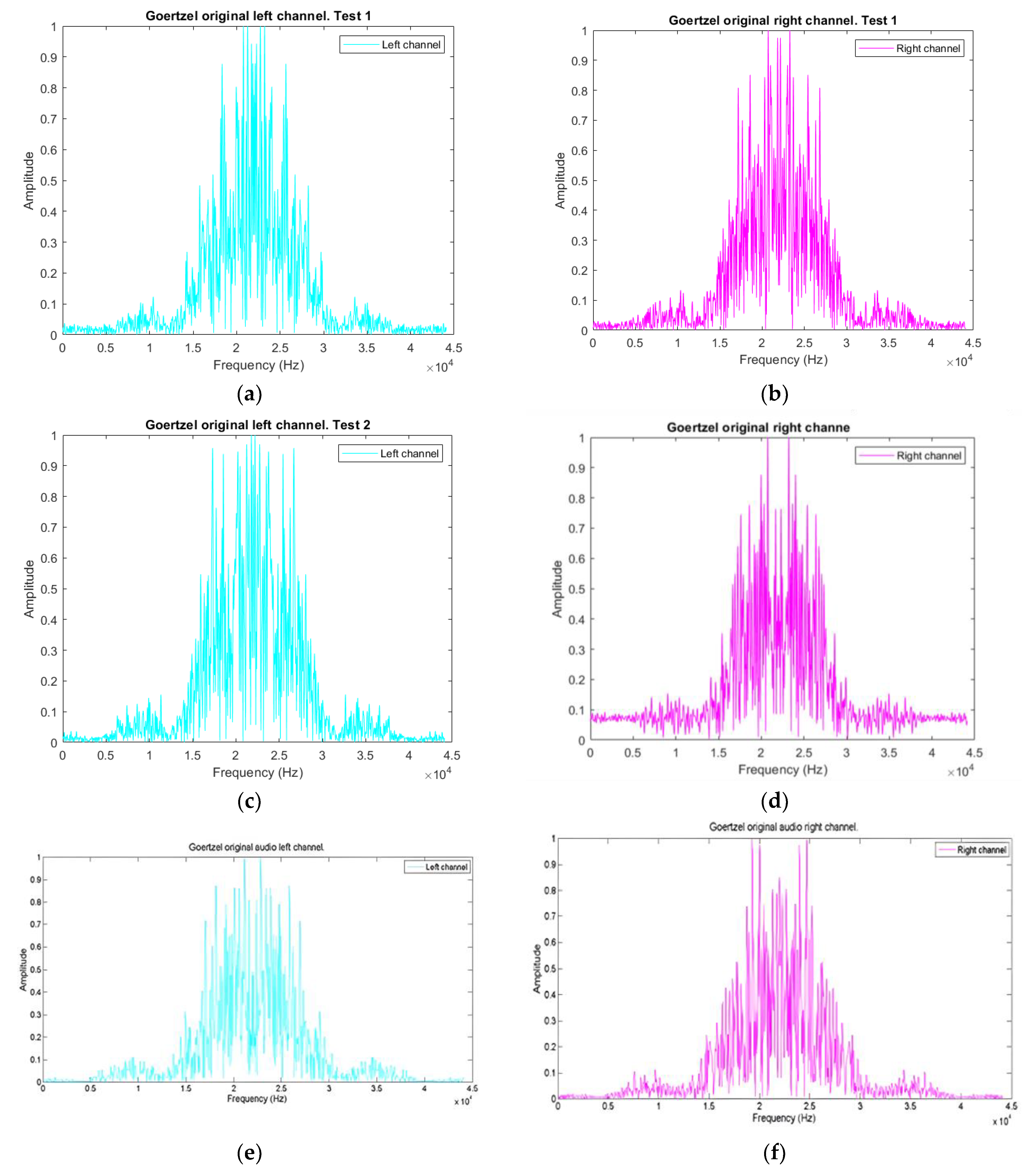
3.4. Frequency Analysis Decomposition

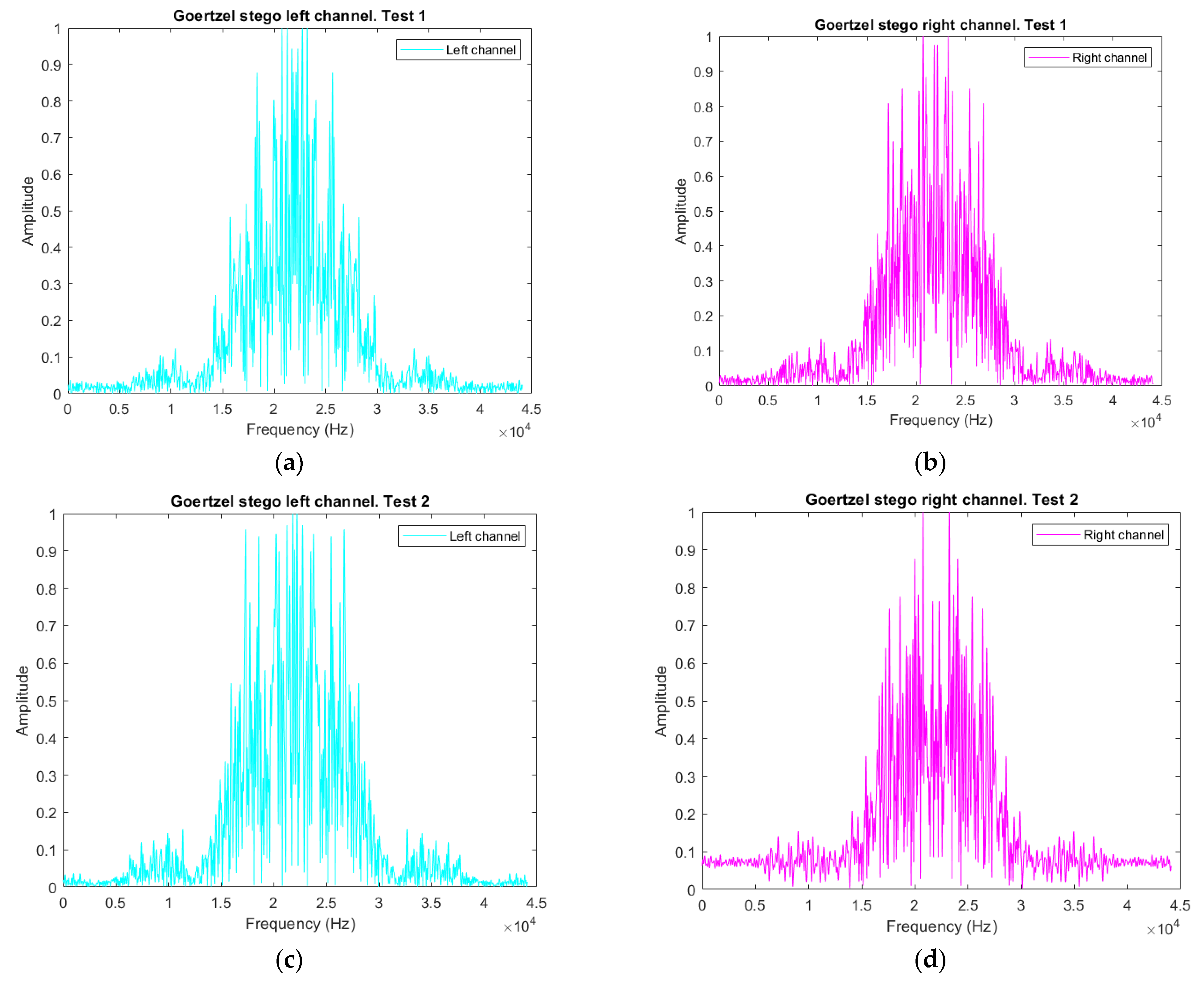
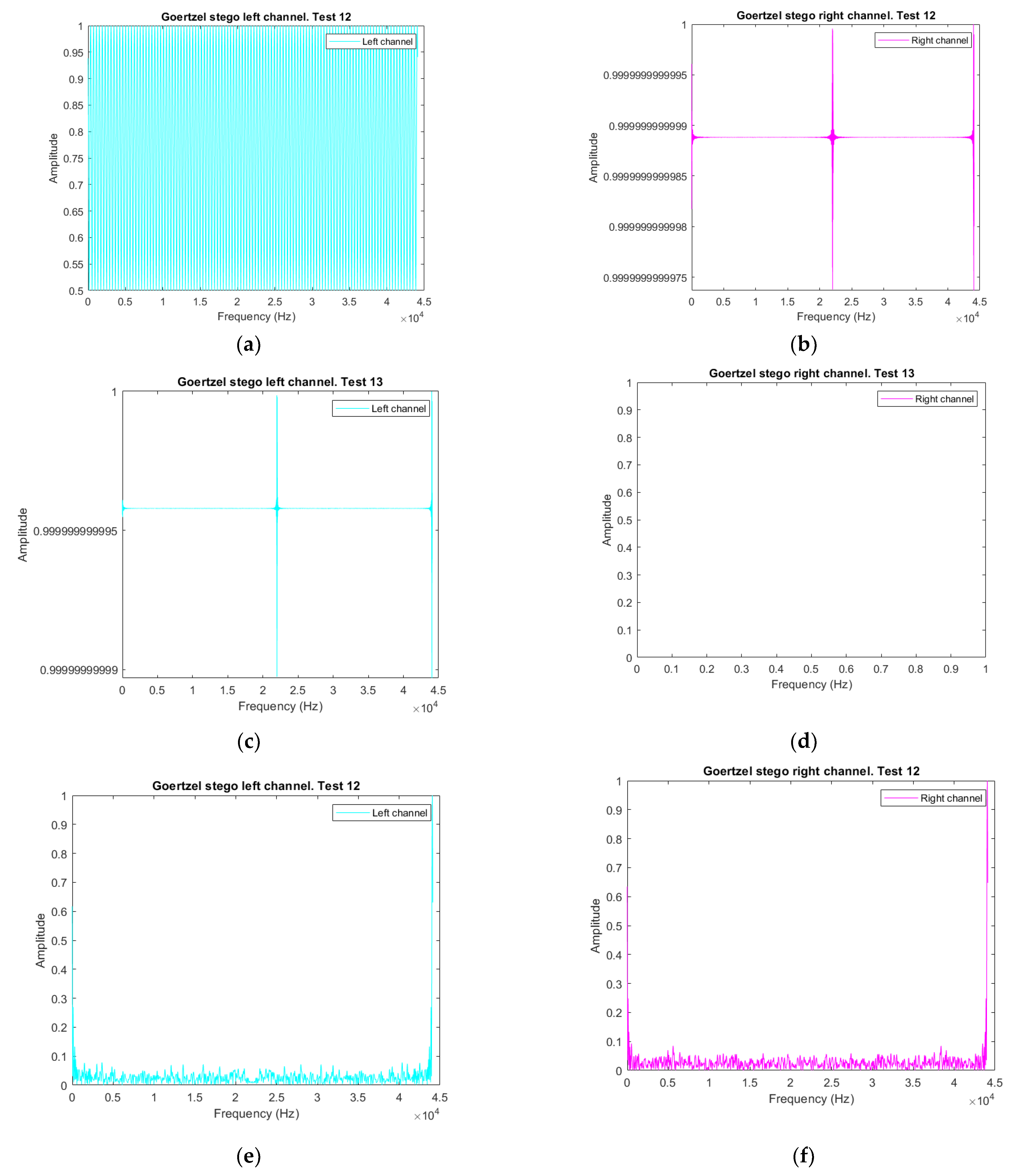
3.4.1. Goertzel Algorithm for Frequency Scanning Audio Vectors

For steps 2, 3, and 4, after separating the audio vector into left and right channels, we performed a frequency spectrum analysis using the Goertzel algorithm. The Goertzel algorithm was applied to each separated channel to obtain their frequency spectrums. The separated vectors preserved a standard sampling rate of 44,100 samples per second in wav audio files, with N = 100.

Test 1. Audio files without attacks

As a result, vectors corresponding to the frequency spectrums of the left and right channels of the original audio vectors were obtained, as shown in Figure 8a–f. Each resulting vector contains the magnitude of the information contained in the frequency components that conform to the audio vectors.

Similarly, the Goertzel algorithm was applied to possible stegoaudios. Figure 9a–f, shows the frequency spectrum of the channels of the possible stegoaudio vector.

Audio comparison original audio analysis Goertzel vs. stegoaudio analysis Goertzel. Subsequently, Figure 10 shows graphically the difference between the analysis of the original audio and the supposed stegoaudio.

From Figure 10a,c,e, we can see in the graphs the range of frequencies in red. These belong to the tones (fingerprints) that have been detected in the right channel of the audio vector as possible information not belonging to the original audio vector. We observe this in a similar way in Figure 10b,d,f; the graphs obtained from the analysis in the left channel are presented in red. From this analysis we conclude that there is information added to the audio vector.

Test 2. Audio files with text and image files.

Goertzel algorithm for frequency scanning audio vectors. As a result, the vectors corresponding to the frequency spectrums of the left and right channels of the original audio vectors were obtained, as shown in Figure 11a–f. Each resulting vector contains the magnitude of the information contained in the frequency components that conform to the audio vectors.

Stegoaudios. Similarly, the Goertzel algorithm was applied to the possible stegoaudios. Figure 12a–f, shows the frequency spectrum of the channels of the possible stegoaudio vector.

From the graphs in Figure 11 related to the original audio vectors, we can see that the Goertzel algorithm did not detect any tone outside the frequency range of the vector (vector without information). Unlike the graphs shown in Figure 12a,c,e corresponding to the left channel of the audio vector, the tone detection included in the frequency range of the possible stegoaudio (image and inserted text) is displayed. Similarly, for Figure 12b,d,f representing the right channel of the possible stegoaudio, the frequency variations of this vector are shown.

Audio comparison: original audio analysis Goertzel vs. stegoaudio analysis Goertzel.

Figure 13 shows the difference between the analysis of the original audio and the supposed stegoaudio.

3.4.2. Audio Vector Comparison

Using the frequency spectrum in each of the information channels, the original audios and corresponding possible stegoaudios were compared. Figure 10a–f shows the comparative graphics, which illustrate that the information contained by the audio vectors differs; this discrepancy is visible only in the frequency domain. The blue line graphic corresponds to the frequency spectrum of the original audio, while the red line graphic corresponds to that of the possible stegoaudio vector. The most notable differences in the red lines are illustrated in the left and right parts of each graph.

Notably, in contrast to the time domain comparison of channels shown in Figure 7, this analysis reveals that information is hidden in the vectors.

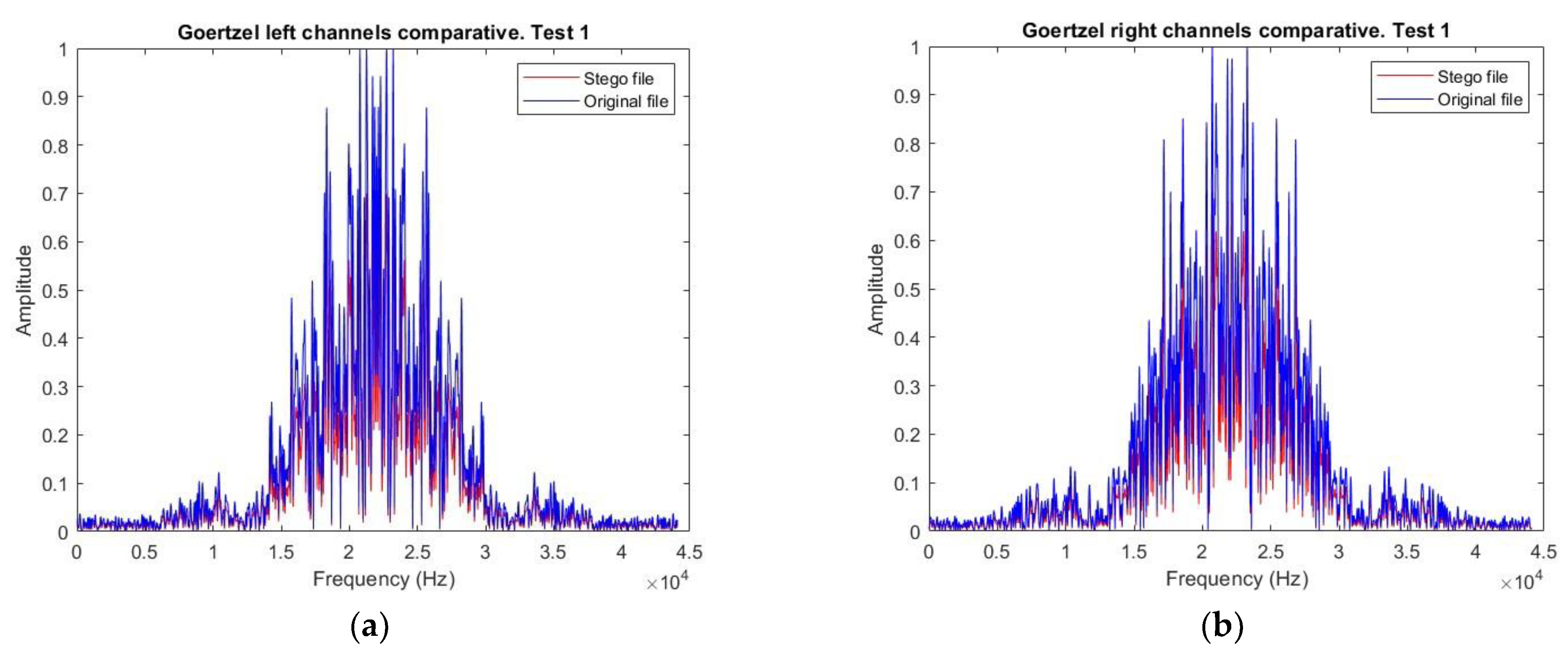
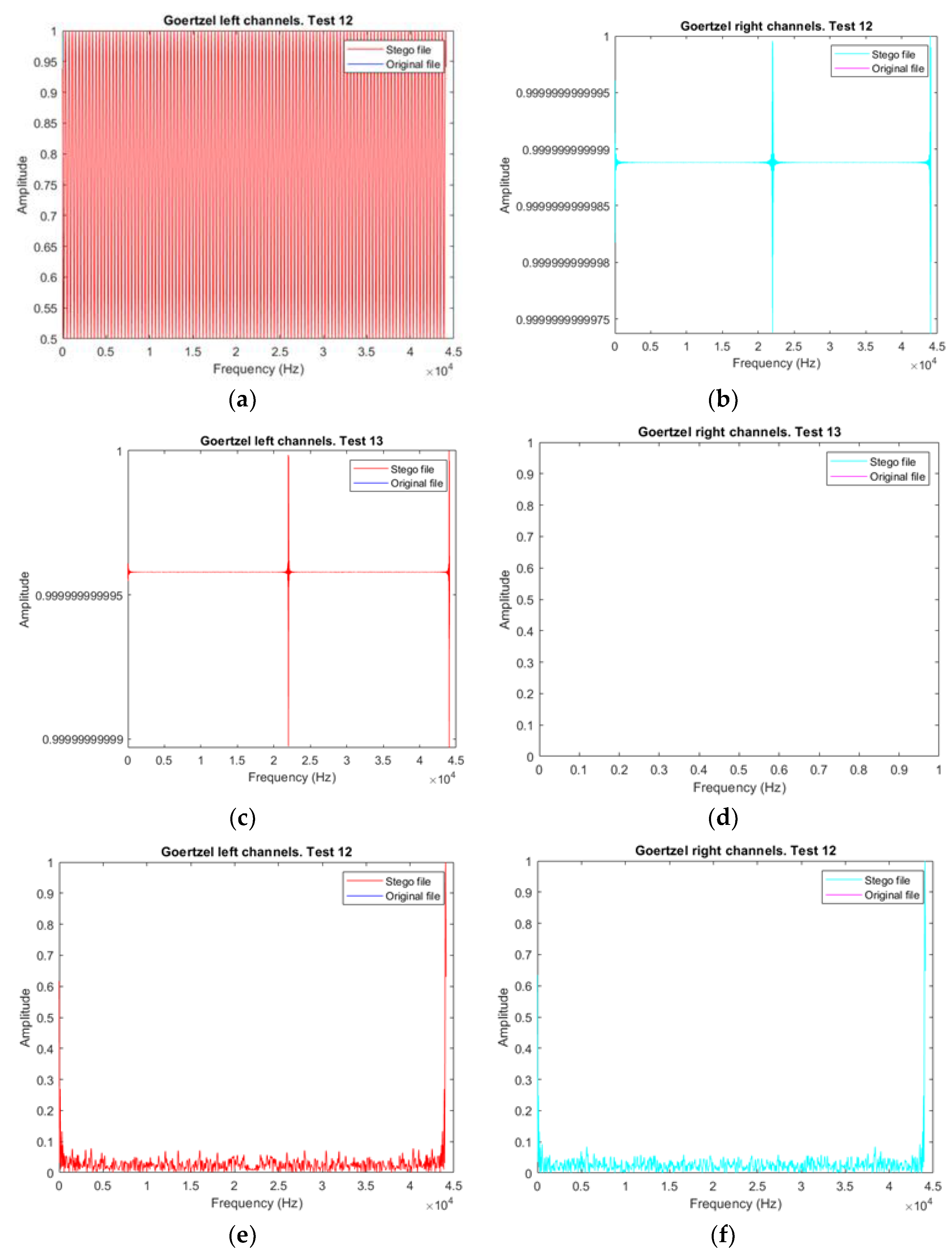
3.4.3. Goertzel Vector Audio Comparison

To verify and validate the presence of unexpected signals, we illustrate the differences between the graphs obtained from the original vector and the vectors with possible additional information. In Figure 14a–e, we show the variations obtained between the audio samples in Figure 14. If no variation exists between the spectrums, an amplitude of 0 is shown in each of the frequency components of the original audio and the stegoaudio. Nonetheless, each of the channels exhibits variations. Some hidden information present in the audio is not perceptible by human hearing, which is common when the concealment procedure of diverse steganography algorithms is applied to audio.

Test 1. The difference graphs are shown with Goertzel analysis between the original file and the supposed stegoaudio (audio files only).

To confirm the results obtained from the Goertzel algorithm shown in Figure 11 and Figure 12, we calculate the difference between the original audio vectors and the possible stegoaudios. Figure 14 shows these differences in both the right channel and the left channel, displaying the detected tones (fingerprints) more precisely.

Test 2. Figure 15 shows the results obtained from the difference in audio signals between the original file and the supposed stegoaudio (text and image files).

In Figure 15, we can see the differences between the original audio vectors and the possible stegoaudios attacked with images. In Figure 15a,c,e, we observe the detected frequency tones. The same is true for Figure 15b,d,f.

In addition to the detection of tones that do not correspond to the original audio vector, we can add a Goertzel computational cost. In [18], it was shown that for real input data of length N, the calculation of the Goertzel algorithm requires 3N operations with a single frequency, so it is more efficient than the FFT if the number of desired frequencies K does not exceed 2log 2N. Have a window of length N = 1024. Therefore, it would mean that the Goertzel algorithm is faster than other types of transforms, such as the FFT [25].

4. Statistical Coefficient Results

To quantitatively evaluate the performance of the proposed steganalyzer, we obtained the higher-order statistical coefficients. We also added classic estimates of noise estimation metrics in various media, such as images or audio files, to these coefficients. The mean squared error (MSE) was the considered metric. The coefficients of the statistical high order considered for the comparison include the mean, the standard deviation, the variance, the asymmetry, and the kurtosis [26,27]. As mentioned in Section 2, these coefficients allow us to identify the distinctive characteristics of the distribution of information and, in this case, of the compared audio vectors.

The first coefficient of the high statistical order (mean) allows us to identify the average magnitude of the information in each analyzed vector. This value allows us to visualize the variation in the signal with respect to its central value.

The standard deviation and variance show the differences between the remaining magnitudes and the obtained mean magnitude. In addition, the signal distortion measurement can be visualized.

The skewness indicates in which direction there is a greater amount of information; the skewness value is positive when it is on the right (high frequencies) and negative on the left (low frequencies). Finally, kurtosis shows the concentration of the vector information in relation to the average, that is, if the information of the vector is more concentrated in the center or at the borders.

Table 1. Coefficients of high statistical order calculated for each of the audio pairs.

Test	Mean		Standard Deviation		Variance		Skewness		Kurtosis		Average Difference Per layer
	Left	Right	Left	Right	Left	Right	Left	Right	Left	Right	Left	Right
1	0.1331	0.1412	0.1920	0.1962	0.0369	0.0385	2.0433	1.8591	6.9245	6.0740	1.8659	1.6618
	0.1383	0.1444	0.1941	0.1942	0.0377	0.0377	2.0488	1.8774	6.9224	6.1448	1.8682	1.6797
2	0.1557	0.1309	0.2170	0.1860	0.0471	0.0346	1.7994	1.9302	5.5369	6.4662	1.5512	1.7495
	0.1565	0.1611	0.2158	0.1643	0.0466	0.0270	1.8125	2.0356	5.5893	6.8439	1.5641	1.8463
3	0.1275	0.1313	0.1862	0.1766	0.0347	0.0312	2.1355	1.9504	7.4058	6.5890	1.9779	1.7757
	0.1335	0.1353	0.1816	0.1732	0.0330	0.0300	2.2027	2.0194	7.7986	6.9441	2.0698	1.8604
4	0.1263	0.1205	0.1854	0.1764	0.0344	0.0311	2.0611	2.1085	6.8736	7.3121	1.8561	1.9497
	0.1272	0.1309	0.1841	0.1766	0.0339	0.0312	2.0738	2.1370	6.9456	7.3841	1.8729	1.9633
5	0.1034	0.1415	0.1555	0.2102	0.0242	0.0442	2.2328	1.9909	8.1453	6.3936	2.1142	1.7560
	0.1055	0.1446	0.1536	0.2098	0.0236	0.0440	2.2692	1.9909	8.3542	6.3640	2.1812	1.7506
6	0.1331	0.1412	0.1920	0.1962	0.0369	0.0385	2.0433	1.8591	6.9245	6.0740	1.8659	1.6618
	0.1361	0.1420	0.1876	0.1944	0.0352	0.0378	2.0567	1.8777	7.0045	6.1407	1.8840	1.6785
7	0.1557	0.1309	0.2170	0.1860	0.0471	0.0346	1.7994	1.9302	5.5369	6.4662	1.5512	1.7495
	0.1555	0.1317	0.2140	0.1852	0.0458	0.0343	1.8278	1.9390	5.6717	6.5146	1.5829	1.7609
8	0.1275	0.1313	0.1862	0.1766	0.0347	0.0312	2.1355	1.9504	7.4058	6.5890	1.9779	1.7757
	0.1332	0.1380	0.1827	0.1764	0.0334	0.0311	2.1572	2.0062	7.4645	6.8348	1.9942	1.8373
9	0.1263	0.1205	0.1854	0.1764	0.0344	0.0311	2.0611	2.1085	6.8736	7.3121	1.8561	1.9497
	0.1272	0.1222	0.1854	0.1772	0.0344	0.0314	2.0689	2.1083	6.9027	7.3051	1.8637	1.9488
10	0.1034	0.1415	0.1555	0.2102	0.0242	0.0442	2.2328	1.9909	8.1453	6.3936	2.1322	1.7560
	0.1076	0.1478	0.1539	0.2105	0.0237	0.0443	2.2941	2.0060	8.4384	6.4523	2.1035	1.7721

shows the obtained mean, skewness, variance, standard deviation, and kurtosis values. These results indicate small variations in the values obtained from the mean, standard deviation, variance, skewness, and kurtosis. For reasons of space, we added tests of only the 10 combinations examined, the stegoaudios modified, and differing values were obtained from the original audios, showing evidence that the frequency components of the audios have been modified.

From Table 1, the numbers highlighted in bold are the values that denote that there is an alteration in the audio vectors. The obtained results reveal that information has been hidden inside the stegoaudios. From the results obtained we observe that the most affected vector is audio test #1. The insertion of this information modifies, in a similar way, all the host vectors based on the results obtained for the mean, standard deviation, variance, skewness and kurtosis. In each of the tests conducted on the pairs of vectors, variations are present that can be interpreted as a modification or alteration of the audio vectors using the results obtained.

The kurtosis results show that the information in the extremes of the distribution was affected, decentralizing the quantity of information in relation to the average of the vector; the extremes in the distribution of the vector correspond to the high and low frequencies, as previously mentioned.

4.1. Linear Prediction Coefficient Algorithm

To confirm the assumption that the original audio was altered, we obtained a linear prediction and error from the linear prediction.

The LPC algorithm is primarily used to encode voice data at low data rates using lossy or lossless compression techniques. The fundamental assumption in LPC is that the prediction of the n-th sample in a sequence of noisy speech samples is made by taking the weighted sum of the previous k segments/samples of the final signal as follows [21,22,23]:

$$s\left[n\right]=\sum _{k=1}^p{a}_{k}s\left[n+k\right]+e\left[k\right]$$

(12)

where $a_k$ represents the $p$th linear prediction coefficient and $e\left[k\right]$ is the error in the linear prediction.

Moreover, the linear predictions of the frequency spectrums of both channels in each pair of audio vectors were used for comparison. To calculate the corresponding vector in the frequency spectrum by means of the linear prediction, a p = 10 was chosen; that is, 10 previous elements of the original frequency spectrum vector were used to estimate the following frequency spectrum. Afterwards, we compared the vectors to identify the range of alteration between the frequency spectrum of the original and the stegoaudios.

Figure 16 depicts graphics comparing the corresponding vectors with the frequency spectrums of the left and right channels in the original audio in conjunction with the vectors of the linear predictions of the homologous channels of the stegoaudios.

Figure 17 shows the graphics comparing the vectors of the frequency spectrum of the right and left channels of the stegoaudios with the vectors of the linear predictions of the homologous channels. In both figures, the vectors overlap, indicating no apparent difference exists between these vectors.

For both the original audios and the stegoaudios, the differences between the frequency spectrum of each channel and the obtained linear predictions were calculated. Figure 18 shows the logarithmic errors between the linear prediction and the frequency spectrum of the original audio vector; Figure 19 shows the logarithmic errors between the linear prediction and the frequency spectrum of the stegoaudios.

Using the graphics obtained, the logarithmic errors of the original vectors and the vectors corresponding to the linear predictions were compared. As mentioned previously, linear prediction is a tool based on the behavior presented by information vectors that enables the following element in a vector to be predicted. To calculate the linear prediction, we identify the difference between the logarithmic error between the predicted vectors and the original vectors and that between the predicted vectors and the stegoaudios. The obtained results indicate that the behavior of the information in stegoaudios was altered in such a way that no change was detectable in the time domain. However, the frequency domain cannot be modified without exhibiting some change. The logarithmic error between the vectors of the linear predictions and those of the stegoaudios is higher than the one between the vectors of the linear predictions and those of the original audio.

4.2. Audio Quality Metrics Comparative Results

When a steganographic method is implemented in media, such as images and audio, inserting values that are foreign to the original media may result in distortions, alterations, or degradation of the original audio. Two main types of speech enhancement algorithms exist to address this, including speech intelligibility enhancement and quality enhancement [28,29]. Generally, objective speech quality measures are evaluated in the time, frequency, time-frequency, or cepstral domains [28,29]. Özer et al. in 2003 used objective and subjective measures jointly for distortion detection in noisy audios (stegoaudios) [8]. The distortion estimates are described below.

4.2.1. Estimates in the Time Domain

The following estimates are made in the time domain [8]:

Signal noise to ratio (SNR): This represents the relationship between the amount of power of the host audio vector and the power of the audio vector of the supposed stegoaudio [29].

Segmental signal-to-noise ratio (SNRseg): This represents the relationship between the amount of power of the host audio vector and the power of the audio vector of the supposed stegoaudio in segment lengths between 15 ms and 20 ms [29,30].

Czenakowski Distance (CZD): Also called the percentage of similarity. This is a correlation-based metric used to directly compare the time domain sample vectors [8].

4.2.2. Estimates in the Frequency Domain

The following estimates are made in the frequency domain:

Log-likelihood ratio (LLR): The LLR measure is also referred to as the Itakura distance measure. The LLR is based on the discrepancy between the all-pole models of the host audio vector (clean) and the stegoaudio vector [8,30,31,32].

Log Area Ratio (LAR): The LAR measure is an LPC technique that depends on LP reflection coefficients [8,33].

Itakura-Saito Distance (ISD) Measure: The ISD measure is the discrepancy between the power spectrum of the potential audio vector and that of the host audio vector [8,30,31,32,34].

COSH Distance Measure: The COSH distance is a symmetric version of the Itakura-Saito Distance [8,34].

Cepstral Distance Measure (CDM): The CDM is the distance between the cepstral coefficients of the original and distorted signals [8,30,31,32,35].

Spectral Phase and Spectral Phase-Magnitude Distortions: This metric allows the phase and magnitude differences between the host audio vector and the possible stegoaudio to be assessed [8,36].

Short-Time Fourier-Radon Transform Measure (STFRT): This metric provides time-localized frequency information for situations in which the frequency components of a signal vary over time [8,36].

4.2.3. Perceptual Estimates

In this area, audio vectors oriented toward the perception of the human auditory system are analyzed.

Bark Spectral Distortion (BSD): BSD is based on the assumption that speech quality is directly related to speech loudness, which is a psychoacoustic term defined as the magnitude of auditory noise [8,30,36,37].

Modified Bark Spectral Distortion (MBSD): MBSD is a modification of BSD that incorporates noise threshold masking to differentiate between audible and inaudible distortions [8,30,36].

Enhanced Modified Bark Spectral Distortion (EMBSD): EMBSD is a variation of MBSD where only the first 15 loudness components are worked on, rather than the 24 Bark bands that are used to calculate loudness differences [8].

Perceptual Audio Quality Measure (PAQM): The PAQM emulates the human auditory system and is used for the transformation from the physical to the psychophysical domain [8,30,36].

Perceptual Speech Quality Measure (PSQM): PSQM is an optimized PAQM algorithm for speech [8,30].

Weighted Slope Spectral Distance Measure (WSSD): WSSD obtains the weighted difference between the spectral slopes in each band of the filter bank. The magnitude of each weight reflects whether the band is close to a spectral peak or valley and whether the peak is the largest in the spectrum [8,30,31,32,36].

In the following tables, we show the results obtained from the tests carried out on the audio files, making comparisons between the originals and the possible stegoaudios. We show the results of the audio quality metrics by applying them to the audio files without the Goertzel algorithm and with the Goertzel algorithm. In these, we can see the existing trend in the detection of an attacked audio file.

Test 1. Audio files with possible audio file attacks.

From

Table 2. Results obtained through AQM for audio files with inserted audio files Test 1.

Test	AQM	Without Goertzel Algorithm	With Goertzel Algorithm
1	SNR		✔
	CDZ	✔	✔
	LLR	✔	✔
	LAR		✔
	ISD		✔
	COSH		✔
	CD	✔	✔
	STFRT	✔	✔
	SP	✔	✔
	SPM	✔	✔
	BSD		✔
	MBSD	✔	✔
	WSSD		✔
Hit		7/13	13/13

,

Table 3. Results obtained through AQM to audio files with inserted audio. Test 2.

Test	AQM	Without Goertzel Algorithm	With Goertzel Algorithm
2	SNR	✔	✔
	CDZ	✔	✔
	LLR	✔	✔
	LAR		✔
	ISD		✔
	COSH	✔	✔
	CD	✔	✔
	STFRT	✔	✔
	SP	✔	✔
	SPM	✔	✔
	BSD		✔
	MBSD	✔	✔
	WSSD		✔
Hit		9/13	13/13

,

Table 4. Results obtained through AQM to audio files with inserted audio. Test 3.

Test	AQM	Without Goertzel Algorithm	With Goertzel Algorithm
3	SNR		✔
	CDZ		✔
	LLR	✔	✔
	LAR		✔
	ISD		✔
	COSH		✔
	CD	✔	✔
	STFRT	✔	✔
	SP	✔	✔
	SPM	✔	✔
	BSD		✔
	MBSD	✔	✔
	WSSD		✔
Hit		6/13	13/13

,

Table 5. Results obtained through AQM to audio files with inserted audio. Test 4.

Test	AQM	Without Goertzel Algorithm	With Goertzel Algorithm
4	SNR	✔	✔
	CDZ		✔
	LLR	✔	✔
	LAR		✔
	ISD		✔
	COSH		✔
	CD	✔	✔
	STFRT		✔
	SP	✔	✔
	SPM	✔	✔
	BSD		✔
	MBSD	✔	✔
	WSSD		✔
Hit		6/13	13/13

and

Table 6. Results obtained through AQM to audio files with inserted audio. Test 5.

Test	AQM	Without Goertzel Algorithm	With Goertzel Algorithm
5	SNR	✔	✔
	CDZ		✔
	LLR	✔	✔
	LAR		✔
	ISD		✔
	COSH		✔
	CD	✔	✔
	STFRT	✔	✔
	SP	✔	✔
	SPM	✔	✔
	BSD		✔
	MBSD	✔	✔
	WSSD		✔
Hit		7/13	13/13

, where the audio files were attacked by other audio files, we observe that the analysis carried out by AQM without having previously processed the signal by the Goertzel algorithm presents a performance of 44.87%, unlike its counterpart with 100% performance.

To similarly validate the performance of the proposal, AQM tests were carried out for the second block of tests.

Test 2. Attacked audio files with images or text.

From the results obtained from

Table 7. Results obtained through AQM for files attacked by images and text. Test 1.

Test	AQM	Without Goertzel Algorithm	With Goertzel Algorithm
1	SNR	✔	✔
	CDZ	✔	✔
	LLR		✔
	LAR		✔
	ISD		✔
	COSH	✔	✔
	CD		✔
	STFRT		✔
	SP	✔	✔
	SPM		✔
	BSD		✔
	MBSD	✔	✔
	WSSD		✔
Hit		5/13	13/13

,

Table 8. Results obtained through AQM for files attacked with images and text. Test 2.

Test	AQM	Without Goertzel Algorithm	With Goertzel Algorithm
2	SNR		✔
	CDZ	✔	✔
	LLR		✔
	LAR	✔	✔
	ISD		✔
	COSH	✔	✔
	CD		✔
	STFRT		✔
	SP	✔	✔
	SPM	✔	✔
	BSD		✔
	MBSD	✔	✔
	WSSD		✔
Hit		6/13	13/13

,

Table 9. Results obtained through AQM for files attacked with images and text. Test 3.

Test	AQM	Without Goertzel Algorithm	With Goertzel Algorithm
3	SNR		✔
	CDZ	✔	✔
	LLR		✔
	LAR	✔	✔
	ISD		✔
	COSH	✔	✔
	CD		✔
	STFRT		✔
	SP	✔	✔
	SPM	✔	✔
	BSD	✔	✔
	MBSD	✔	✔
	WSSD		✔
Hit		7/13	13/13

,

Table 10. Results obtained through AQM for files attacked with images and text. Test 4.

Test	AQM	Without Goertzel Algorithm	With Goertzel Algorithm
4	SNR		✔
	CDZ	✔	✔
	LLR	✔	✔
	LAR	✔	✔
	ISD		✔
	COSH	✔	✔
	CD		✔
	STFRT	✔	✔
	SP	✔	✔
	SPM	✔	✔
	BSD		✔
	MBSD		✔
	WSSD		✔
Hit		7/13	13/13

and

Table 11. Results obtained through AQM for files attacked with images and text. Test 5.

Test	AQM	Without Goertzel Algorithm	With Goertzel Algorithm
5	SNR		✔
	CDZ	✔	✔
	LLR		✔
	LAR	✔	✔
	ISD		✔
	COSH	✔	✔
	CD		✔
	STFRT	✔	✔
	SP	✔	✔
	SPM	✔	✔
	BSD		✔
	MBSD		✔
	WSSD		✔
Hit		6/13	13/13

, the performance shown by the AQM measurements without applying Goertzel processing presents a performance of 47.69% and the performance shown for detection applying the Goertzel algorithm presents a performance of 100%.

From the qualitative and quantitative validations, we can observe that applying the Goertzel algorithm to audio files is an effective way to detect possible attacks on audio files that are sent by different means.

We perform an additional comparison of the proposed method against some works related to steganalysis on audio vectors; we find some applying convolutional neural networks. In

Table 12. Comparative table of methods in the literature against the proposed method.

Stegoanalysis Method	Steganography Method	HIT
Proposed in [25]	LSFQ	95.97%
Proposed in [38]	Steghide	90–98%
Proposed in [39]	MIN SING HCM	99.90% 99.87% 99.50%
Proposed in [5]	S-tools Hide4PGP	99.5% 98.3%
Proposed in [12]	--------	91.63%
Our proposed method	Steghide Hide4PGP	100%

, we show a comparison of the performance of the stegoanalyzers found in the reviewed antecedents. From this comparison we observe that the proposed method has a performance result higher than that found in the literature.

In

Table 13. Comparative table of methods in the literature against the proposed method.

Test	Time Processing (s)
1	0.265
2	0.422
3	0.262
4	0.257
5	0.251
6	0.257
7	0.254
8	0.275
9	0.251
10	0.294

we show the results obtained in performance of processing time. In Table 13, we present the average processing time for each test performed. Obtaining a total processing average of 0.278 seconds.

5. Discussion

The results obtained graphically and analytically show us that applying the Goertzel algorithm to audio files is a tool that provides reliable results for the detection of unwanted information. The Goertzel algorithm, as a tone detector, allows you to perform a sweep in the frequency range and thus detect any change in the tone of the audio signal, as shown in Figure 14 and Figure 15. Qualitatively, the results obtained show the inserted signal and the frequency range in which the original audio was attacked. This gives a better picture of the behavior of the signal and how it was altered. Quantitatively, based on the AQM metrics, it was validated that of the two groups into which the tests were divided, it was observed that when applying the Goertzel algorithm, there was better detection and signaling of possible stegoaudio. From the results, the performance obtained with the Goertzel algorithm was above 100%, unlike not applying the Goertzel algorithm, the performance obtained was less than 50%.

6. Conclusions

In this work, we present the Goertzel algorithm as an alternative means of detecting possible attacks on audio signals.

The tests were carried out with audio signals and were divided into two blocks. Other audio signals were inserted into the first block through steganographic tools known as STEGHIDE. A qualitative analysis was applied to these tests, showing graphs of the audio signals obtained from the Goertzel analysis. The original audio signals, attacked audio signals and audio signals are displayed, and audio signals processed using the Goertzel algorithm are also obtained. Visually, it is observed that there is a marked difference between the audio signal without audio insertion vs. the audio signal with inserted audio, which represents that the audio file was attacked.

Similarly, for test block 2, other types of signals were added, such as plain text and images, to confirm that the proposal is robust for any type of data inserted. Qualitative results were obtained in which the difference between the original audio signal and the possible stegoaudio was visibly shown, from the difference signals, it was visibly observed that the signal had been attacked by external data. To reinforce this analysis, the AQM analysis is also implemented, where the performance applying the Goertzel algorithm for the detection of stegoaudios exceeds almost double the performance results obtained from the files that were not processed.

Quantitatively, the analysis was carried out using AQM metrics, which were proposed as an analysis mechanism in time and frequency in order to find the differences in the signals in these domains. From the results obtained, we observed that the performance in detection it increased twice as compared to the signals that were not processed by Goertzel.

In both tests carried out for both the audio vectors attacked with audio and for the audio vectors attacked with images and text, a result of 100% abnormality detection was obtained by applying Goertzel. Unlike the tests that were not performed by Goertzel, performance results of less than 50% were obtained. Comparisons were made with other state-of-the-art steganalyzers, showing a performance of 100% compared to methods that implement convolutional neural networks, which present a performance between 91% and 99.90%. The processing times of each test were obtained, obtaining results of less than 0.5 s. Finally, we demonstrate that the Goertzel algorithm is a powerful tool for the detection of signals that can possibly be stegoaudios with a computational cost of less than 0.5 s. It is shown that this algorithm was designed for the detection of tones or changes in the intensities of audio signals during the frequency sweep. As a future work, hybrid models can be created by applying the Goertzel algorithm. The results obtained show that it is also invariant to audio, text or image signals, providing a larger field of study for frequency analysis.

References

1. Chaharlang, J.; Mosleh, M.; Rasouli-Heikalabad, S. A novel quantum steganography-Steganalysis system for audio signals. Multimed. Tools Appl. 2020, 79, 17551–17577. [Google Scholar] [CrossRef]
2. Zhang, Q.; Xu, F.; Bai, J. Audio Fingerprint Retrieval Method Based on Feature Dimension Reduction and Feature Combination. KSII Trans. Internet Inf. Syst. 2021, 15, 522–539. [Google Scholar] [CrossRef]
3. Gong, C.; Zhang, J.; Yang, Y.; Yi, X.; Zhao, X.; Ma, Y. Detecting fingerprints of audio steganography software. Forensic Sci. Int. Rep. 2020, 2, 100075. [Google Scholar] [CrossRef]
4. Dhawan, S.; Gupta, R. Analysis of various data security techniques of steganography: A survey. Inf. Secur. J. A Glob. Perspect. 2020, 30, 63–87. [Google Scholar] [CrossRef]
5. Han, C.; Xue, R.; Zhang, R.; Wang, X. A new audio steganalysis method based on linear Prediction. Multimed. Tools Appl. 2018, 77, 15431–15455. [Google Scholar] [CrossRef]
6. Chicharo, J.F.; Kilani, M.T. A sliding Goertzel algorithm. Signal Process. 1996, 52, 283–297. [Google Scholar] [CrossRef]
7. Kim, J.H.; Kim, J.G.; Ji, Y.H.; Jung, Y.C.; Won, C.Y. An Islanding Detection Method for a Grid-Connected System Based on the Goertzel Algorithm. IEEE Trans. Power Electron. 2011, 26, 1049–1055. [Google Scholar] [CrossRef]
8. Özer, H.; Avcıbas, İ.; Sankur, B.; Memon, N. Steganalysis of Audio Based on Audio Quality Metrics. Secur. Watermarking Multimed. Contents V 2003, 5020, 55–60. [Google Scholar] [CrossRef]
9. Bohme, R.; Westfeld, A. Statistical Characterisation of MP3 Encoders for Steganalysis. In Proceedings of the 2004 Multimedia and Security Workshop on Multimedia and Security MM&Sec ’04, Magdeburg, Germany, 20–21 September 2004; pp. 25–34. [Google Scholar] [CrossRef]
10. Johnson, M.; Lyu, S.; Farid, H. Steganalysis of recorded speech. In Security, Steganography, and Watermarking of Multimedia Contents VII; SPIE: Washington, DC, USA, 2005; Volume 5681, pp. 664–672. [Google Scholar] [CrossRef]
11. Kuriakose, R.; Premalatha, P. A Novel Method for MP3 Steganalysis. In Intelligent Computing, Communication and Devices; Advances in Intelligent Systems and Computing; Jain, L., Patnaik, S., Ichalkaranje, N., Eds.; Springer: New Delhi, India, 2015; Volume 308, pp. 605–611. [Google Scholar] [CrossRef]
12. Ren, Y.; Liu, D.; Liu, C.; Fu Xiong, J.; Wang, L. A Universal Audio Steganalysis Scheme Based on Multiscale Spectrograms and DeepResNet. IEEE Trans. Dependable Secur. Comput. 2022, 20, 665–679. [Google Scholar] [CrossRef]
13. Dalal, M.; Juneja, M. Steganography and Steganalysis (in digital forensics): A Cybersecurity guide. Multimed. Tools Appl. 2020, 80, 5723–5771. [Google Scholar] [CrossRef]
14. Medium. Available online: https://medium.com/@ece11106.sbit/steghide-tool-ec74edd69de4 (accessed on 19 June 2024).
15. Dutta, H.; Das, R.K.; Nandi, S.; Prasanna, S.R.M. An Overview of Digital Audio Steganography. IETE Tech. Rev. 2019, 37, 632–650. [Google Scholar] [CrossRef]
16. Djebbar, F.; Ayad, B.; Meraim, K.A.; Hamam, H. Comparative study of digital audio steganography techniques. EURASIP J. Audio Speech Music. Process. 2012, 25, 2012. [Google Scholar] [CrossRef]
17. Sysel, P.; Rajmic, P. Goertzel algorithm generalized to non-integer multiples of fundamental frequency. EURASIP J. Adv. Signal Process. 2012, 2012, 56. [Google Scholar] [CrossRef]
18. Onchis, D.; Rajmic, P. Generalized Goertzel algorithm for computing the natural frequencies of cantilever beams. Signal Process. 2014, 96, 45–50. [Google Scholar] [CrossRef]
19. Wang, K.; Zhang, L.; Wen, H.; Xu, L. A sliding-window DFT based algorithm for parameter estimation of multi-frequency signal. Digit. Signal Process. 2020, 97, 102617. [Google Scholar] [CrossRef]
20. Chauhan, A.; Singh, K. Recursive sliding DFT algorithms: A review. Digit. Signal Process. 2022, 127, 103560. [Google Scholar] [CrossRef]
21. Hariharan, M.; Chee, L.; Ai, O.; Yaacob, S. Classification of Speech Dysfluencies Using LPC Based Parameterization Techniques. J. Med Syst. 2012, 36, 1821–1830. [Google Scholar] [CrossRef] [PubMed]
22. Grosicki, E.; Abed-Meraim, K.; Hua, Y. A weighted linear prediction method for near-field source localization. IEEE Trans. Signal Process. 2005, 53, 3651–3660. [Google Scholar] [CrossRef]
23. Viswanathan, R.; Makhoul, J. Quantization properties of transmission parameters in linear predictive systems. IEEE Trans. Acoust. Speech Signal Process. 1975, 23, 309–321. [Google Scholar] [CrossRef]
24. Steghide. Available online: https://steghide.sourceforge.net/ (accessed on 16 May 2024).
25. Norouzi, L.S.; Mosleh, M.; Kheyrandish, M. Quantum Audio Steganalysis Based on Quantum Fourier Transform and Deutsch–Jozsa Algorithm. Circuits Syst. Signal Process. 2023, 42, 2235–2258. [Google Scholar] [CrossRef]
26. Geetha, S.; Ishwarya, N.; Kamaraj, N. Audio steganalysis with Hausdorff distance higher order statistics using a rule based decision tree paradigm. Expert Syst. Appl. 2010, 37, 7469–7482. [Google Scholar] [CrossRef]
27. Qiao, M.; Sung Andrew, H.; Liu, Q. MP3 audio steganalysis. Inf. Sci. 2013, 231, 123–134. [Google Scholar] [CrossRef]
28. Thimmaraja, Y.G.; Nagaraja, B.G.; Jayanna, H.S. Speech enhancement and encoding by combining SS-VAD and LPC. Int. J. Speech Technol. 2021, 24, 165–172. [Google Scholar] [CrossRef]
29. Krishnamoorthy, P. An Overview of Subjective and Objective Quality Measures for Noisy Speech Enhancement Algorithms. IETE Tech. Rev. 2011, 28, 292–301. [Google Scholar] [CrossRef]
30. Hu, Y.; Loizou Philipos, C. Evaluation of Objective Quality Measures for Speech Enhancement. IEEE Trans. Audio Speech Lang. Process. 2008, 16, 229–238. [Google Scholar] [CrossRef]
31. Kondo, K. Subjective Quality Measurement of Speech, Signals and Communication Technology; Springer: Berlin/Heidelberg, Germany, 2012; pp. 7–20. [Google Scholar] [CrossRef]
32. Rahmeni, R.; Aicha, A.B.; Ayed, Y.B. Voice spoofing detection based on acoustic and glottal flow features using conventional machine learning techniques. Multimedia Tools Appl. 2022, 81, 31443–31467. [Google Scholar] [CrossRef]
33. Bedoui, R.A.; Mnasri, Z.; Benzarti, F. Phase Retrieval: Application to Audio Signal Reconstruction. In Proceedings of the 19th International Multi-Conference on Systems, Signals & Devices (SSD), Sétif, Algeria, 6–10 May 2022; pp. 21–30. [Google Scholar] [CrossRef]
34. Gray, A.; Markel, J. Distance measures for speech processing. IEEE Trans. Acoust. Speech Signal Process. 1976, 24, 380–391. [Google Scholar] [CrossRef]
35. Tohkura, Y. A weighted cepstral distance measure for speech recognition. IEEE Trans. Acoust. Speech Signal Process. 1987, 35, 1414–1422. [Google Scholar] [CrossRef]
36. Hicsonmez, S.; Uzun, E.; Sencar, H.T. Methods for identifying traces of compression in audio. In Proceedings of the 1st International Conference on Communications, Signal Processing, and Their Applications (ICCSPA), Sharjah, United Arab Emirates, 12–14 February 2013; pp. 1–6. [Google Scholar] [CrossRef]
37. Yang, W.; Benbouchta, M.; Yantorno, R. Performance of the modified Bark spectral distortion as an objective speech quality measure. In Proceedings of the 1998 IEEE International Conference on Acoustics, Speech and Signal Processing, ICASSP ‘98 (Cat. No.98CH36181), Seattle, WA, USA, 15 May 1998; Volume 1, pp. 541–544. [Google Scholar] [CrossRef]
38. Ru, X.-M.; Zhang, H.-J.; Huang, X. Steganalysis of audio: Attacking the Steghide. In Proceedings of the 2005 International Conference on Machine Learning and Cybernetics, Guangzhou, China, 18 August 2005. [Google Scholar] [CrossRef]
39. Wei, Z.; Wang, K. Lightweight AAC Audio Steganalysis Model Based on ResNeXt. Commun. Mob. Comput. 2022, 2022, 1. [Google Scholar] [CrossRef]
Figure 1. Block diagram of the embedding mechanism of the audio inside another audio file.
Applsci 14 06000 g001
Figure 2. Block diagram of the proposed stegoanalyzer.
Applsci 14 06000 g002
Figure 3. Graphics of the left and right channels of the original audio. (a) Left channel of the original audio in analysis. (b) Right channel of the original audio in analysis. (c) Left channel of the original audio in analysis. (d) Right channel of the original audio in analysis. (e) Left channel of the original audio in analysis. (f) Right channel of the original audio in analysis. (g) Left channel of the original audio in analysis. (h) Right channel of the original audio in analysis.
Applsci 14 06000 g003
Figure 4. Graphics of the left and right channels of the original audio. (a) Left channel of the original audio in analysis. (b) Right channel of the original audio in analysis. (c) Left channel of the original audio inf analysis. (d) Right channel of the original audio in analysis. (e) Left channel of the original audio in analysis. (f) Right channel of the original audio in analysis. (g) Left channel of the original audio in analysis. (h) Right channel of the original audio in analysis. (i) Left channel of the original audio in analysis. (j) Right channel of the original audio in analysis.
Applsci 14 06000 g004aApplsci 14 06000 g004b
Figure 5. Graphics of the left and right channels of the stegoaudios. (a) Left channel of the stegoaudio in analysis. (b) Right channel of the stegoaudio in analysis. (c) Left channel of the stegoaudio in analysis. (d) Right channel of the stegoaudio in analysis. (e) Left channel of the stegoaudio in analysis. (f) Right channel of the stegoaudio in analysis. (g) Left channel of the stegoaudio in analysis. (h) Right channel of the stegoaudio in analysis.
Applsci 14 06000 g005aApplsci 14 06000 g005b
Figure 9. Graphics of the spectrum magnitudes of the left and right channels of the possible stegoaudio. (a) Magnitude spectrum of the left channel of the stegoaudio in analysis. (b) Magnitude spectrum of the right channel of the stegoaudio in analysis. (c) Magnitude spectrum of the left channel of the stegoaudio in analysis. (d) Magnitude spectrum of the right. (e) Magnitude spectrum of the left channel of the stegoaudio in analysis. (f) Magnitude spectrum of the right channel of the stegoaudio in analysis.
Applsci 14 06000 g009aApplsci 14 06000 g009b
Figure 10. Comparative graphic of the magnitude spectrum of the original audio channels and the possible stegoaudio. (a) Comparison of the magnitude spectrum of the left channel of the original audio and the possible stegoaudio in analysis. (b) Comparison of the magnitude spectrum of the right channel of the original audio and the possible stegoaudio in analysis. (c) Comparison of the magnitude spectrum of the left channel of the original audio and the possible stegoaudio in analysis. (d) Comparison of the magnitude spectrum of the right channel of the original audio and the possible stegoaudio in analysis. (e) Comparison of the magnitude spectrum of the left channel of the original audio and the possible stegoaudio in analysis. (f) Comparison of the magnitude spectrum of the right channel of the original audio and the possible stegoaudio in analysis.
Applsci 14 06000 g010aApplsci 14 06000 g010b
Figure 11. Graphics of the spectrum magnitudes of the left and right channels of the original audio. (a) Magnitude spectrum of the left channel of the original audio in analysis. (b) Magnitude spectrum of the right channel of the original audio in analysis. (c) Magnitude spectrum of the left channel of the original audio in analysis. (d) Magnitude spectrum of the right channel of the original audio in analysis. (e) Magnitude spectrum of the left channel of the original audio in analysis. (f) Magnitude spectrum of the right channel of the original audio in analysis.
Applsci 14 06000 g011
Figure 12. Graphics of the spectrum magnitudes of the left and right channels of the possible stegoaudio. (a) Magnitude spectrum of the left channel of the stegoaudio in analysis. (b) Magnitude spectrum of the right channel of the stegoaudio in analysis. (c) Magnitude spectrum of the left channel of the stegoaudio in analysis. (d) Magnitude spectrum of the right. (e) Magnitude spectrum of the left channel of the stegoaudio in analysis. (f) Magnitude spectrum of the right channel of the stegoaudio in analysis.
Applsci 14 06000 g012
Figure 13. Comparative graphic of the magnitude spectrum of the original audio channels and the possible stegoaudio.(a) Comparison of the magnitude spectrum of the left channel of the original audio and the possible stegoaudio in analysis. (b) Comparison of the magnitude spectrum of the right channel of the original audio and the possible stegoaudio in analysis. (c) Comparison of the magnitude spectrum of the left channel of the original audio and the possible stegoaudio in analysis. (d) Comparison of the magnitude spectrum of the right channel of the original audio and the possible stegoaudio in analysis. (e) Comparison of the magnitude spectrum of the left channel of the original audio and the possible stegoaudio in analysis. (f) Comparison of the magnitude spectrum of the right channel of the original audio and the possible stegoaudio in analysis.
Applsci 14 06000 g013
Figure 14. Graphic of the differences between the frequency spectrum of the original audio channels and the possible stegoaudio. (a) Difference between the original audio spectrum and the possible stegoaudio of the right channel in analysis. (b) Difference between the original audio spectrum and the possible stegoaudio of the right channel in analysis. (c) Difference between the original audio spectrum and the possible stegoaudio of the right channel in analysis. (d) Difference between the original audio spectrum and the possible stegoaudio of the right channel in analysis. (e) Difference between the original audio spectrum and the possible stegoaudio of the right channel in analysis. (f) Difference between the original audio spectrum and the possible stegoaudio of the right channel in analysis.
Applsci 14 06000 g014aApplsci 14 06000 g014b
Figure 15. Graphic of the differences between the frequency spectrum of the original audio channels and the possible stegoaudio. (a) Difference between the original audio spectrum and the possible stegoaudio of the right channel in analysis. (b) Difference between the original audio spectrum and the possible stegoaudio of the right channel in analysis. (c) Difference between the original audio spectrum and the possible stegoaudio of the right channel in analysis. (d) Difference between the original audio spectrum and the possible stegoaudio of the right channel in analysis. (e) Difference between the original audio spectrum and the possible stegoaudio of the right channel in analysis. (f) Difference between the original audio spectrum and the possible stegoaudio of the right channel in analysis.
Applsci 14 06000 g015aApplsci 14 06000 g015b
Figure 16. Comparison between the magnitude spectrum of the original audio and the magnitude spectrum recreated from the linear prediction. (a) Comparison between the magnitude spectrum of the left channel of the original audio and the spectrum recreated from the linear prediction in analysis. (b) Comparison between the magnitude spectrum of the right channel of the original audio and the spectrum recreated from the linear prediction in analysis. (c) Comparison between the magnitude spectrum of the left channel of the original audio and the spectrum recreated from the linear prediction in analysis. (d) Comparison between the magnitude spectrum of the right channel of the original audio and the spectrum recreated from the linear prediction in analysis. (e) Comparison between the magnitude spectrum of the left channel of the original audio and the spectrum recreated from the linear prediction in analysis. (f) Comparison between the magnitude spectrum of the right channel of the original audio and the spectrum recreated from the linear prediction in analysis.
Applsci 14 06000 g016
Figure 17. Comparison between the magnitude spectrum of the stegoaudio and the one recreated from the linear prediction. (a) Comparison between the magnitude spectrum of the left channel of the original audio and the spectrum recreated from the linear prediction in analysis. (b) Comparison between the magnitude spectrum of the right channel of the original audio and the spectrum recreated from the linear prediction in analysis. (c) Comparison between the magnitude spectrum of the left channel of the original audio and the spectrum recreated from the linear prediction in analysis. (d) Comparison between the magnitude spectrum of the right channel of the original audio and the spectrum recreated from the linear prediction in analysis. (e) Comparison between the magnitude spectrum of the left channel of the original audio and the spectrum recreated from the linear prediction in analysis. (f) Comparison between the magnitude spectrum of the right channel of the original audio and the spectrum recreated from the linear prediction in analysis.
Applsci 14 06000 g017aApplsci 14 06000 g017b
Figure 18. Graphics of error between the recreated spectrum with the linear prediction and the spectrum of the original audio. (a) Error between the recreated spectrum with the linear prediction and the spectrum of the original audio for the left channel in analysis. (b) Error between the recreated spectrum with the linear prediction and the spectrum of the original audio for the right channel in analysis. (c) Error between the recreated spectrum with the linear prediction and the spectrum of the original audio for the left channel in analysis. (d) Error between the recreated spectrum with the linear prediction and the spectrum of the original audio for the right channel in analysis. (e) Error between the recreated spectrum with the linear prediction and the spectrum of the original audio for the left channel in analysis. (f) Error between the recreated spectrum with the linear prediction and the spectrum of the original audio for the right channel in analysis.
Applsci 14 06000 g018aApplsci 14 06000 g018b
Figure 19. Graphics of error between the recreated spectrum with the linear prediction and the spectrum of the stegoaudio. (a) Error between the recreated spectrum with the linear prediction and the spectrum of the stegoaudio for the left channel in analysis. (b) Error between the recreated spectrum with the linear prediction and the spectrum of the stegoaudio for the right channel in analysis. (c) Error between the recreated spectrum with the linear prediction and the spectrum of the stegoaudio for the left channel in analysis. (d) Error between the recreated spectrum with the linear prediction and the spectrum of the stegoaudio for the right channel in analysis. (e) Error between the recreated spectrum with the linear prediction and the spectrum of the stegoaudio for the left channel in analysis. (f) Error between the recreated spectrum with the linear prediction and the spectrum of the stegoaudio for the right channel in analysis.
Applsci 14 06000 g019aApplsci 14 06000 g019b