Research on a Multidimensional Digital Printing Image Quality Evaluation Method Based on MLP Neural Network Regression

Abstract

High-quality printing is a longstanding objective in the printing and replication industry. However, the methods used to evaluate print quality suffer from subjectivity and multidimensionality, relying on personal preferences and subjective perceptions to assess the quality of printed images, which poses significant limitations. To address these issues, a set of evaluation metrics aimed at assessing the quality of digital printing products is proposed to achieve evaluation results consistent with human visual perception. Given the differing imaging principles of pre-press digital images and post-scan images, these images are first preprocessed to standardize them for comparison. Next, features are extracted in both spatial and frequency domains, and similarity metrics are used to quantify the differences in features between pre-press digital images and post-scan images. Finally, a multilayer perceptron (MLP) neural network regression model is trained to predict the final objective quality scores. Experimental results on two standard databases demonstrate that this metric exhibits high consistency in both subjective and objective quality evaluation metrics for printed image quality assessment and outperforms other metrics in terms of accuracy.

1. Introduction

Given the subjective and multidimensional nature of evaluating the quality of color prints, this task becomes inherently complex. With the rapid evolution of the digital printing industry, ensuring high-quality prints has become a central concern, garnering increasing attention. Unlike expert measurements using technical means, the assessment of print image quality by the general public often relies on personal preferences and subjective perceptions [1]. Consequently, there is a pressing need to develop an evaluation metric that closely aligns with human visual perception.

Numerous research teams have dedicated substantial efforts to evaluating both print quality and image quality. Jing et al. [2] have developed an image processing and analysis metric employing a universal approach. This metric takes digital and scanned images as input and produces grayscale spatial visualizations indicating the location and severity of defects as output, effectively assessing various flaws. Eerola [3] applied No-Reference image quality assessment (NR-IQA) metrics to print images and evaluated the performance of several cutting-edge NR-IQA metrics on a vast array of printed photographs. Notably, the Blind Image Quality Index (BIQI) and the Natural Image Quality Evaluator (NIQE) metrics outperformed other IQA methods. Of these, the NIQE displayed lower sensitivity to image content. In a related field of image processing pertinent to printing, Mittal [4] proposed a distortion-agnostic no-reference (NR) quality assessment metric leveraging natural scene statistics. This spatial domain-based metric offers heightened computational efficiency. Liang [5] introduced a pioneering deep blind IQA metric based on multiple instance regression to overcome the fundamental limitation of unavailable ground truth for local blocks in traditional convolutional neural network-based image quality assessment (CNN-based IQA) models. Additionally, Wang [6] devised a multiscale information content-weighted approach based on the natural image gradient structural similarity metric (GSM) model. This novel weighting method enhances the performance of IQA metrics relying on the Peak Signal-to-Noise Ratio (PSNR) and the SSIM.

The researchers mentioned above have made significant advancements in their respective fields. However, methodologies for evaluating the quality of digital print images often assess images from a limited perspective. While addressing specific issues such as color deviation, spatial domain information may adequately characterize the problem. However, metrics representing image quality extend beyond color aspects alone. Different image contents emphasize various directions, and the importance of different aspects of image quality varies across different media. For example, while glossiness [3] is not an intrinsic attribute of digital images, it significantly influences the perceived quality of printed images. Additionally, the unique characteristics of digital print images have been overlooked in image quality assessment: the color gamut range of digital print images is much smaller than that of digital images, and printed images are essentially halftone images, with grayscale variations influenced by the human eye’s low-pass characteristics, unlike continuous-tone digital images. Understanding the visual traits of the human eye reveals its ability to perceive diverse visual sensations through image contrast, brightness, and phenomena such as visual masking and brightness adaptation when viewing images. Therefore, evaluating print image quality requires considering not only objective assessments of print quality but also the influence of visual characteristics on print quality. Relying solely on a singular evaluation framework risks significant disparities between assessment conclusions on final print quality and intuitive visual perceptions, leading to notable discrepancies between objective and subjective quality assessments.

Hence, our study endeavors to develop a comprehensive print quality evaluation metric grounded in deep learning, aiming to reconcile subjective and objective assessment outcomes. To accomplish this, we initially gathered print images and meticulously aligned them with pre-press digital images to ensure commensurability. Subsequently, we conduct feature extraction from these processed datasets in both spatial and frequency domains, covering diverse aspects like the color, structure, and content of the images. Employing similarity measurement techniques enables us to quantitatively assess the distinctions between these features, thereby furnishing robust support for accurate print quality appraisal. Leveraging neural network models facilitates precise predictions of the objective quality assessment results for prints.

In the ensuing sections, we will delve into our research in greater detail. Section 2 will focus on evaluating the performance of sampling devices to ensure the fidelity and dependability of data acquisition, while also establishing the theoretical underpinnings for spatial domain feature extraction. Section 3 will delve deeper into methods for frequency domain feature extraction and devise effective tools for feature fusion. Section 4 will present our experimental findings and undertake a thorough analysis to refine the proposed quality assessment metric. Finally, Section 5 will encapsulate the outcomes and conclusions of our entire research endeavor.

2. Extraction of Spatial Domain Features from Digital Print Images

For assessing the quality of printed images, there exist several methods that can capture post-print images, including the use of multispectral cameras, CCD line scan cameras, and scanners. In this study, we opted for the Epson Expression 13000XL scanner (Epson, Suwa, Japan) to acquire image data due to its high precision, which facilitates the faithful reproduction of real data, along with its user-friendly and efficient operation. The specific parameters are detailed in

Table 1. The technical specifications of the Epson Expression 13000XL Scanner.

Technical Parameters	Value
Transparency Area	309 mm × 420 mm
Optical Density	3.8D
Color Bit Depth	48 bit
Photosensitive Element	12-line color CCD with micro lenses

. The acquired images are in the RGB color space.

We derived the modulation transfer function (MTF) of the scanner by scanning the ISO 12233 [7] test chart, as illustrated in Figure 1 The scanning results allowed us to determine the scanner’s MTF, as shown in Figure 2. At lower spatial frequencies, the MTF values are higher, indicating that the scanner performs well when reproducing larger details and overall image contrast. The curve drops gently, so we can conclude that the device’s performance is relatively stable.

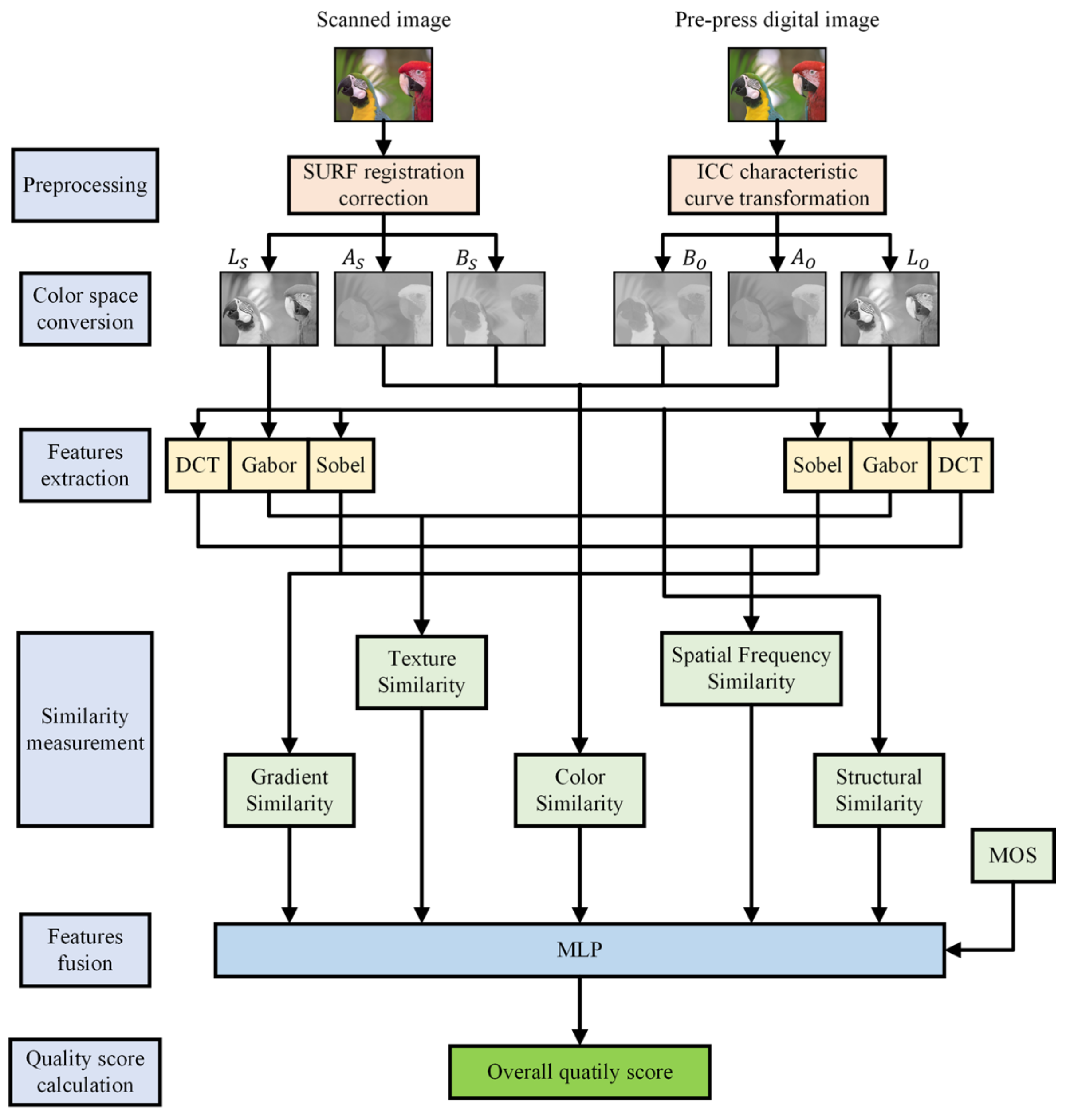
Figure 3 presents a novel metric proposed for assessing the quality of digital print images, termed Spatial-Frequency Domain Feature Fusion (FFSF). The preprocessing stage involves the feature curve transformation of pre-print digital images, wherein the images undergo processing using device ICC curves. Additionally, post-scan images undergo registration and correction. Subsequently, the preprocessed images are subjected to spatial transformation, transitioning from the original color space to the CIELAB color space. Features are then extracted from the L, A, and B channels, with chromaticity features being extracted from channels A and B. In the L channel, gradient features are computed using Sobel filters, structural features are evaluated using the structural similarity index (SSIM) metric, texture features are extracted via a Gabor filter bank, and spatial frequency features are derived by analyzing discrete cosine transform (DCT) coefficients of image blocks. Following feature extraction, similarity metrics are applied to quantify the differences between features extracted from pre-print digital images and scanned print images. Finally, an MLP neural network model trained on standard datasets is employed to predict the objective quality scores of the print images.

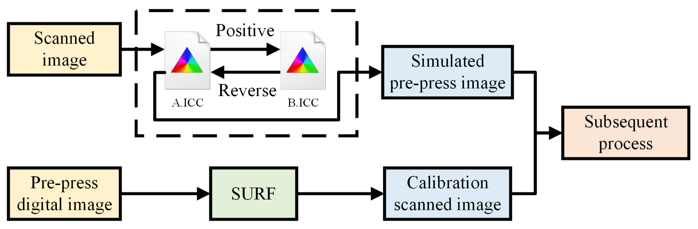
Due to inevitable issues like positional shifts and rotations during the scanning process, image registration is necessary to ensure more accurate scanned images. In this study, we utilized the SURF (Speeded-Up Robust Features) metric. Extensive research by Pang [8] has shown this metric to be highly reliable. Since the imaging principles of pre-press digital images and post-scan images differ, it is illogical to directly compare them. Spatial transformations and device characteristic curve transformations were applied to pre-press images, including both forward and inverse transformations, as depicted in Figure 4. Here, A.ICC represents the spatial transformation curve, while B.ICC denotes the device characteristic curve. The forward and reverse transformations do not preserve the original image; instead, they introduce color alterations due to the application of different ICC curves, thereby simulating the printing imaging process accurately.

For color image prints, accurately reproducing colors serves as a critical benchmark for quality control. In color image printing, challenges often arise in mapping color information between different color spaces. For instance, in digital printing, original information is typically presented in RGB or CMYK mode on a monitor, while printing involves transferring ink onto a substrate in the form of ink dots. Due to the human eye’s low-pass characteristics, it primarily perceives the overall appearance and cannot discern ink dots at a microscopic level. This underscores the essence of printing, where color gradation is manifested by the density of ink dots.

When conducting quality assessment, the selection of an appropriate color space holds significant importance in the evaluation process. We opt for the classic color space for conversion, namely the CIELAB [9,10,11] color space. If the original image is in the CMYK color space and needs to be converted to the CIELAB color space, it must first be converted to the RGB color space. However, direct conversion from the RGB color space to the CIELAB color space is not possible; instead, it necessitates the use of the XYZ color space as an intermediary. The CIELAB color space comprises a luminance channel and two chromaticity channels. The conversion formula is as follows:

$$\begin{array}{ccc}{linear}_r& =& redTRC\left[{device}_r\right]\\ {linear}_g& =& greenTRC[{device}_g]\\ {linear}_b& =& blueTRC[{device}_b]\end{array},$$

(1)

$$\begin{array}{c}\left[\begin{array}{c}{connection}_X\\ {connection}_Y\\ {connection}_Z\end{array}\right]=\\ \left[\begin{array}{ccc}{redColorant}_X& {greenColorant}_X& {blueColorant}_X\\ {redColorant}_Y& {greenColorant}_Y& {blueColorant}_Y\\ {redColorant}_Z& {greenColorant}_Z& {blueColorant}_Z\end{array}\right]\left[\begin{array}{c}{linear}_r\\ {linear}_g\\ {linear}_b\end{array}\right],\end{array}$$

(2)

$$\left\{\begin{array}{c}{L}^{*}=116f\left(\frac{{connection}_Y}{Y_n}\right)-16\\ a^{*}=500\left[f\left(\frac{{connection}_X}{X_n}\right)-f\left(\frac{{connection}_Y}{Y_n}\right)\right]\\ b^{*}=200\left[f\left(\frac{{connection}_Y}{Y_n}\right)-f\left(\frac{{connection}_Z}{Z_n}\right)\right]\end{array}\right.,$$

(3)

$$f\left(t\right)=\left\{\begin{array}{l}{t}^{\frac{1}{3}}\hspace{1em}\hspace{1em}\hspace{1em}\hspace{1em}\hspace{1em}\hspace{1em}if t>{\left(\frac{6}{29}\right)}^3\\ \frac{1}{3}{\left(\frac{29}{6}\right)}^{2}t+\frac{4}{29}\hspace{1em}\hspace{1em}otherwise\end{array}\right.,$$

(4)

Based on the device’s ICC file, the following information is obtained, including the ${redColorant}_{Tag}$, ${greenColorant}_{Tag}$, ${blueColorant}_{Tag}$, $redTRCTag$, $greenTRCTag$, and $blueTRCTag$, as shown in

Table 2. Device ICC tag sheet.

	X	Y	Z
${redColorant}_{Tag}$	0.4361	0.2225	0.0139
${greenColorant}_{Tag}$	0.3851	0.7169	0.0971
${blueColorant}_{Tag}$	0.1431	0.0606	0.7141

and Figure 5. Furthermore, it is noted that in Equation (3), $X_n,{ Y}_n$, and $Z_n$ values can be queried through the ICC file, $X_n=0.9642$, $Y_n=1.0000$, $Z_n=0.8249$.

For clarity in subsequent discussions, the following explanation is provided: The experimental objects are a preprocessed, pre-print digital image, denoted as $I_o$, and a post-scanned image, denoted as $I_s$. After color space transformation, the three-channel image information of $I_o$ includes $L_o,{ A}_o$, and $B_o$, while the three-channel image information of $I_s$ includes $L_s,{ A}_s$, and $B_s$.

2.1. Extraction of Chromaticity Features

Chroma refers to the saturation or purity of a color, indicating its intensity. Changes in chroma can reflect the accuracy and consistency of color reproduction during printing. Color features are extracted from the A and B channels. The similarity of the A channel is as follows:

$$S_c^A=\frac{1}{N}\sum _{i=1}^N\frac{2\times A_s\left(i\right)\times A_o\left(i\right)+C_1}{{A_s\left(i\right)}^2+{A_o\left(i\right)}^2+C_1},$$

(5)

In this equation, $i$ represents the index of the image pixel, and $N$ denotes the total number of pixels in the image. $C_1$ serves as a stabilizing constant for the fractional term to prevent division by zero. Similarly, the chromaticity similarity in the $B$ channel is described as follows:

$$S_c^B=\frac{1}{N}\sum _{i=1}^N\frac{2\times B_s\left(i\right)\times B_o\left(i\right)+C_1}{{B_s\left(i\right)}^2+{B_o\left(i\right)}^2+C_1},$$

(6)

The calculation of color feature similarity between $I_s$ and $I_o$ is outlined as follows:

$$S_C=\frac{1}{N}\sum _{i=1}^N\left(\frac{2\times A_s\left(i\right)\times A_o\left(i\right)+C_1}{{A_s\left(i\right)}^2+{A_o\left(i\right)}^2+C_1}\times \frac{2\times B_s\left(i\right)\times B_o\left(i\right)+C_1}{{B_s\left(i\right)}^2+{B_o\left(i\right)}^2+C_1}\right),$$

(7)

Different values of $C_1$ will lead to differences in chromaticity similarity. In order to optimize the chromaticity metrics, the TID2013 dataset was tested to judge the effect of $C_1$ values on chromaticity values via the Spearman Rank Order Correlation Coefficient (SROCC) metrics. The SROCC is used as a measure of the correlation between two variables. The SROCC value range is [−1, 1]; the closer it is to 1 or −1, the more monotonicity is achieved. The results are shown in Figure 6. Figure 6a shows the change curve of the SROCC metrics with $C_1$ taking the value of Figure 6b, which shows the change rate of the curve. From this analysis, it is concluded that the SROCC increases rapidly when the value of $C_1$ increases from 0 to about 40, which indicates that the monotonicity between the color similarity and the true value increases as the value of the parameter increases. The rate of increase of the SROCC starts to slow down when the value of $C_1$ is about 40, and enters into a smooth growth phase. When the parameter value continues to increase, the SROCC still shows a slow increasing trend, but the increase is smaller and close to linear growth. In practical applications, it may be necessary to find a balance between the performance improvement induced by the parameter value increase and the computational complexity. Too high a parameter value may not significantly improve the performance, while the computational cost will increase. All things considered, $C_1=40$ is chosen in this paper.

2.2. Gradient Features of Digital Print Images Based on the Sobel Filter

In print quality assessment, gradient refers to the rate of change in color or brightness within an image. Gradient features reveal the sharpness of edges and details, as well as variations in texture. This information is essential for evaluating print quality. Image edges play a vital role in conveying visual information, with gradient features widely utilized in image quality assessment due to their ability to capture both edge structure and contrast variations effectively [12]. Various forms of gradient features have been integrated into image quality assessment metrics. For example, the Feature Similarity Index (FSIM) incorporates gradient and phase consistency features to evaluate the local quality of distorted images [13], while the Directional Similarity Measure (DASM) combines gradient magnitude, anisotropy, and local orientation features [14,15,16,17]. Commonly employed edge detection filters include those created by Sobel, Prewitt, and Scharr [18]. The advantage of the Sobel operator lies in its robustness to noise and its relatively accurate computation of edge direction. In this study, the Sobel filter was chosen to compute the gradient of the luminance channel in both $I_o$ and $I_s$. The gradient magnitude calculation formulas for these images using the Sobel filter on the L channel are as follows:

$$G_o\left(i\right)=\sqrt{{\left(h_x\ast L_o\left(i\right)\right)}^2+{\left(h_y\ast L_o\left(i\right)\right)}^2},$$

(8)

$$G_s\left(i\right)=\sqrt{{\left(h_x\ast L_s\left(i\right)\right)}^2+{\left(h_y\ast L_s\left(i\right)\right)}^2},$$

(9)

where $G_o\left(i\right)$ and $G_s\left(i\right)$ denote the gradient magnitude values at position index $i$ of the pre-press digital image and the printed and scanned image, respectively. The symbol $\ast$ indicates the convolution operation. $h_x$ and $h_y$ represent the horizontal and vertical Sobel filter templates, defined as follows:

$$h_x=\frac{1}{4}\left[\begin{array}{ccc}1& 0& -1\\ 2& 0& -2\\ 1& 0& -1\end{array}\right], h_y=\frac{1}{4}\left[\begin{array}{ccc}1& 2& 1\\ 0& 0& 0\\ -1& -2& -1\end{array}\right],$$

(10)

The similarity between the gradient magnitudes of $I_o$ and $I_s$ is quantified using the standard deviation of the similarity:

$$G\left(i\right)=\frac{2G_o\left(i\right)\times G_s\left(i\right)+C_2}{G_o^2\left(i\right)+G_s^2\left(i\right)+C_2},$$

(11)

$$S_G=\frac{1}{N}\sum _{i=1}^{N}G\left(i\right),$$

(12)

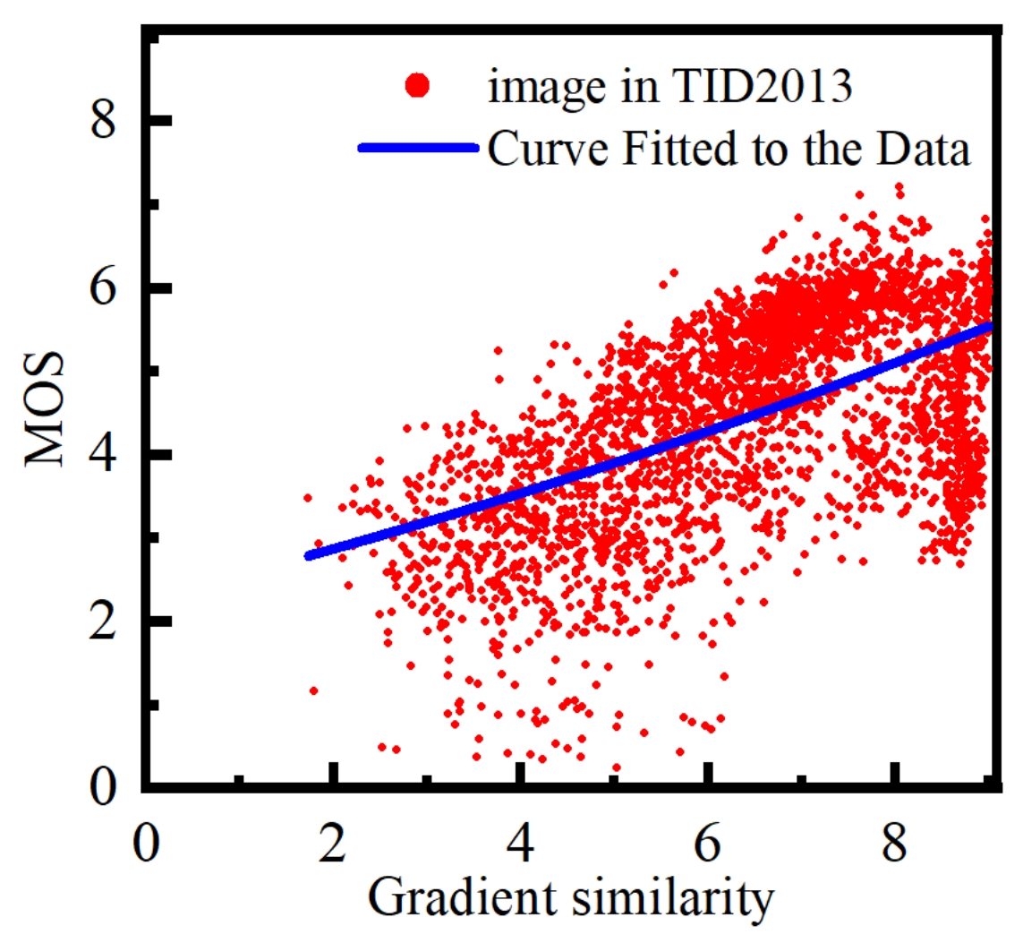
In this context, $C_2$ serves as a stabilizing constant within the fraction to prevent division by zero. The relationship strength between gradient similarity and the Mean Opinion Score (MOS) was assessed using the SROCC metric across various $C_2$ values, as illustrated in Figure 7. A higher SROCC value approaching one signifies a stronger correlation between the two datasets. Notably, the maximum SROCC value is achieved when $C_2$ is set to 66. Thus, for this study, $C_2$ is determined to be 66. The red number and dot line indicate the positions of the inflection points of the curve, which are the turning points where the curve transitions from an upward trend to a downward trend.

2.3. Printing Image Structural Features Based on the SSIM

Structure refers to the layout and organization of textures, details, and patterns within an image. The quality of structure significantly influences the visual quality of the image and the overall perception of printed materials. Based on the premise that the CIELAB color space is well suited for extracting structural information from the scene, Wang et al. [14] introduced a novel concept for measuring image quality known as the SSIM. This concept defines separate functions to measure the luminance, contrast, and structural similarity between two images, $I_o$ and $I_s$, in the L channel. Their similarity is calculated as the product of the luminance similarity $l\left(I_o, I_s\right)$, the contrast similarity $c\left(I_o,I_s\right)$, and the structural similarity $s\left(I_o,I_s\right)$, resulting in an overall measure of image similarity:

$$S_B\left(I_o, I_s\right)=l\left(I_o,I_s\right)\times c\left(I_o, I_s\right)\times s\left(I_o,I_s\right),$$

(13)

where:

$$l\left(I_o, I_s\right)=\frac{2{\mu }_{L_o}{\mu }_{L_s}+C_3}{{\left({\mu }_{L_o}\right)}^2+{\left({\mu }_{L_s}\right)}^2+C_3},$$

(14)

$$c\left(I_o, I_s\right)=\frac{2{\delta }_{L_o}{\delta }_{L_s}+C_4}{{\left({\delta }_{L_o}\right)}^2+{\left({\delta }_{L_s}\right)}^2+C_4},$$

(15)

$$s\left(I_o, I_s\right)=\frac{{\delta }_{L_o{L}_s}+C_5}{{\delta }_{L_o}{\delta }_{L_s}+C_5},$$

(16)

Let the parameters $C_4={2C}_5$, and $S_B\left(I_o, I_s\right)$ be expressed as follows:

$$S_B\left(I_o, I_s\right)=\frac{2{\mu }_{L_o}{\mu }_{L_s}+C_3}{{\left({\mu }_{L_o}\right)}^2+{\left({\mu }_{L_s}\right)}^2+C_3}·\frac{2{\delta }_{L_o{L}_s}+C_4}{{\left({\delta }_{L_o}\right)}^2+{\left({\delta }_{L_s}\right)}^2+C_4},$$

(17)

The equations demonstrate that ${\mu }_{L_o}$ and ${\mu }_{L_s}$ represent the luminance features using the mean value. Taking $L_o$ as an example, the calculation is as follows:

$${\mu }_{L_o}=\frac{1}{N}\sum _{i=1}^N{L}_o\left(i\right),$$

(18)

Similarly, the calculation for ${\mu }_{L_s}$ is as follows.

${\delta }_{L_o}$ and ${\delta }_{L_s}$ represent the contrast feature using normalized variance. For instance, the calculation for $L_o$ is as follows:

$${\delta }_{L_o}=\sqrt{\frac{1}{N-1}\sum _{i=1}^N{\left(L_o\left(i\right)-{\mu }_{L_o}\right)}^2},$$

(19)

Similarly, the calculation for ${\delta }_{L_s}$ is as follows.

${\delta }_{L_o{L}_s}$ represents the covariance used to characterize the structural feature, which is calculated as follows:

$${\delta }_{L_o{L}_s}=\frac{1}{N-1}\sum _{i=1}^N\left(L_o\left(i\right)-{\mu }_{L_o}\right)\left(L_s\left(i\right)-{\mu }_{L_s}\right),$$

(20)

$C_3={\left(k_1{L}^{\prime }\right)}^2$ and $C_4={\left(k_2{L}^{\prime }\right)}^2$ are constants employed to ensure stability. Here, $L^{\prime }$ denotes the number of grayscale levels in the image. For an 8-bit grayscale image, $L^{\prime }=255$, with $k_1=0.01,$ and $k_2=0.03$. Substituting these values, we obtain $C_3=6.5025$ and $C_4=58.5225$.

3. Extracting the Frequency Domain Features of Printed Images

3.1. Image Multiscale and Multiorientation Texture Features Based on Gabor Filters

Texture features can capture the surface structure and details of printed samples, which are crucial for evaluating the fidelity and consistency of print quality. Texture reflects certain patterns of color and grayscale variations on the surface of an object, serving as effective information to distinguish objects with similar spectral properties but different spatial distribution characteristics. It is widely used in the extraction of image information. Multiscale texture analysis methods include wavelet transform, Gabor transform, pyramid decomposition, and contourlet transform, among others. In multiscale image analysis, the support region of the Gabor filter’s main function has a rectangular structure, with its length and width varying with the scale. Therefore, it can optimally and sparsely describe the edges of an image and the approximate singular curves with the minimum number of coefficients [19].

Gabor filters can precisely adjust their response to specific orientations, making them highly effective in capturing directional information in images. Each Gabor filter is highly sensitive to local frequency components along a specific orientation. In contrast, wavelet transforms (such as Haar wavelets, Daubechies wavelets, etc.) typically have limited directional selectivity, mainly capturing horizontal, vertical, and diagonal orientations. Although extensions like 2D directional wavelets exist to provide more directional sensitivity, they are generally more complex than Gabor filters in terms of orientation control. Gabor filters are often used to simulate biological visual perception due to their similarity to the response characteristics of simple cells in the human visual system, especially in processing visual textures and edges [19,20,21,22,23]. While wavelet transforms excel in image compression and denoising, their biological relevance is typically not as strong as that of Gabor filters.

Gabor transformation can effectively analyze grayscale variations in images at various scales and orientations. A two-dimensional Gabor filter consists of a series of bandpass filters with given orientation angles and spatial frequencies. For a given frequency and orientation angle, it is defined as follows:

$$g\left(x, y, \lambda , \theta \right)=\frac{1}{2\pi {\sigma }_x{\sigma }_y}{e}^{\left[-\frac{1}{2}\left(\frac{x^2}{{\sigma }_x^2}+\frac{y^2}{{\sigma }_y^2}\right)\right]\times \left[i\left(\frac{2\pi x}{\lambda }\right)\right]},$$

(21)

In the formula

$$x=x_0\cos \theta +y_0\sin \theta ,$$

(22)

$$y={-x}_0\sin \theta +y_0\cos \theta ,$$

(23)

$\left(x_0, y_0\right)$ is the spatial position coordinate of the image pixel. $\lambda$ is the wavelength, which is the reciprocal of spatial frequency. $\theta$ is the angle between the filter orientation and the $y_0$ axis. ${\sigma }_x$ and ${\sigma }_y$ are the standard deviations of the Gaussian envelope in the $x$ and $y$ directions, calculated as follows:

$${\sigma }_x=\frac{\lambda }{\pi }\times \sqrt{\frac{\ln 2}{2}}\times \frac{2^{B_w}+1}{2^{B_w}-1},$$

(24)

$${\sigma }_y=\frac{{\sigma }_x}{\gamma },$$

(25)

where $B_w$ and $\gamma$ are the passband width and the aspect ratio of the filter frequency, respectively.

Here, $g\left(x, y, \lambda , \theta \right)$ represents a complex matrix, wherein the real and imaginary components are convolved separately with the information from $I_o$ and $I_s$ on the L channel. Subsequently, the real and imaginary parts are combined, and the modulus is calculated.

In Figure 8, we present an example of an original image extracted from the TID2013 database alongside the image’s response after being filtered by a Gabor filter bank with five scales and four orientations. From the illustration, it is evident that larger-scale filters offer superior noise reduction capabilities but may also lead to a loss of finer details.

The filters are grouped into $l$ categories based on the number of scales ($l=1,2,3,4,5$). Additionally, each scale has four orientations ($\theta =0°,45°,90°,135°$). Therefore, when computing the similarity of texture features, the weighted average of the correlation coefficients for the four orientations is calculated as follows:

$$C{C}_l\left(E_o, E_s\right)=\frac{1}{4}\sum _{\theta }\frac{\sum _{i=1}^N\left(E_s^{\theta }\left(i\right)-\overline{E_s^{\theta }}\right)·\left(E_o^{\theta }\left(i\right)-\overline{E_o^{\theta }}\right)}{\sqrt{\sum _{i=1}^N{\left(E_s^{\theta }\left(i\right)-\overline{E_s^{\theta }}\right)}^2·\sum _{i=1}^N{\left(E_o^{\theta }\left(i\right)-\overline{E_o^{\theta }}\right)}^2}},$$

(26)

where $E_o$ and $E_o$ denote the response energy of the $l-th$ scale and $\theta -degree$ Gabor filter for the pre-print digital image and the scanned image of the printed product, respectively. $\overline{E_o^{\theta }}$ and $\overline{E_s^{\theta }}$ represent the mean energies corresponding to the $\theta -degree$.

3.2. Image Spatial Frequency Characteristics Based on Discrete Cosine Transform (DCT)

Spatial frequency features reveal the distribution of various frequency components in printed samples, which helps evaluate image sharpness and detail fidelity. Contrast sensitivity is a critical visual attribute of the human visual system (HVS), where different sensitivities exist for various distortions in images. Hence, we utilize discrete cosine transform (DCT) on the luminance channel L of the image, leveraging the sub-band features derived from the image’s DCT [24,25,26,27] to emulate the contrast sensitivity function (CSF) within the HVS.

Performing 4 × 4 DCT and 8 × 8 DCT transformations on the TID2013 dataset, we calculated the spatial frequency similarity and the SROCC indicator between MOSs. The results, as shown in

Table 3. A comparison of the results for DCT variations at two scales.

	4 × 4 DCT	8 × 8 DCT
Low frequency	0.559	0.535
Mid frequency	0.595	0.510
High frequency	0.465	0.401

, indicate that the 4 × 4 transformation yields better results compared to the 8 × 8 transformation. The computation complexity of 4 × 4 DCT blocks is lower, and due to their smaller size, they can handle local changes and details in the image more accurately, especially in regions with rich, high-frequency details.

According to the research by S.-H. Bae [28], we partition the spatial frequency domain into regions with varying sensitivities to distortion. Three indicators of spatial frequency similarity are represented by comparing the contrast energy values of low-frequency (LF), mid-frequency (MF), and high-frequency (HF) regions within 4 × 4 discrete cosine transform (DCT) blocks. Figure 9 illustrates the spatial contrast sensitivity function (CSF) within the LF, MF, and HF regions of the 4 × 4 DCT blocks.

The discrete cosine transforms of two-dimensional images are as follows:

$$\begin{array}{c}F\left(u, v\right)=c\left(u\right)c\left(v\right){\displaystyle \sum _{x=0}^{M-1}}{\displaystyle \sum _{y=0}^{N-1}}f(x, y)cos\frac{\pi \left(2x+1\right)u}{2M}cos\frac{\pi \left(2y+1\right)v}{2N},\\ u=0, 1,2\dots , \mathrm{M}-1 \hspace{1em}\hspace{1em}v=0, 1,2\dots ,N-1,\end{array}$$

(27)

where

$$c\left(u\right)=\left\{\begin{array}{l}\frac{1}{\sqrt{N}}, u=0\\ \sqrt{\frac{2}{N}}, u=1,2\dots ,M-1\end{array}\right.\hspace{1em}\hspace{1em}\hspace{1em}\hspace{1em}c\left(v\right)=\left\{\begin{array}{l}\frac{1}{\sqrt{N}},v=0\\ \sqrt{\frac{2}{N}},v=1,2\dots ,N-1\end{array}\right.$$

(28)

The key advantage of two-dimensional discrete cosine transform (DCT) lies in its ability to concentrate a significant portion of the image’s energy within specific frequency ranges [25]. DCT transforms signals or images from the time domain (spatial domain) to the frequency domain [26]. This facilitates a better understanding of the frequency components present in the signal or image. In the frequency domain, one can observe the contributions of various frequency components in the signal or image, aiding in further analysis and processing.

The contrast energy map extracted from the LF region of the image is defined as described in [25]:

$${\phi }_L=\sum _{\left(u, v\right)\in R_L}{p}^2\left(u, v\right),$$

(29)

The energy calculation for the mid-frequency and high-frequency regions is computed as follows: $p(u, v)$ represents the magnitude of the DCT coefficients at $(u, v)$ and $R_L$ denotes the mid-frequency region. Similarly, the energy calculation for the mid-frequency and high-frequency regions is computed as follows:

$${\phi }_M=\sum _{\left(u, v\right)\in R_M}{p}^2\left(u, v\right),$$

(30)

$${\phi }_H=\sum _{\left(u, v\right)\in R_H}{p}^2\left(u, v\right),$$

(31)

Similar to the SSIM, the similarity index takes the form of $(2·ab+c)/(a^2+b^2+c)$. Therefore, the similarity index between $I_o$ and $I_s$ in the low-frequency domain is defined as follows:

$$S_L=\frac{1}{n}\sum _{\left(u, v\right)\in R_L}\frac{2{\phi }_{oL}·{\phi }_{sL}+C_6}{{{\phi }_{oL}}^2+{{\phi }_{sL}}^2+C_6},$$

(32)

where ${\phi }_{oL}$ and ${\phi }_{sL}$ represent the contrast energy maps of $I_o$ and $I_s$ in the low-frequency domain, respectively. $n$ denotes the number of 4 × 4 pixel blocks into which the image is divided, and $C_6$ is a constant that is used to maintain stability. Similarly, the similarity in the mid-frequency and high-frequency domains is given as follows:

$$S_M=\frac{1}{n}\sum _{\left(u, v\right)\in R_M}\frac{2{\phi }_{oM}·{\phi }_{sM}+C_7}{{{\phi }_{oM}}^2+{{\phi }_{sM}}^2+C_7},$$

(33)

$$S_H=\frac{1}{n}\sum _{\left(u, v\right)\in R_H}\frac{2{\phi }_{oH}·{\phi }_{sH}+C_8}{{{\phi }_{oH}}^2+{{\phi }_{sH}}^2+C_8},$$

(34)

where ${\phi }_{oM}$ and ${\phi }_{sM}$, respectively, represent the contrast energy maps of $I_o$ and $I_s$ in the MF region. ${\phi }_{oH}$ and ${\phi }_{sH}$, respectively, represent the contrast energy maps of $I_o$ and $I_s$ in the HF region. $n$ denotes the number of 4 × 4 pixel blocks into which the image is divided. $C_7$ and $C_8$ are two positive invariants controlling numerical stability. To determine the appropriate invariant constants, a series of tests were conducted. Various values of $C_6$, $C_7$, and $C_8$ were examined, with the SROCC used as the metric, to evaluate the relationship between the spatial frequency similarity and the MOS. As shown in Figure 10, the blue curve represents the SROCC under different invariant constant values, while the red curve indicates the rate of change of the SROCC. Figure 10a,d represent the low-frequency region, Figure 10b,e represent the mid-frequency region, and Figure 10c,f represent the high-frequency region. The results indicate that with the increase in the invariant constant, the SROCC shows an upward trend in all three regions, but the growth rate gradually decreases. This suggests that excessively high values of the invariant constant may not significantly improve performance. Considering all factors, it was concluded that the optimal values are $C_6=0.03$, $C_7=0.04$, and $C_8=0.03$.

3.3. Neural Network Regression

Machine learning serves as an effective solution for addressing regression problems, with various well-established methods proving successful in image quality assessment (IQA) regression. These methods include the k-nearest neighbor (KNN) model [30], support vector machines (SVMs) [31,32,33], random forest [34,35], and neural networks [36]. While linear regression and KNN calculations are relatively straightforward, they often encounter challenges in achieving optimal results. SVM metrics pose difficulties in their implementation, especially with large-scale training samples. The reliance of SVMs on quadratic programming for solving support vectors involves m-order matrix calculations (where m is the number of samples). When the number of samples is substantial, the storage and computation of this matrix can significantly consume machine memory and processing time.

The MLP neural network possesses powerful nonlinear fitting capabilities. Through learning, the MLP neural network can automatically adjust its internal weights, gradually adapting to different tasks and environments. This enables the neural network to exhibit excellent generalization capabilities in handling regression problems, and MLP neural networks demonstrate good robustness and fault tolerance. Based on the significant advantages of the MLP mentioned above, we chose the MLP neural network to train a regression mapping model between quality description metrics and subjective image evaluation scores.

We construct the regression function $f\left(X\right)$, which, given the input metrics, yields the final objective quality assessment score:

$$Q=f\left(S_C,S_G,S_S,{CC}_1,{CC}_2,{CC}_3,{CC}_4,{CC}_5,S_L,S_M,S_H\right),$$

(35)

The architecture of the MLP neural network is depicted in Figure 11. It consists of two hidden layers. The first hidden layer processes 11-dimensional input data and produces 64 output nodes. The second hidden layer then takes these 64 nodes and reduces them to 32 output nodes. A ReLU activation function is applied between these two hidden layers to introduce nonlinearity.

4. Experimental Results and Analysis

To assess the effectiveness of the proposed metrics, experiments were conducted on two standard databases: TID2013 [37] and TID2008 [38]. Both datasets comprise a selection of distorted images that are utilized to evaluate the perceptual quality of images. The TID2008 dataset comprises 25 reference images along with their respective distorted versions. The distortions in TID2008 encompass noise, blur, compression artifacts, and various other types of distortions. The TID2013 dataset comprises 3000 reference images paired with their corresponding distorted versions. The distortions applied to these images encompass a range of common types, including noise, blur, compression artifacts, and others. Four key performance metrics were employed for a quantitative evaluation: the Pearson Linear Correlation Coefficient (PLCC), SROCC, the Kendall Rank Order Correlation Coefficient (KROCC), and the Root Mean Square Error (RMSE). The PLCC gauges the model’s prediction accuracy, reflecting its ability to predict subjective assessments with minimal error. The RMSE measures the consistency of the model’s predictions. The SROCC and the KROCC indicate the monotonicity of the model’s predictions, showcasing how well it can predict subjective assessments. The proposed method underwent comparison with nine classical Full-Reference image quality assessment (FR-IQA) methods, including GMSD [17], GSM [16], IFC [39], MAD [40], MSSIM [41], PSNR [42], SSIM [14], VIF [43], and VSI [44].

The color space transformation is performed on both the original digital image and the scanned print image, as illustrated in Figure 12:

Using the TID2013 dataset as an example, the images in the TID2013 dataset were printed and subsequently scanned to obtain scanned images. The relationship between the chromaticity similarity index in the CIELAB space and the MOS was validated, utilizing the MOS provided by the dataset itself, according to the method described in Section 2.1. Figure 13 illustrates the distribution of the chromaticity similarity and the MOS for printed images in the CIELAB color space:

The scatter plot depicts a consistently distributed set of data points, which are densely clustered, suggesting the precision of the method outlined in Section 2.1.

Similarly, this study examines the correlation between the gradient similarity metric proposed in Section 2.2 and the MOS. Figure 14 illustrates the distribution of gradient similarity against the MOS:

The scatter plot shows a relatively uniform distribution of data points with high concentrations, indicating the accuracy of the method proposed in Section 2.2.

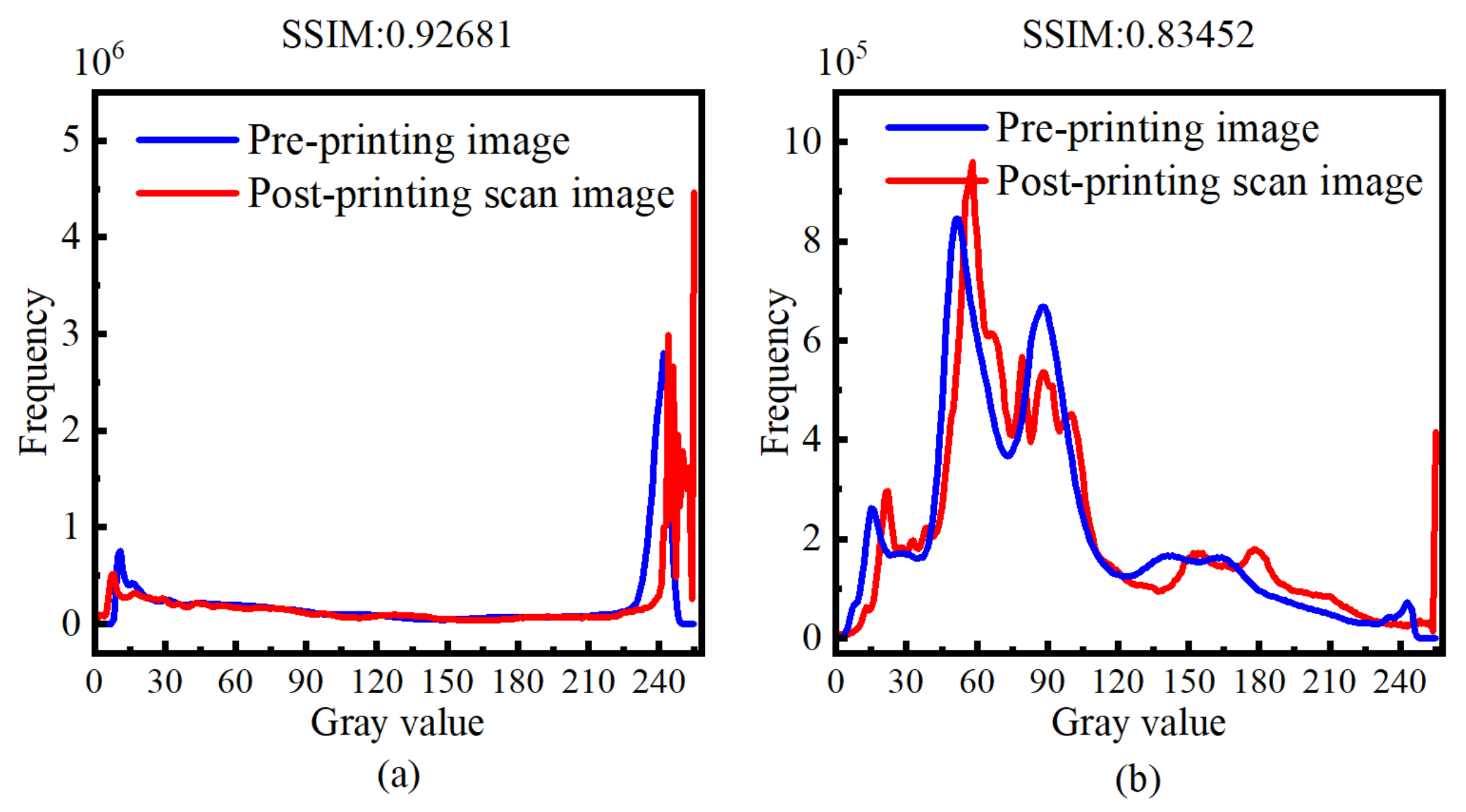
Randomly selected images from the TID2008 and TID2013 standard datasets were used to measure the SSIM values of the pre-print digital images and the scanned images, along with their energy histograms, as shown in Figure 15. It can be observed that the energy distribution of the two images is nearly identical in the low-frequency region. However, in the high-frequency region, the energy of the pre-print digital image is higher than that of the scanned image. This is because printing cannot perfectly reproduce continuous-tone images. Additionally, it can be concluded that the printing quality is poorer in the color depth region. This is reasonable because printing machines have a saturation point: once the ink density reaches a certain level, the color becomes saturated, and further increasing the ink amount will not change the color.

This paper selects features from Gabor filters with four orientations and five scales. The selection method for the orientation parameter $\theta$ is as follows:

$${\theta }_k=\frac{k\pi }{n}, k=\{0, 1, 2, \dots , n-1\},$$

(36)

Here, $n$ represents the total number of filter orientations. In this paper, we select four orientations, so the angles are, respectively, ${\theta }_0=0°$, ${\theta }_1=45°$, ${\theta }_2=90°$, ${\theta }_3=135°$.

The parameter $f$ of the Gabor filter represents the frequency of the filter, and it is calculated as follows:

$$\sigma \cdot f=\frac{1}{\pi }\sqrt{\frac{\ln 2}{2}}\times \frac{2^B+1}{2^B-1},$$

(37)

$B$ represents the bandwidth of the filter, typically set as $B=1$, then $\sigma \cdot f=0.56$. For a filter bank, its frequency can be expressed as follows:

$$f_k=a^{-k}{f}_{max},k=(0, 1, \dots , m-1),$$

(38)

$m$ represents the total number of frequencies for the filter, where $a=\sqrt{2}$. In this study, five scales are chosen, and thus $m=5$.

As shown in Figure 16, the real and imaginary parts of the Gabor filter are illustrated.

In the process of image learning, 80% of the images from each database were randomly selected for training, and the remaining 20% were used for testing. To ensure fair comparisons, the training–testing process was repeated 1000 times, and the median of the results after 1000 iterations was taken as the final outcome to eliminate performance biases. The indicators for measuring the strengths and weaknesses of the quality evaluation metrics are shown below:

• The SROCC metric evaluates the monotonic relationship between the image quality assessment metrics and the subjective evaluation, indicating whether the objective assessment maintains a consistent trend with changes in the subjective evaluation. The SROCC value ranges from −1 to 1, with values closer to 1 or −1 indicating stronger monotonicity.
• The PLCC metric assesses the linear correlation between the image quality assessment metrics and the subjective evaluation, with values ranging from −1 to 1. Positive values denote a positive correlation, negative values signify a negative correlation, and 0 indicates no correlation. The closer the absolute value is to one, the more accurate the metric’s evaluation.
• The KROCC metric measures the rank correlation between two variables, with values ranging from −1 to 1. A value close to 1 indicates a strong correlation, while a value of 0 implies independence.
• The RMSE quantifies the deviation between the image quality assessment metrics and the subjective evaluation, with smaller values indicating higher consistency. An RMSE value approaching 0 signifies the high accuracy of the metrics.

This paper compares nine commonly used FR-IQA metrics, including GMSD, GSM, IFC, MAD, MSSIM, PSNR, SSIM, VIF, and VSI.

Table 4. A performance comparison of 10 metrics on two databases.

		GMSD	GSM	IFC	MAD	MSSIM	PSNR	SSIM	VIF	VSI	FFSF
TID2013	KROCC	0.6339	0.6255	0.6785	0.7327	0.5977	0.7161	0.5588	0.6665	0.7183	0.7720
	PLCC	0.8590	0.8464	0.8791	0.9071	0.8319	0.9080	0.7895	0.8769	0.9000	0.9397
	RMSE	0.6346	0.6603	0.5905	0.5219	0.6880	0.5193	0.7608	0.5959	0.5404	0.4256
	SROCC	0.8044	0.7946	0.8697	0.9052	0.7779	0.8925	0.7417	0.8510	0.8965	0.9316
TID2008	KROCC	0.7092	0.6596	0.7009	0.7294	0.6636	0.9120	0.5758	0.6991	0.7123	0.8017
	PLCC	0.8788	0.8422	0.8810	0.8899	0.8579	0.7395	0.7732	0.8762	0.8762	0.9485
	RMSE	0.6404	0.7235	0.6349	0.6120	0.6895	0.9078	0.8511	0.6468	0.6466	0.4277
	SROCC	0.8907	0.8504	0.8903	0.9051	0.8559	0.5628	0.7749	0.8840	0.8979	0.9444

presents the results of testing these nine common metrics along with the proposed metric on two standard databases. The bolded numbers denote the evaluation metrics with the best performance. Based on the descriptions of the SROCC, PLCC, KROCC, and RMSE, combined with the data in the table, it is evident that the performance of the proposed FFSF metric is superior.

The selection of various regression methods leads to diverse evaluation outcomes. To identify a suitable regression approach for feature fusion, this section conducts a comparison between random forest (RF) and the MLP neural network. As shown in

Table 5. A performance comparison of two regression methods.

		RF	SVR	MLP
TID2013	KROCC	0.7777	0.7426	0.8452
	PLCC	0.9426	0.9180	0.9680
	RMSE	0.4095	0.6907	0.4907
	SROCC	0.9315	0.9083	0.9483
TID2018	KROCC	0.7921	0.7497	0.8197
	PLCC	0.9429	0.9159	0.9659
	RMSE	0.4422	0.6017	0.5333
	SROCC	0.8382	0.8738	0.9118

, except for the RMSE metric, the results for the remaining three metrics are all superior in the MLP compared to the RF. The results of the SVR are comparatively less favorable. Furthermore, since RMSE ranges from 0 to positive infinity, both methods fall within a similar, small range, indicating comparable performance. In summary, the evaluation metrics obtained through regression using the MLP neural network surpass those obtained using the RF. The bolded numbers denote the evaluation metrics with the best performance.

The study concurrently compared results from the same model using different loss functions. Experiments were conducted using an MLP neural network model with various loss functions, and the findings are summarized in

Table 6. MLP regression models with different loss functions.

		MAE	MSE
TID2013	KROCC	0.6974	0.8452
	PLCC	0.8637	0.9680
	RMSE	0.6784	0.4907
	SROCC	0.8745	0.9483
TID2018	KROCC	0.7619	0.8197
	PLCC	0.9031	0.9659
	RMSE	0.8769	0.5333
	SROCC	0.7697	0.9118

, showing that MSE outperforms MAE in terms of results.

To illustrate the consistency between the proposed metrics in this paper and human subjective ratings, scatter plots were generated, as shown in Figure 17. These plots display the evaluation results of nine commonly used metrics relative to the MOS in the TID2013 database. It is evident that the results obtained from individual evaluation methods exhibit considerable dispersion in the scatter distribution of image MOSs, lacking a clear trend. Further analysis through curve fitting accentuates the inconsistency between subjective and objective assessments. This outcome unequivocally indicates significant disparities between the objective quality assessment results obtained and the subjective ratings. To demonstrate the alignment between the metrics proposed in this study and human subjective ratings, scatter plots were generated, as depicted in Figure 17. These plots illustrate the evaluation outcomes of nine commonly used metrics relative to the Mean Opinion Score (MOS) in the TID2013 database. The GMSD metric shows poor monotonicity and a weak trend in the fitted curve, indicating varied GMSD scores for the same MOS. GMSD, primarily assessing image gradient magnitude similarity as an objective metric, does not fully encompass subjective image quality perception, which is influenced by factors like color, contrast, and noise. Hence, different GMSD scores may occur for identical MOS values. Similar issues are observed with the IFC metric. In contrast, GSM, MAD, MSSIM, SSIM, VIF, and VSI metrics exhibit relatively better performance, showing more pronounced growth trends in scatter plots and fitted curves. Among them, SSIM performs notably well despite its high data dispersion. Conversely, PSNR performs the least favorably, analyzing images solely from a pixel perspective and neglecting their multidimensional attributes, diverging from real-world conditions. Clearly, individual evaluation methods yield notably dispersed results in MOS scatter plots, lacking definitive trends. Further curve fitting analysis underscores the disparity between subjective and objective assessments, distinctly highlighting substantial differences between objective quality assessment results and subjective ratings.

Compared to other methods, the metrics proposed in this paper demonstrate significant advantages in their evaluation results. As shown in the scatter plot in Figure 18, the data distribution is more concentrated, and the curve fitting shows a good linear relationship. This result indicates a high level of consistency between the objective evaluation scores of the metrics proposed in this paper and the subjective scores.

Taking the TID2013 dataset as an example, Figure 19 clearly illustrates the variations in the loss functions of nine popular metrics and the metric proposed in this paper during the training of the MLP neural network.

Table 7. The loss convergence values for 10 metrics during training.

	GMSD	GSM	IFC	MAD	MSSIM	PSNR	SSIM	VIF	VSI	FFSF
LOSS	1.505	0.834	1.214	0.929	0.874	1.172	0.767	0.869	1.040	0.138

provides detailed convergence values of each loss function. Through comparative analysis, it is evident that although the loss functions of individual evaluation methods can converge, their effectiveness is not satisfactory. This indicates that a single evaluation method is insufficient to fully meet the complex requirements of printing image quality assessment. In contrast, the metrics proposed in this paper demonstrate significant advantages in the performance of the loss function. Not only is the training effect more ideal, but the final convergence values are also superior compared to other metrics.

5. Conclusions

This paper presents an effective and reliable metric for assessing the quality of printed images that closely mimic human visual perception. Compared to mainstream single-dimensional evaluation metrics, the metrics proposed in this paper offer a comprehensive evaluation of printed images from multiple dimensions, significantly improving the accuracy and reliability of the assessment. It combines spatial and frequency domain features, starting with data analysis in the CIELAB color space. In the spatial domain, it extracts color and gradient features, calculates the similarity of different features using similarity measures, and then computes structural similarity. Subsequently, it applies Gabor transform and discrete cosine transform (DCT) to the images, utilizing texture and spatial frequency features as complementary aspects of printed image quality. Multiscale and multi-directional texture features, along with spatial frequency features, are employed for a comprehensive analysis of the frequency domain information of the images, and similarity measures are used to assess similarity at the frequency domain level. Finally, an MLP neural network regression tool is utilized to train a stable model through extensive training, predicting the overall quality scores of the printed images. Extensive experiments on publicly available databases demonstrate that the selected parameters and this method highly conform to subjective perception, exhibiting high consistency with human visual characteristics.

Samples in publicly available databases may lack diversity in certain aspects, as some databases might focus primarily on specific types of prints or particular printing conditions. This limitation could result in inadequate generalization of the results to different types of prints or conditions. Future research should employ more diverse and comprehensive databases to ensure the broader applicability of the findings. Future research directions include enhancing the accuracy and robustness of evaluation models to more comprehensively reflect print quality. One promising avenue is to explore the application of deep learning and reinforcement learning in print quality assessment. For instance, convolutional neural networks (CNN) can be used to extract image features, while reinforcement learning can be employed to optimize the evaluation process. Improving the self-learning and adaptive capabilities of these models will further enhance the efficiency and effectiveness of the assessments.

References

1. Maqsood, N.; Rimašauskas, M. Influence of printing process parameters and controlled cooling effect on the quality and mechanical properties of additively manufactured CCFRPC. Compos. Commun. 2022, 35, 101338. [Google Scholar] [CrossRef]
2. Jing, X.; Astling, S.; Jessome, R.; Maggard, E.; Nelson, T.; Shaw, M.; Allebach, J.P. A general approach for assessment of print quality. Proc. SPIE 2013, 8653, 175–184. [Google Scholar] [CrossRef]
3. Eerola, T.; Lensu, L.; Kälviäinen, H.; Bovik, A.C. Study of no-reference image quality assessment algorithms on printed images. J. Electron. Imaging 2014, 23, 061106. [Google Scholar] [CrossRef]
4. Mittal, A.; Moorthy, A.K.; Bovik, A.C. No-reference image quality assessment in the spatial domain. IEEE Trans. Image Process. 2012, 21, 4695–4708. [Google Scholar] [CrossRef] [PubMed]
5. Liang, D.; Gao, X.; Lu, W.; Li, J. Deep blind image quality assessment based on multiple instance regression. Neurocomputing 2021, 431, 78–89. [Google Scholar] [CrossRef]
6. Wang, Z.; Li, Q. Information content weighting for perceptual image quality assessment. IEEE Trans. Image Process. 2010, 20, 1185–1198. [Google Scholar] [CrossRef] [PubMed]
7. ISO 12233:2023; Photography—Electronic Still Picture Imaging—Resolution and Spatial Frequency Responses. International Organization for Standardization: Geneva, Switzerland, 2023.
8. Gupta, S.; Thakur, K.; Kumar, M. 2D-human face recognition using SIFT and SURF descriptors of face’s feature regions. Vis. Comput. 2021, 37, 447–456. [Google Scholar] [CrossRef]
9. Ze, S.; Jin, Y.; Peng, L.; Huan, Z.; Jun, J. Colour space conversion model from CMYK to CIELab based on CS-WNN. Color. Technol. 2021, 137, 272–279. [Google Scholar] [CrossRef]
10. Li, Y.; Bi, Y.; Zhang, W.; Ren, J.; Chen, J. M2GF: Multi-Scale and Multi-Directional Gabor Filters for image edge detection. Appl. Sci. 2023, 13, 9409. [Google Scholar] [CrossRef]
11. Durmus, D. CIELAB color space boundaries under theoretical spectra and 99 test color samples. Color Res. Appl. 2020, 45, 796–802. [Google Scholar] [CrossRef]
12. Manikonda, S.K.; Gaonkar, D.N. Islanding detection method based on image classification technique using histogram of oriented gradient features. IET Gener. Transm. Distrib. 2020, 14, 2790–2799. [Google Scholar] [CrossRef]
13. Liu, Y.; Fan, K.; Wu, D.; Zhou, W. Filter pruning by quantifying feature similarity and entropy of feature maps. Neurocomputing 2023, 554, 126297. [Google Scholar] [CrossRef]
14. Wang, Z.; Bovik, A.C.; Sheikh, H.R.; Simoncelli, E.P. Image quality assessment: From error visibility to structural similarity. IEEE Trans. Image Process. 2004, 13, 600–612. [Google Scholar] [CrossRef] [PubMed]
15. Gu, K.; Qiao, J.; Min, X.; Yue, G.; Lin, W.; Thalmann, D. Evaluating quality of screen content images via structural variation analysis. IEEE Trans. Vis. Comput. Graph. 2018, 24, 2689–2701. [Google Scholar] [CrossRef] [PubMed]
16. Cai, Q.; Cui, G.C.; Wang, H.X. EEG-based emotion recognition using multiple kernel learning. Mach. Intell. Res. 2022, 19, 472–484. [Google Scholar] [CrossRef]
17. Xue, W.; Zhang, L.; Mou, X.; Bovik, A.C. Gradient magnitude similarity deviation: A highly efficient perceptual image quality index. IEEE Trans. Image Process. 2014, 23, 684–695. [Google Scholar] [CrossRef]
18. Pei, X.; Hong, Y.; Chen, L.; Guo, Q.; Duan, Z.; Pan, Y.; Hou, H. Robustness of machine learning to color, size change, normalization, and image enhancement on micrograph datasets with large sample differences. Mater. Des. 2023, 232, 112086. [Google Scholar] [CrossRef]
19. Zhao, X.; Tao, R.; Li, W.; Philips, W.; Liao, W. Fractional Gabor convolutional network for multisource remote sensing data classification. IEEE Trans. Geosci. Remote Sens. 2021, 60, 5503818. [Google Scholar] [CrossRef]
20. Choi, J.Y.; Lee, B. Ensemble of deep convolutional neural networks with Gabor face representations for face recognition. IEEE Trans. Image Process. 2019, 29, 3270–3281. [Google Scholar] [CrossRef]
21. Hill, P.; Achim, A.; Al-Mualla, M.E.; Bull, D. Contrast sensitivity of the wavelet, dual tree complex wavelet, curvelet, and steerable pyramid transforms. IEEE Trans. Image Process. 2016, 25, 2739–2751. [Google Scholar] [CrossRef]
22. Ni, Z.; Zeng, H.; Ma, L.; Hou, J.; Chen, J.; Ma, K.-K. A Gabor feature-based quality assessment model for the screen content images. IEEE Trans. Image Process. 2021, 27, 4516–4528. [Google Scholar] [CrossRef] [PubMed]
23. Samantaray, A.K.; Rahulkar, A. New design of adaptive Gabor wavelet filter bank for medical image retrieval. IET Image Process. 2020, 14, 679–687. [Google Scholar] [CrossRef]
24. Dua, S.; Singh, J.; Parthasarathy, H. Image forgery detection based on statistical features of block DCT coefficients. Procedia Comput. Sci. 2020, 171, 369–378. [Google Scholar] [CrossRef]
25. Yuan, Z.; Liu, D.; Zhang, X.; Wang, H.; Su, Q. DCT-based color digital image blind watermarking method with variable steps. Multimed. Tools Appl. 2020, 79, 30557–30581. [Google Scholar] [CrossRef]
26. Sharma, S.; Sharma, H.; Sharma, J.B. Artificial bee colony based perceptually tuned blind color image watermarking in hybrid LWT-DCT domain. Multimed. Tools Appl. 2021, 80, 18753–18785. [Google Scholar] [CrossRef]
27. Sawant, S.S.; Manoharan, P. Unsupervised band selection based on weighted information entropy and 3D discrete cosine transform for hyperspectral image classification. Int. J. Remote Sens. 2020, 41, 3948–3969. [Google Scholar] [CrossRef]
28. Bae, S.-H.; Kim, M. A Novel DCT-Based JND Model for Luminance Adaptation Effect in DCT Frequency. IEEE Signal Process. Lett. 2013, 20, 893–896. [Google Scholar] [CrossRef]
29. Bae, S.-H.; Kim, M. A novel image quality assessment with globally and locally consilient visual quality perception. IEEE Trans. Image Process. 2016, 25, 2392–2406. [Google Scholar] [CrossRef]
30. Tu, B.; Wang, J.; Kang, X. KNN-Based representation of superpixels for hyperspectral image classification. IEEE J. Sel. Top. Appl. Earth Obs. Remote Sens. 2018, 11, 4032–4047. [Google Scholar] [CrossRef]
31. Ding, Y.; Zhao, Y.; Zhao, X. Image quality assessment based on multi-feature extraction and synthesis with support vector regression. Signal Process. Image Commun. 2017, 54, 81–92. [Google Scholar] [CrossRef]
32. Du, S.; Yan, Y.; Ma, Y. Blind image quality assessment with the histogram sequences of high-order local derivative patterns. Digit. Signal Process. 2016, 55, 1–12. [Google Scholar] [CrossRef]
33. Narwaria, M.; Lin, W. SVD-based quality metric for image and video using machine learning. IEEE Trans. Syst. Man Cybern. B Cybern. 2012, 42, 347–364. [Google Scholar] [CrossRef]
34. Pei, S.-C.; Chen, L. Image quality assessment using human visual DOG model fused with random forest. IEEE Trans. Image Process. 2015, 24, 3282–3292. [Google Scholar] [CrossRef] [PubMed]
35. Phan, T.N.; Kuch, V.; Lehnert, L.W. Land cover classification using Google Earth Engine and random forest classifier—The role of image composition. Remote Sens. 2020, 12, 2411. [Google Scholar] [CrossRef]
36. Ertuğrul, O.F. A novel type of activation function in artificial neural networks: Trained activation function. Neural Netw. 2018, 99, 148–157. [Google Scholar] [CrossRef] [PubMed]
37. Ponomarenko, N.; Jin, L.; Ieremeiev, O.; Lukin, V.; Egiazarian, K.; Astola, J.; Vozel, B.; Chehdi, K.; Carli, M.; Battisti, F.; et al. Image database TID2013: Peculiarities, results and perspectives. Signal Process. Image Commun. 2015, 1, 55–77. [Google Scholar] [CrossRef]
38. Ponomarenko, N.; Lukin, V.; Zelensky, A.; Egiazarian, K.; Carli, M.; Battisti, F. TID2008: A database for evaluation of full-reference visual quality assessment metrics. Adv. Mod. Radioelectron. 2009, 10, 30–45. [Google Scholar]
39. Chang, H.; Zhang, Q.; Wu, Q.; Gan, Y. Perceptual image quality assessment by independent feature detector. Neurocomputing 2015, 151, 1142–1152. [Google Scholar] [CrossRef]
40. Eskicioglu, A.M.; Fisher, P.S. Image quality measures and their performance. IEEE Trans. Commun. 1995, 43, 2959–2965. [Google Scholar] [CrossRef]
41. Rajagopal, H.; Khairuddin, A.S.M.; Mokhtar, N.; Ahmad, A.; Yusof, R. Application of image quality assessment module to motion-blurred wood images for wood species identification system. Wood Sci. Technol. 2019, 53, 967–981. [Google Scholar] [CrossRef]
42. Tanchenko, A. Visual-PSNR measure of image quality. J. Vis. Commun. Image Represent. 2014, 25, 874–878. [Google Scholar] [CrossRef]
43. Hou, R.; Zhou, D.; Nie, R.; Liu, D.; Xiong, L.; Guo, Y.; Yu, C. VIF-Net: An unsupervised framework for infrared and visible image fusion. IEEE Trans. Comput. Imaging 2020, 6, 640–651. [Google Scholar] [CrossRef]
44. Zhang, L.; Shen, Y.; Li, H. VSI: A visual saliency-induced index for perceptual image quality assessment. IEEE Trans. Image Process. 2014, 23, 4270–4281. [Google Scholar] [CrossRef] [PubMed]
Figure 1. ISO 12233 test chart (partial).
Applsci 14 05986 g001
Figure 2. The modulation transfer function (MTF) of the Epson Expression 13000XL Scanner.
Applsci 14 05986 g002
Figure 3. The flow chart of the proposed metrics.
Applsci 14 05986 g003
Figure 4. Pretreatment flow chart.
Applsci 14 05986 g004
Figure 5. Tone reproduction curve.
Applsci 14 05986 g005
Figure 6. The impact of different values of C 1 on the similarity of data chromaticity: (a) the SROCC varies with the parameter C 1 , (b) the rate of change of SROCC with respect to the parameter C 1 .
Applsci 14 05986 g006
Figure 7. The impact of different values of C 2 on the similarity of data gradients.
Applsci 14 05986 g007
Figure 8. The texture information of a reference image after filtering using a Gabor filter bank in five scales.
Applsci 14 05986 g008
Figure 9. The spatial CSF in LF, MF and HF regions for a 4 × 4 DCT block (adapted from [29]): (a) the classification of frequency regions depending on the CSF obtained in [29], (b) the three frequency regions in a 4 × 4 DCT block.
Applsci 14 05986 g009
Figure 10. The impact of different invariant constants on spatial frequency similarity: (a) the SROCC in the low-frequency region, (b) the SROCC in the mid-frequency region, (c) the SROCC in the high-frequency region, (d) the growth rate of the SROCC in the low-frequency region, (e) the growth rate of the SROCC in the mid-frequency region, and (f) the growth rate of the SROCC in the high-frequency region.
Applsci 14 05986 g010
Figure 11. Diagram of the MLP neural network architecture.
Applsci 14 05986 g011
Figure 12. The visualization of the image after being transformed into the CIELAB color space: (a) The scanned print image, (b) the scanned image’s L channel, (c) the scanned image’s A channel, (d) the scanned image’s B channel, (e) the original image, (f) the original image’s L channel, (g) the original image’s A channel, and (h) the original image’s B channel.
Applsci 14 05986 g012
Figure 13. A scatter plot of the image chromaticity similarity and the MOS in the CIELAB color space.
Applsci 14 05986 g013
Figure 14. A scatter plot of the gradient similarity against the MOS for the images.
Applsci 14 05986 g014
Figure 15. Histogram of the SSIM values for the selected scanned images compared to the original images: (a) image A, (b) image B.
Applsci 14 05986 g015
Figure 16. Visualization of the Gabor filter’s kernel.
Applsci 14 05986 g016
Figure 17. A scatter plot of subjective scores versus predicted scores for objective evaluation metrics in the TID2013 database: (a) GMSD, (b) GSM, (c) IFC, (d) MAD, (e) MSSIM, (f) PSNR, (g) SSIM, (h) VIF, and (i) VSI.
Applsci 14 05986 g017
Figure 18. A scatter plot of subjective scores versus predicted scores for the FFSF evaluation metrics in the TID2013 database.
Applsci 14 05986 g018
Figure 19. The loss convergence curves for 10 metrics during training.
Applsci 14 05986 g019