A Novel Approach for Meat Quality Assessment Using an Ensemble of Compact Convolutional Neural Networks

Abstract

The rising awareness of nutritional values has led to an increase in the popularity of meat-based diets. Hence, to ensure public health, industries and consumers are focusing more on the quality and freshness of this food. Authentic meat quality assessment methods can indeed be exorbitant and catastrophic. Furthermore, it is subjective and reliant on the knowledge of specialists. Fully automated computer-aided diagnosis systems are required to eradicate the variability among experts. However, evaluating the quality of meat automatically is challenging. Deep convolutional neural networks have shown a tremendous improvement in meat quality assessment. This research intends to utilize an ensemble framework of shallow convolutional neural networks for assessing the quality and freshness of the meat. Two compact CNN architectures (ConvNet-18 and ConvNet-24) are developed, and the efficacy of the models are evaluated using two publicly available databases. Experimental findings reveal that the ConvNet-18 outperforms other state-of-the models in classifying fresh and spoiled meat with an overall accuracy of 99.4%, whereas ConvNet-24 shows a better outcome in categorizing the meat based on its freshness. This model yields an accuracy of 96.6%, which is much better compared with standard models. Furthermore, the suggested models effectively detect the quality and freshness of the meat with less complexity than the existing state-of-the art techniques.

1. Introduction

Meat is a versatile food product in people’s daily diet as it tastes delicious and contains abundant protein, fat, and vitamins, as well as other nutrients. Besides providing energy for humans, these nutrients promote microbial growth and reproduction, which accelerates the deterioration of meat. Research reveals that meat consumption is increasing annually throughout the world [1]. Beef, chicken, lamb, goat, and pork are some common meat products which can replenish microelements, such as iron, lacking in the human body. They are an indispensable food to strengthen physical function and promote metabolism. Chicken is a source of lean, low-fat protein and, hence, is healthier in comparison with other types of meat [2]. Moreover, it is less expensive, fast growing, tasty, and as a result, the most popular kind of food. Beef is rich in protein, which helps muscle growth and supports muscle mass [3]. It provides iron and essential vitamins, which aids in reducing tiredness and fatigue. Being rich in high-quality protein, vitamins, and minerals, lamb can be an excellent component of a healthy diet. It is also referred to as a vitamin B powerhouse. Pork, red-colored meat from domestic pigs, is an excellent source of zinc and other essential vitamins and minerals needed to improve the immune system.

A significant amount of health benefits from meat consumption depend on its quality. Meat quality is greatly impacted by both external and internal factors [4]. Once exposed to light, dust, and microorganisms during transportation and sales, they take on an unappetizing appearance. As meat spoils quickly, it is critical to maintain its high quality in the face of this rising demand [5]. Thus, quality is becoming increasingly important in consumers’ purchasing decisions as meat consumption rises [2]. The quality of meat is directly related to the survival and development of human beings [6]. Some consumers are even willing to pay a higher price to guarantee the quality of meat [7]. However, in recent years, many unscrupulous merchants have shown the tendency to take risks to seize the market and obtain huge profits, resulting in various quality problems. To uphold consumers’ lawful rights and interests, government agencies and the food industry ought to pay special concern to the safety and nutritional value of meat [6]. Therefore, how to test and estimate the quality of meat has become the top priority of research.

Evaluating various meat attributes to determine whether the meat is suitable for fresh consumption and preservation for a given period of time is referred to as meat quality assessment [8]. Meat has physical, biological, and chemical properties in general. Color, texture, pH, tenderness, and freshness are all meat characteristics for accessing quality. Among these factors, freshness is considered important in determining meat quality and safety [9]. This is due to the fact that consumers frequently use the external appearance of fresh meat as the primary criteria for choosing high-quality products for consumption [10]. Meat products, in general, are deemed fresh if fewer days have elapsed and stale if more days have elapsed, regardless of their actual freshness. The color of meat conveys an intuitive impression of freshness and ingredient composition. It is not only a comprehensive indicator reflecting differences, but it is also an important factor that changes as fresh meat ages. The other important quality factor is tenderness. Freshness, however, is a dynamic factor that is influenced by the processing and display conditions of the product.

There are two major techniques to evaluate meat quality: subjective and objective [11]. Subjective methods for assessing meat quality typically rely on sensory evaluation, which includes visual and eating experiences. Subjective assessment methods have the disadvantage of being heavily reliant on evaluators’ specific experience, having poor repeatability, and being difficult to quantify [12]. In contrast, objective evaluation methods are laboratory tests that assess the physical and chemical properties of meat as well as the microorganisms present [13]. Although this method yields accurate results, the meat is ruined or damaged, and the detection process is time-consuming. As a result, modern meat processing firms are struggling to meet the demand for automated processing.

As a result, the significance of systematic meat quality assessment cannot be overstated. Traditional evaluation methods were based on sensory estimation and a chemical technique that included microbial population [14]. However, when it comes to evaluating meat quality characteristics, these methods are time-consuming, destructive, inconsistent, and unstable. The lack of quick, trustworthy, and non-destructive systems for assessing meat features has hampered the quality control section of the meat industry [11]. More efficient methods are thus required in mechanized procedures to evaluate the properties, control the process, and categorize the products. Such methods could assist the slaughter industry in obtaining information about meat quality immediately after comfort sorting and prior to further use [5].

Furthermore, these methods would assist the meat industry in determining and selecting appropriate raw material processes. An imaging method has recently been used for meat quality estimation and fast recognition of quality problems on the processing line. For effective prediction of meat quality, artificial intelligence technology is employed. It also provides indispensable clinical assistance for online meat grading and evaluation. In food science, AI technology that combines sensors, processors (computers), and other components allow for non-destructive evaluation of products. Moreover the original shape and nature of the sample is maintained.

Recent studies suggest that artificial intelligence has opened a new door in image recognition and classification tasks. Detection of glaucoma classification, skin cancer, brain tumors, COVID-19 [15], Alzheimer disease [16], etc., are the notable application areas. Artificial neural networks (ANNs), convolutional neural networks (CNNs), fully connected networks, vision transformers, etc., are widely adopted models. Among the various deep models, CNNs are the most widely used. This work sets out to examine the effectiveness of shallow CNNs in detecting the quality and freshness of meat.

This work makes the following notable contributions:

i.

Evaluating the quality of meat using a suggested ConvNet-18 model.

ii.

Investigating the freshness of meat using the proposed ConvNet-24 model.

iii.

An ensemble framework based on the averaging ensemble technique is utilized for binary and multi-class classification tasks.

The rest of the paper is structured as follows: A brief review of meat quality detection using CNNs is discussed in Section 2. In Section 3, the methodology is explained. Findings and discussions are summarized in Section 4, accompanied by conclusions in Section 5.

2. Related Work

Because of the growing demand for high-quality meat products, assessing meat quality factors has become an important step in the manufacturing process. Traditional meat quality assessments are based on chemical, physical, and sensory methods that have proved to be destructive, time-consuming, laborious, and costly. As a result, a more dependable, accurate, cost-effective, and non-destructive method is desperately needed. Recently, deep learning models have been effectively employed in meat quality assessment tasks. A brief review of meat quality assessment techniques available in the literature are described as follows:

A unique method for identifying spoiled meat using semiconductor gas sensors and image processing techniques was presented by Vinda et al. [17]. The authors utilized a gas sensor array and a camera equipped with image processing that used a grey level co-occurrence matrix to detect gases released by decaying meat. The respective responses were analyzed using ANN in order to classify the degree of spoilage. The suggested technique yielded a high success rate, up to 82% accuracy. The authors concluded that the method may eventually supersede the need for human senses in the classification of meat.

Zou et al. [18] presented a one-dimensional squeeze-and-excitation residual network (1D-SE-ResNet) to build the intricate relationship between pork freshness and near-infrared spectroscopy (NIRS). The presented approach can automatically extract features from the input spectra and can be used as an end-to-end model to streamline the modeling procedure. With a classification accuracy of 93.72%, the 1D-SE-ResNet performed the best when compared to five widely used classification models. The authors concluded that the NIRS analysis technique based on deep learning provides a promising tool for pork freshness detection.

A study by Calvin et al. [2] examined CNNs’ efficacy in assessing chicken quality. Cropping, Otsu thresholding, and RGB-to-binary conversion were performed. Images of both fresh and rotten chicken meat were used to train the CNN model Ayam6Net. The authors reported that Ayam6Net yields the highest accuracy of 92.9% when compared to other CNN models (AlexNet, VGGNet, and GoogLeNet).

A machine-learning-based approach for meat freshness prediction was suggested by Bhargav et al. [19]. Two models were employed in their work to categorize the meat sample as fresh, half-fresh, and spoiled classes. The misclassification cost metric was used to assess the models’ performance. The authors concluded that the Resnet model performed relatively well in terms of the cost of misclassification and attained an accuracy of over 90%.

Li et al. [20] developed a machine learning model for beef cut classification. Both single and multiple modality features from the beef samples were employed. This resulted in a better classification model. Furthermore, an investigation of various machine learning classifiers (such as SVM, RF, and LDA) were performed. The authors concluded that the model with multiple modality feature fusion results in a prediction accuracy of above 90%.

Classification of beef quality using artificial intelligence was suggested by Jae et al. [21]. They developed an application in a client–server system for real-time purposes. The client can take a picture of beef using a mobile phone and send it to the server. Analysis of the received image to evaluate the freshness and marbling of the beef is performed on the server side. The obtained results are sent back to the client.

Nyoman et al. [22] investigated the efficacy of pre-trained CNN models for meat classification. Three different datasets were used in this work. A total of 422 images (129 of mutton, 144 of pork, and 156 of beef) were utilized. From the experimental findings, they concluded that Resnet-50 model outperforms Resnet-101 with F1-score of 95.96%.

Assessment of red meat quality using machine learning and deep learning techniques was performed in Monika et al. [23]. The presence of nitrosamine in red meat samples was identified using SVM and deep CNN models. The authors employed the transfer learning technique to investigate the performance of various deep CNN models (such as ResNet-34, ResNet-50, ResNet-101, VGG-16, VGG-19, AlexNet, and MobileNetv2). It has been concluded that the Resnet-101 model outperforms the others with the highest accuracy of 95.45% and F1-score of 96.54%.

Abdallah et al. [24] investigated the efficacy of deep learning models for beef quality classification. Beef images that include healthy and rancid ones, obtained from Kafrelsheikh University, were employed. To mitigate the data scarcity issue, a generative adversarial network was utilized. Thus, the amount of images given to the deep CNN model was greatly increased. The authors reported an overall accuracy of 96.03% with Resnet-50 model.

Ulucan et al. [25] suggested a CNN-based approach to evaluate the quality of meat. Their research intended to maintain the highest level of quality in the retail red meat sector’s open department sales service. This was accomplished by using a tray of meat cubes for an extended period of time and acquiring RGB images every two minutes. Expert data were also gathered and used as ground truth labels in parallel. Appropriate pre-processing was performed for effective extraction of features. The authors reported a better prediction result with the suggested CNN model to classify the red meat images as fresh or spoiled.

Hidayat et al. [26] classified beef, mutton, and pork images using the Resnet152V2 model. Various pre-processing techniques like augmentation, image sharpening, and image resizing were performed. Then, the discriminative features were extracted from the pre-processed images using the layered architecture of the Resnet152V2 model. The authors considered a total of 600 images with equal instances of beef, mutton, and pork images. The authors achieved an overall classification accuracy of 80%.

A majority of the prior research works have investigated the effectiveness of pre-trained models for meat classification tasks. The pre-trained models are very deep in nature. Hence, the computational complexity is high in those models. Furthermore, these deep models may take longer training time. Developing a compact model may mitigate these issues. The ensemble method shows the benefit of combining individual models to improve prediction accuracy and the generalization performance. However, limited work has been carried out to develop an ensemble model for evaluating meat quality. Motivated by recent success, a framework based on the ensemble learning of compact CNN models for meat quality assessment is developed.

3. Methodology

CNN is a subclass of deep neural network which has gained popularity in computer vision applications. It is intended to automatically and adaptively learn spatial hierarchies of image features using the backpropagation algorithm. CNN accomplishes this task by utilizing a multilayered hierarchical arrangement of various layers such as convolutional, activation, subsampling, and fully connected. The features are recognized in a hierarchical order by these layers, beginning with simple edges and progressing to complex objects. This research proposes a novel approach to assess the meat quality using an ensemble of suggested CNN models. Two compact CNN models (ConvNet-18 and ConvNet-24) are proposed for meat quality assessment. These models are meticulously designed, taking various hyperparameters into account. A brief description of the various layers employed in the compact CNNs follows:

Convolution layer: Convolution is the fundamental linear mathematical operation performed in the convolutional layer. The usage of convolutional layers in CNN mimics the organization of the human visual cortex, where a sequence of layers evaluate an input image and recognize increasingly complex information. The convolutional layer is composed of a set of kernels that work by dividing the image into small patches, termed as receptive fields. The breaking down of an image into small blocks facilitates the extraction of feature motifs. The earlier convolutional layers extract low-level features, which are then processed by later convolutional layers to retrieve higher-level patterns. The convolved output is represented in Equation (1) as follows:

$$Z(i,j)=\sum _{i=-m}^m\sum _{j=-m}^{m}I(m-i,n-j).k(i,j)+b,$$

(1)

where $I(m,n)$ is the RGB image, $k(i,j)$ is the filter, $Z(i,j)$ is the convolved output, and b is the bias term.

Rectified linear unit layer: Non-linearities are introduced into the CNN to learn the complex features in the image. This is accomplished through the use of activation functions. The ReLU activation function, defined as $R\left(Z\right)$ = $max(0,Z)$ is used commonly for non-linearity. It never saturates, and the gradient is always high. This significantly improves the training speed.

Batch normalization layer: During training, the distribution of each layer’s inputs changes as the parameters of the previous layers change. Hence, each layer needs to continuously adapt to the new distribution obtained from the previous one, and this slows down the convergence. Batch normalization overcomes this and makes the training more efficient at the same time by reducing the covariance shift within the internal layers during training. This is accomplished by a normalization of the inputs to a layer for each mini-batch.

The first step of batch normalization is to subtract the batch mean from every output value and divide it by the batch standard deviation. Let B denote a mini-batch of size m of the entire training, then the normalized activation $X_i$ is described in Equation (2) as

$$X_i=\frac{x_i-{\mu }_B}{\sqrt{{\sigma }_B^2+ϵ}},$$

(2)

where $ϵ$ is a numeric constant. ${\mu }_B$ and ${\sigma }_B^2$ represent the mini-batch mean and variance denoted in Equations (3) and (4), respectively.

$${\mu }_B=\frac{1}{m}\sum _{i=1}^m{x}_i$$

(3)

$${\sigma }_B^2=\frac{1}{m}\sum _{i=1}^m{(x_i-{\mu }_B)}^2$$

(4)

The second step uses scaling ($\gamma$) and shifting ($\beta$) parameters as mentioned in Equation (5) to allow the variables to have any mean and standard deviation,

$$y_i=\gamma X_i+\beta .$$

(5)

These scaling and shifting parameters are trainable and learned during training. Thus, batch normalization parameterizes the mean and standard deviation as trainable parameters, which makes the distribution shifts manageable during training. This results in faster convergence.

Max pooling layer: CNN achieves dimension reduction through the use of subsampling layers. These layers help to extract a set of features that are insensitive to translational shifts and minor distortions. Reduced feature map size not only regulates network complexity but also aids in increasing generalization by reducing overfitting. Max pooling employs a kernel size of $2\times 2$ to lessen the spatial dimension and, thus, the computation time. It is used to shrink the dimensions of the feature maps in the suggested model. Thus, it greatly reduces the number of learnable parameters and the amount of computation performed in the network. The max pooling operation is performed by applying a max filter to non-overlapping subregions of the input representation. For a feature map having dimensions $n_{Ho}\times n_{Wo}\times n_{Co}$, the dimension of output feature map is $n_{Hop}\times n_{Wop}\times n_{Cop}$ and is represented by Equations (6) and (7), respectively.

$$n_{Hop}=\left[\frac{n_{Ho}-f}{S}+1\right],$$

(6)

$$n_{Wop}=\left[\frac{n_{Wo}-f}{S}+1\right],$$

(7)

where f is the pool size and S indicates the stride.

Fully connected layer: The fully connected layer combines the low- and high-level features which are extracted from the hierarchical arrangement of convolutional and max pooling layers. In general, it is a feed forward network, where the neurons from each stage connect to every neuron in the next stage. The output of the fully connected layer denotes the number of classes.

Softmax layer: This layer incorporates the softmax activation function. It normalizes the output of the fully connected layer. It is used to map the output of a neuron to a probability distribution over predicted output classes. Mathematically, it can be represented by Equation (8)

$$Sof{\left(Z\right)}_i=\frac{e^{Z_i}}{{\sum }_{k=1}^c{e}^{Z_k}},$$

(8)

where c denotes number of classes, Z is the vector, and $Sof{\left(Z\right)}_i$ indicates class probabilities.

Classification layer: The final layer in the CNN model is the classification layer. It computes the cross entropy loss between the predicted and actual output values using Equation (9).

$$loss=-\sum _{i=1}^S\sum _{j=1}^C{t}_{ij}ln\left(y_{ij}\right),$$

(9)

where S is the number of samples, C is the number of classes, $t_{ij}$ indicates the $i^{th}$ sample belongs to $j^{th}$ class, and $y_{ij}$ gives the output for sample i for class j.

3.1. ConvNet-18

An eighteen-layered CNN model (ConvNet-18) is proposed for a two-class meat quality assessment task. Figure 1 illustrates the architectural details of the suggested CNN. It utilizes four convolutional layers (CL1, CL2, CL3, and CL4), two max pooling layers (PL1 and PL2), and one fully connected layer (FCL). The initial input layer accepts the meat images for further processing. To make the computation faster, the input images are resized to $64\times 64$.

Table 1. Layer details of the proposed CNN architecture.

Layer	Number of Feature Maps	Stride	Activation Shape	Number of Trainable Parameters
Input	3	-	$64\times 64\times 3$	0
CL1	96	1	$64\times 64\times 96$	2688
BNL1	96	-	$64\times 64\times 96$	192
RL1	96	-	$64\times 64\times 96$	-
PL1	96	2	$32\times 32\times 96$	-
CL2	96	1	$32\times 32\times 96$	83,040
BNL2	96	-	$32\times 32\times 96$	192
RL2	96	-	$32\times 32\times 96$	-
PL2	96	2	$16\times 16\times 96$	-
CL3	96	1	$16\times 16\times 96$	83,040
BNL3	96	-	$16\times 16\times 96$	192
RL3	96	-	$16\times 16\times 96$	-
CL4	96	1	$16\times 16\times 96$	83,040
BNL4	96	-	$16\times 16\times 96$	192
RL4	96	-	$16\times 16\times 96$	-
FCL	-	-	$1\times 1\times 2$	49,152
Softmax	-	-	$1\times 1\times 2$	-
Classification	-	-	-	-

provides the complete details of the suggested model. The size of the first layer (input layer) is $64\times 64\times 3$, where each dimension represents height, width, and number of channels, respectively. Kernel sizes of $3\times 3\times 1$, $3\times 3\times 96$, $3\times 3\times 96$, and $3\times 3\times 96$ are used to extract the features in the first, second, third, and fourth convolutional layers, respectively. A total of ninety-six filters are used in all the convolutional layers. To preserve the spatial resolution, a stride value of one and the same padding is used in all the convolutional layers. A max pooling operation is performed in the fifth and ninth layers with a pool size $2\times 2$, stride of two, and padding of one. The output feature map from the fifteenth layer is fully connected with 8192 neurons in the fully connected layer. A softmax classifier used in the seventeenth layer computes the probability scores. The classification layer performs the classification of fresh and spoiled meat images.

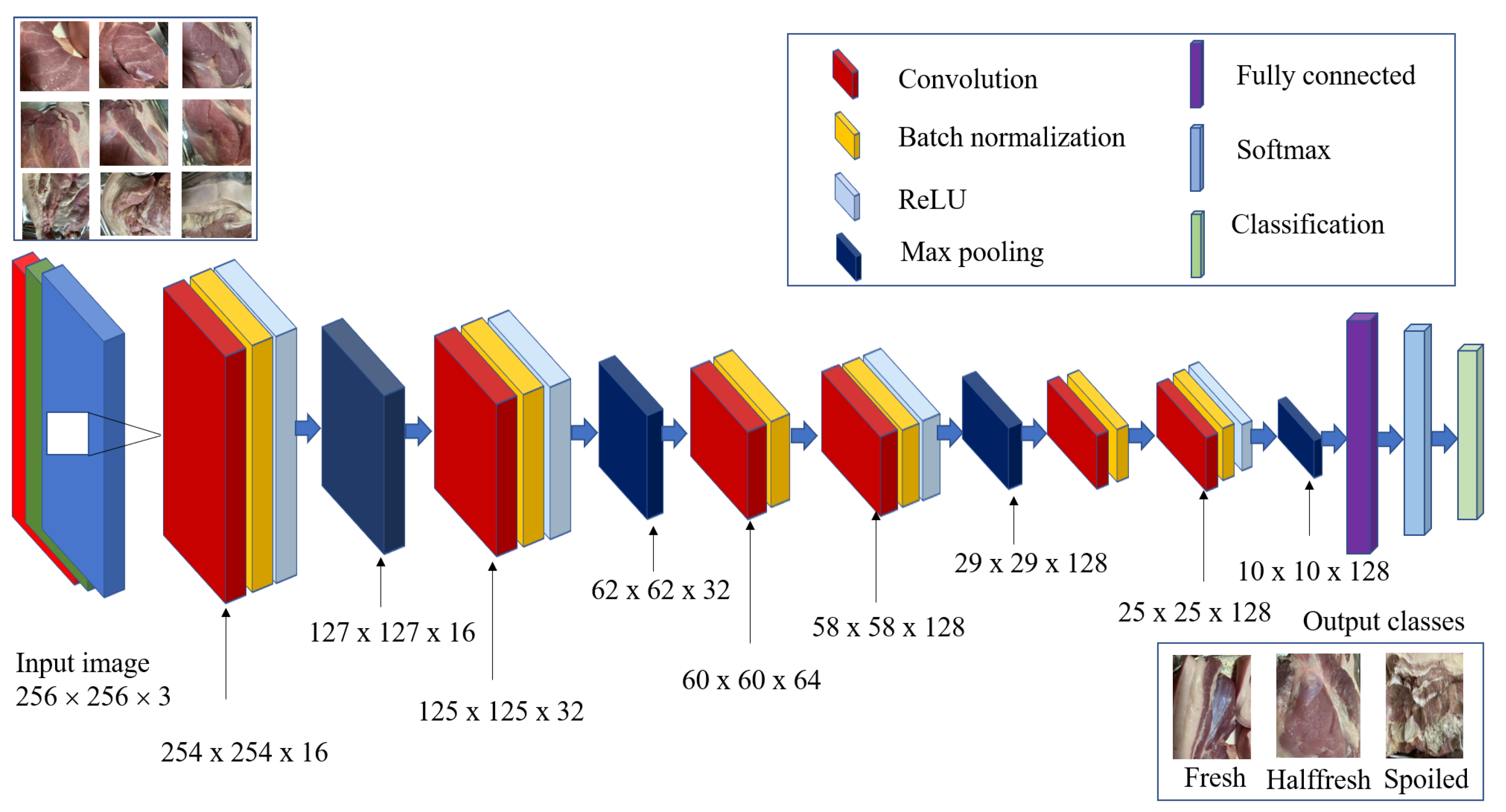
3.2. ConvNet-24

For a multi-class meat classification task, a twenty-four-layered CNN model (ConvNet-24) is proposed in this work. Figure 2 illustrates the architectural details of the suggested CNN. It includes six convolutional layers (CL1, CL2, CL3, CL4, CL5, and CL6), four max pooling layers (PL1, PL2, PL3, and PL4), and one fully connected layer (FCL). Two kernel sizes $3\times 3$ and $5\times 5$ have been used for convolution.

The entire details of the suggested ConvNet-24 is provided in

Table 2. Layer information of the ConvNet-24.

Layer	Feature Maps	Stride	Activation Shape	Trainable Parameters
Input	1	-	$256\times 256\times 3$	0
CL1	16	1	$254\times 254\times 16$	160
BNL1	16	-	$254\times 254\times 16$	32
RL1	16	-	$254\times 254\times 16$	-
PL1	16	2	$127\times 127\times 16$	-
CL2	32	1	$125\times 125\times 32$	4640
BNL2	32	-	$125\times 125\times 32$	64
RL2	32	-	$125\times 125\times 32$	-
PL2	32	2	$62\times 62\times 32$	-
CL3	64	1	$60\times 60\times 64$	18,496
BNL3	64	-	$60\times 60\times 64$	128
CL4	128	1	$58\times 58\times 128$	73,856
BNL4	128	-	$58\times 58\times 128$	256
RL4	128	-	$58\times 58\times 128$	-
PL4	128	2	$29\times 29\times 128$	-
CL5	128	1	$25\times 25\times 128$	409,728
BNL5	128	-	$25\times 25\times 128$	256
CL6	128	1	$21\times 21\times 128$	409,728
BNL6	128	-	$21\times 21\times 128$	256
RL6	128	-	$21\times 21\times 128$	-
PL6	128	2	$10\times 10\times 128$	-
FCL	-	-	$1\times 1\times 2$	76,806
Softmax	-	-	$1\times 1\times 2$	-
Classification	-	-	-	-

. The input layer accepts an image of dimension $64\times 64\times 3$. This facilitates faster computation with reduced parameters. Convolution operation is performed in the second layer with sixteen $3\times 3\times 3$ kernels and stride = 1, which results in an output map of size $254\times 254\times 16$. Batch normalization and ReLU are employed in the third and fourth layers, respectively. A max pooling operation with pool size $2\times 2$, stride = 2, and padding = 0 is performed in the fifth layer. The resultant feature map $127\times 127\times 16$ is convolved with thirty-two $3\times 3\times 32$ kernels with stride = 1 in the sixth layer, resulting in the output dimension of $125\times 125\times 32$. This is followed by batch normalization and ReLU in the seventh and eigth layers, respectively. In the ninth layer, a max pooling operation is performed over a $2\times 2$, with stride = 2 and padding = 0. This gives a feature map of dimension $62\times 62\times 32$. Again, the distinct features are extracted by convolving the feature map with sixty four $3\times 3\times 64$ kernels in the tenth layer. This gives an output of dimension $60\times 60\times 64$. Batch normalization is employed in the eleventh layer. Then, a convolution operation with one hundred and twenty eight $3\times 3\times 128$ kernels, batch normalization, and ReLU are applied on the feature map in layers twelve, thirteen, and fourteen, respectively, to produce a total of $58\times 58\times 128$ neurons. This is followed by a max pooling operation to yield a feature map of $29\times 29\times 128$ in the fifteenth layer. Again, the distinct features are extracted by convolving the feature map with one hundred and twenty-eight $5\times 5\times 128$ kernels in the sixteenth layer. This gives an output of dimension $25\times 25\times 128$. Batch normalization is employed in the seventeenth layer. Then, a convolution operation with one hundred and twenty eight $5\times 5\times 128$ kernels, batch normalization, and ReLU are applied on the feature map in layers eighteen, nineteen, and twenty, respectively, to produce $21\times 21\times 128$ number of neurons. This is followed by a max pooling operation to yield a feature map of $10\times 10\times 128$ in the twenty-first layer. The neurons are fully connected to 76,806 neurons in the twenty-second layer. A softmax classifier with cross-entropy loss function is applied in the successive layer seventeen. Finally, the classification of fresh, half fresh, and spoiled meat images are performed in the classification layer.

4. Results and Discussions

The databases employed in this study, experimental findings, and comparison with existing models are included in this section.

4.1. Meat Quality Databases

This work is experimented on two publicly available databases for assessing meat quality. The first database has two classes. The images were obtained from a supermarket in Izmir, Turkey. The goal of this database is to facilitate a collaboration between Izmir University of Economics and industry [25]. This dataset was compiled in order to create a deep-learning-based meat quality assessment system. Images were captured using an IP camera and had a resolution of $1280\times 720$. A total of 1896 images with equal instances of fresh and spoiled red meat samples are included in this dataset. Figure 3 depicts the sample images from the database. Spoiled meat images have lower pixel intensities when compared to fresh red meat images . This color characteristics can be effectively detected by deep CNN models.

The second database employed in this work is a multi-class meat freshness database [27]. The data include 1815 training images and 451 validation images. All images are of red meats, with a dimension of $416\times 416$. The images are categorized into fresh, half-fresh, and spoiled classes. The sample images are depicted in Figure 4. The distribution is largely concentrated on the brighter pixels (255) for fresh meats, while the distribution is concentrated on the dark pixels (0) for the spoiled meats. Half-fresh meat also has a more concentrated distribution on the lighter pixels than spoiled meats. These differences in pixel intensity distribution can be effectively captured by the suggested ConvNet-24 model. For convenience, the terminology MEAT2C and MEAT3C are utilized in this paper to represent the two-class and multi-class meat quality datasets.

4.2. Experimental Findings

In general, the complexity of the CNN model mainly depends on the depth of the network and number of learnable parameters involved. In this study, two shallow CNN models (ConvNet-18 and ConvNet-24) are developed to extract the primitive characteristics from meat images. Classification of meat images into fresh and spoiled classes is performed by ConvNet-18, whereas multi-class classification is performed by ConvNet-24. Both the models are implemented and investigated in three configurations (Conf1, Conf2, and Conf3). Each configuration differs in the type of optimizer employed for updating the learnable parameters. The Adam, SGDM, and RmsProp optimizers are used in Conf1, Conf2, and Conf3, respectively. In all configurations, models are trained with 80% of images and tested with unseen 20% of the images. Performance metrics such as classification accuracy (Acc), sensitivity, specificity, precision, and F-1 score are used to evaluate the efficacy of models. The description of the metrics are discussed below.

Accuracy: It is the ratio of the number of correct predictions to total predictions and is represented in Equation (10) as

$$Accuracy\left(Acc\right)=\frac{tp+tn}{tp+tn+fp+fn},$$

(10)

where $tp$ is the true positives which represent the number of fresh meat images correctly predicted by the model. True negatives ($tn$) denote the number of spoiled meat images correctly identified by the model. The number of spoiled meat images misclassified as fresh meat by the model is denoted by false positives ($fp$). The term $fn$ represents false negatives, which is defined as the number of fresh meat images mispredicted as spoiled meat by the model.

Sensitivity: It refers to the percentage of fresh meat images correctly identified by the algorithm. It is given in Equation (11) as

$$Sensitivity\left(Sen\right)=\frac{tp}{tp+fn}.$$

(11)

Specificity: It is the ratio of true negatives to the sum of true negatives and false positives. It represents the percentage of spoiled meat images correctly identified by the algorithm. It is defined in Equation (12) as

$$Specificity\left(Spe\right)=\frac{tn}{tn+fp}.$$

(12)

Precision: It indicates the ratio of correct predictions to all predictions for a particular class and is given by Equation (13)

$$Precision\left(Pre\right)=\frac{tp}{tp+fp}.$$

(13)

F1-score: It represents the harmonic mean between precision and sensitivity and is defined in Equation (14) as

$$\mathit{F}1\text{-}\mathit{score}=\frac{2\times Recall\times Precision}{Recall+Precision}.$$

(14)

These metrics are computed from the confusion matrix, and Figure 5 depicts the sample confusion matrix obtained by the ConvNet-18 model. The numbers inside green box represents true positives and true negatives. False positives and false negatives are represented inside the pink color boxes.

Proper selection of the hyperparameters allows us to achieve faster convergence. For the selection of initial learning rate and batch size, a two-stage tuning method [28] is used in this work. The model can converge or diverge if the initial learning rate is too small or too high. Therefore, for the various values of the initial learning rate (1 × 10^$-2$ to 1 × 10^$-9$), the model classification accuracy is noted in the first stage. When the initial learning rate ranges from 1 × 10^$-3$ to 1 × 10^$-5$, the results improve. In the second stage, an appropriate batch size is determined. Different batch sizes are used, including 16, 32, 64, and 100. Performance metrics are noted for each batch size by varying the initial values of the learning rate (1 × 10^$-3$ to 1 × 10^$-5$). The classification of fresh and spoiled meat images is better with a batch size equal to 32 and an initial learning rate of 1 × 10^$-3$. A batch size of 32 and an initial learning rate of 1 × 10^$-4$ produces better results for the multi-class classification task.

4.2.1. Binary Classification

The compact ConvNet-18 is trained and tested with images from both original and augmented MEAT2C database. The suggested model correctly predicts 183 among 190 fresh meat images, resulting in a sensitivity of 96.31%. Among 190 spoiled images, 180 are correctly classified by the model. Thus, an overall accuracy of 95.52% is obtained for original database. The model may fail to capture the distinct features from meat images. To enhance the overall performance of model, the amount of images is increased. This is achieved by the oversampling data level technique. The images in the original database are rotated with appropriate step size to generate the augmented database. It includes 10,428 fresh and 10,428 spoiled images.

ConvNet-18 is trained and tested with the augmented database in three different configurations.

Table 3. Performance metrics obtained using ConvNet-18.

Performance Metrics/ Configurations	Acc	Sen	Spe	Pre	F1-Score	Training Time in s	Testing Time in s
Conf1	99.6	100	99.1	99.1	99.5	1949.26	37.62
Conf2	99.4	99.8	99	99	99.4	1956.34	38.12
Conf3	99.3	99.7	98.9	99	99.3	1945.81	37.2
Ensem	99.4	99.8	99	99	99.4	5860.91	115.24

indicates the metrics obtained by ConvNet-18. It is inferred that Conf1 yields an accuracy of 99.6% by correctly predicting 2086 fresh images and 2068 spoiled images. In Conf2, a total of 4149 out of 4172 images are identified by the model. This results in an accuracy of 99.4%. When the model parameters are updated using RmsProp optimizer in Conf3, 2080 fresh and 2065 spoiled meat images are correctly predicted. This yields an accuracy of 99.3%. The robustness of the model may be improved with the ensemble technique. This work employs the average ensemble technique, where the metrics obtained by the three configurations are averaged. It is evident from experimental findings that the final ensemble model yields an accuracy of 99.43%, sensitivity of 99.8%, specificity of 99%, precision of 99%, and F1-score of 99.4% .

4.2.2. Multi-Class Classification

Classification of red meat images into fresh, half-fresh, and spoiled is performed by ConvNet-24. The efficacy of the model is investigated on both original and augmented MEAT3C database. An overall classification accuracy of 94.2% is reported when the model is evaluated on the original database. The performance may be improved for the larger dataset. Hence, the training images are enlarged using rotation augmentation technique, whereas the testing images are unaltered. With this augmented dataset, the model is trained and tested in various configurations.

Table 4. Performance metrics obtained using ConvNet-24.

Configurations/ Performance Metrics	Acc	${\mathit{Sen}}_{\mathit{M}}$	${\mathit{Pre}}_{\mathit{M}}$	$\mathit{F}\mathbf{1}\mathbf{\text{-}}{\mathit{Score}}_{\mathit{M}}$	Training Time in s	Testing Time in s
Conf1	96.5	96.7	96.4	96.5	202.34	7.61
Conf2	96	96.4	95.9	96.1	204.56	7.86
Conf3	97.3	97.5	97.1	97.3	201.87	7.42
Ensem	96.6	96.8	96.5	96.6	615.27	16.28

depicts the metrics obtained by the ConvNet-24 model. The macro-average sensitivity $Se{n}_M$ [29] is computed by summing the sensitivity of individual classes and is given by Equation (15).

$$Se{n}_M=\frac{{\sum }_{i=1}^N\frac{t{p}_i}{t{p}_i+f{n}_i}}{N}$$

(15)

The percentage of fresh meat images correctly identified is denoted by $Se{n}_F$. $Se{n}_{HF}$ and $Se{n}_{SP}$ indicate the percentage of half-fresh and spoiled meat images identified correctly by the model. The mathematical equations for computing the sensitivity is defined in Equations (16)–(18) as follows:

$$Se{n}_F=\frac{t{p}_{Fresh}}{t{p}_{Fresh}+t{n}_{Fresh}},$$

(16)

where $t{n}_{Fresh}$ denotes false negatives of the fresh class. It can be computed by adding the number of fresh samples that the model incorrectly identified as half-fresh and spoiled classes

$$Se{n}_{HF}=\frac{t{p}_{HalfFresh}}{t{p}_{HalfFresh}+t{n}_{HalfFresh}},$$

(17)

where $t{n}_{HalfFresh}$ is false negatives of the half-fresh class. It can be computed by adding the number of half-fresh samples that the model misclassified as fresh and spoiled classes:

$$Se{n}_{SP}=\frac{t{p}_{Spoiled}}{t{p}_{Spoiled}+t{n}_{Spoiled}},$$

(18)

where $t{n}_{Spoiled}$ is false negatives of the spoiled classes. It can be computed by adding the number of spoiled samples that the model misclassified as fresh and half-fresh classes. The macro-average precision $Pr{e}_M$ is computed by summing the precision of individual classes and is given in Equation (19) as

$$Pr{e}_M=\frac{{\sum }_{i=1}^N\frac{t{p}_i}{t{p}_i+f{p}_i}}{N},$$

(19)

The precision of individual classes is represented as $Pr{e}_F$, $Pr{e}_{HF}$, and $Pr{e}_{SP}$ which are computed using the equations defined in Equations (20)–(22):

$$Pr{e}_F=\frac{t{p}_{Fresh}}{t{p}_{Fresh}+f{p}_{Fresh}},$$

(20)

where $f{p}_{Fresh}$ is false positives of the fresh class. It can be computed by adding the number of half-fresh and spoiled samples that the model misclassified as fresh class.

$$Pr{e}_{HF}=\frac{t{p}_{HalfFresh}}{t{p}_{HalfFresh}+f{p}_{HalfFresh}},$$

(21)

where, $f{p}_{HalfFresh}$ is false positives of the half-fresh class. It can be computed by adding the number of fresh and spoiled samples that the model misclassified as half fresh class.

$$Pr{e}_{SP}=\frac{t{p}_{Spoiled}}{t{p}_{Spoiled}+f{p}_{Spoiled}},$$

(22)

where, $f{p}_{Spoiled}$ is false positives of the spoiled classes. It can be computed by adding the number of fresh and half-fresh samples that the model misclassified as spoiled class.

The macro-average F-score $F1\text{-}scor{e}_M$ is computed using Equation (23)

$$F1\text{-}scor{e}_M=\frac{2\ast Se{n}_M\ast Pr{e}_M}{Se{n}_M+Pr{e}_M},$$

(23)

Figure 6 depicts the confusion matrix obtained by ConvNet-24 model. True positives and true negatives are indicated inside the green color box. The numbers inside pink box represents false negatives and false positives.

From the experimental findings, it is evident that Conf1 correctly classifies 170 fresh meat images, 152 half-fresh meat images, and 113 spoiled meat images. This results in an overall accuracy of 96.5%. The sensitivities of fresh, half-fresh, and spoiled classes are found to be 95.5%, 95.6%, and 99.1%, respectively. The precision of fresh, half-fresh, and spoiled cases in Conf1 is 97.7%, 95 and 96.5%, respectively. In Conf2, 433 of 451 images are correctly identified, resulting in an accuracy of 96%. This configuration yields a sensitivity of 94.4%, 95.6%, and 99.1% in fresh, half-fresh, and spoiled cases, respectively. The precision of fresh, half-fresh, and spoiled cases is found to be 97.6%, 93.8%, and 96.5%, respectively. Among 178 fresh meat images, 172 images are correctly predicted in Conf3. This configuration predicts 154 half-fresh and 113 spoiled meat images correctly. This leads to an accuracy of 97.3%. $Se{n}_F$, $Se{n}_{HF}$, and $Se{n}_{SP}$ are found to be 96.6%, 96.8%, and 99.1%, respectively. This configuration results in a precision of 98.8%, 96.2%, and 96.5% in fresh, half-fresh, and spoiled classes, respectively. Ensembling the models can improve the overall performance [30]. Furthermore, it improves the robustness. This work employs the average ensemble technique, where the metrics obtained by the three configurations are averaged. Thus, the final ensemble model yields an overall accuracy of 96.6%.

4.3. Comparison with Pre-Trained Models

Several pre-trained models such as (Alexnet, Mobilenet-V2, Resnet-50, VGG-16, VGG-19, Densenet-201, and Efficientnet-b0) are implemented in this work. These models are customized for binary and three-class classification tasks. Faster and easier training is critical. To accomplish this, transfer learning is employed. For all pre-trained models, the initial layers and weights are transferred. Modification is performed in the final layers. Stochastic gradient descent with momentum (SGDM) optimizer is used to update the learnable parameters. An initial learning rate of 1 × 10^$-4$ and a batch size of 32 are selected. A brief description of pre-trained models follows:

Alexnet: It is regarded as the first deep CNN architecture capable of producing better outcomes for image classification tasks. The inclusion of deeper layers and various parameter optimization strategies have significantly improved the architecture’s learning capacity [31]. The major downside of the deeper network is overfitting. This issue is tackled by arbitrarily skipping some transformational units during the training phase.

VGG-16 and VGG-19: Two standard deeper neural networks (VGG-16 and VGG-19) [32] are developed by the Visual Geometry Group (VGG) from Oxford University to explore the influence of network depth on classification accuracy. With a kernel size of $3\times 3$, image features are extracted for better classification.

Resnet-50: The performance of deeper networks may become saturated or even degraded due to the vanishing gradient problem. Residual networks are developed primarily to tackle the degradation issue encountered in deeper networks [33]. This is accomplished by incorporating residual connections (previous layer outputs connected to new layer outputs) into the network.

Mobilenet-v2: The cornerstone of this architecture is an inverted residual block, which comprises three layers [34]. The expansion layer uses $1\times 1$ kernel to expand the number of channels with an appropriate expansion factor. The second layer performs the depth-wise convolution using $3\times 3$ kernels. Finally, the spatially filtered feature map is projected to low-dimensional space using a projection layer ($1\times 1$ convolution). Furthermore, a residual connection is added to aid the gradient flow during backpropagation.

Densenet-201: It comprises four dense blocks and three transition blocks [35]. Each dense block has varying number of dense layers (6, 12, 48, 32 in blocks 1, 2, 3, 4, respecitvely) which are densely connected. The network can be thinner and compact, as each layer receives feature maps from all proceeding layers.

Efficientnet-b0: Efficientnet architecture incorporates the compound scaling method to uniformly scale network width, depth, and resolution [36]. It uses inverted bottleneck convolution, which consists of a layer that first expands the network and then compresses the channels. Instead of using the ReLU activation function, this model uses a new activation function, swish activation. Compared to the various models (b0–b7), Efficientnet-b0 requires fewer parameters.

Table 5. Performance metrics obtained by various pre-trained models on MEAT2C database.

Performance Metrics/ Network	Acc	Sen	Spe	Pre	F1-Score	Training Time in s	Testing Time in s
Alexnet	98.8	98.9	98.7	98.7	98.8	7571.08	54.13
Mobilenet-V2	99.3	99.7	98.4	98.9	99.3	12,907.56	86.7
Resnet-50	99.8	99.9	99.7	99.7	99.7	14,951.2	98.76
VGG-16	99.2	99.7	98.8	98.8	99.2	16,950.6	357.92
VGG-19	99.8	100	99.6	99.6	99.8	18,804.4	361.25
Densenet-201	99.6	100	99.1	99.1	99.5	199,074.8	230.78
Efficientnet-b0	99.4	99.7	99	99	99.3	14,192.24	123.06

describes the metrics obtained by various pre-trained models for a binary classification task. Experimental findings reveal that majority of the pre-trained models perform better in classifying fresh and spoiled meat images. Though Alexnet yields an accuracy of 98.8%, it can be trained faster compared to other models. Densenet-201 takes a longer training time compared to other models. The highest classification accuracy is obtained by the Resnet-50 and VGG-19 models.

Table 6. Performance metrics obtained by various pre-trained models on MEAT3C database.

Performance Metrics/ Network	Acc	${\mathit{Sen}}_{\mathit{M}}$	${\mathit{Pre}}_{\mathit{M}}$	$\mathit{F}\mathbf{1}\mathbf{\text{-}}{\mathit{Score}}_{\mathit{M}}$	Training Time in s	Testing Time in s
Alexnet	96	96.4	96	96.2	935.45	4.14
Mobilenet-V2	94.7	95	95	95	2945.67	8.17
Resnet-50	96.7	97	96.6	96.8	5991.25	9.88
VGG-16	95.8	96	95.7	95.8	8706.6	34.92
VGG-19	97.1	97.2	96.9	97	11,239.8	36.17
Densenet-201	94.5	95	94.5	94.7	20,832.4	20.28
Efficientnet-b0	96.8	97	96.7	96.8	5506.23	11.07

represents the metrics obtained by various pre-trained models for multi-class classification. Experimental findings reveal that VGG-19 outperforms the other models in classifying the meat images into three different classes. This model correctly predicts 172 fresh meat images. Among 159 half-fresh images, 154 are correctly classified. Also, this model predicts 112 of 114 spoiled images correctly. This results in an overall accuracy of 97.1%.

Table 7. Details about different CNN models.

Network	Number of Layers	Input Size	Parameters (in Millions)
Alexnet	25	$227\times 227$	61
VGG-16	41	$224\times 224$	138.3
VGG-19	47	$224\times 224$	143.6
Resnet-50	177	$224\times 224$	25.5
Mobilenet-v2	155	$224\times 224$	3.5
Densenet-201	708	$224\times 224$	20
Efficientnet-b0	290	$224\times 224$	5.3
EnsemConvNet-18	18	$64\times 64$	0.301
EnsemConvNet-24	24	$256\times 256$	0.956

depicts the number of layers, input size, and number of learnable parameters in different CNN models considered in this work. EnsemConvNet-18 and EnsemConvNet-24 represents the ensemble of ConvNet-18 and ConvNet-24, respectively. It is evident that the total number of learnable parameters in the suggested models is less compared with other state-of-the-art architectures.

5. Conclusions

A deep ensemble framework based on the averaging ensemble technique for binary and multi-class classification of meat images is presented in this paper. At first, two compact CNN models (ConvNet-18 and ConvNet-24) are developed and investigated in various configurations for meat classification. Two publicly available databases (such as MEAT2C and MEAT3C) are employed in this work. The effectiveness of ConvNet-18 is investigated on the MEAT2C dataset, whereas the efficacy of ConvNet-24 is evaluated on the MEAT3C database. Experimental findings reveal that ensembling the various configurations of the suggested ConvNet-18 results in an overall accuracy of 99.4% in classifying fresh and spoiled meat images. The ensemble ConvNet-24 model yields a better classification accuracy of 96.6% towards classifying fresh, half-fresh, and spoiled meat images. This study also reveals that the suggested shallow CNN models can effectively classify the meat images with reduced computations compared with other state-of-art models. Furthermore, the suggested ensemble framework may greatly improve the overall performance of the meat classification task.