An Innovative Deep Learning Futures Price Prediction Method with Fast and Strong Generalization and High-Accuracy Research

Abstract

Futures commodity prices are affected by many factors, and traditional forecasting methods require close attention from professionals and suffer from high subjectivity, slowness, and low forecasting accuracy. In this paper, we propose a new method for predicting the fluctuation in futures commodity prices accurately. We solve the problem of the slow convergence of ordinary artificial bee colony algorithms by introducing a population chaotic mapping initialization operator and use the resulting chaotic mapping artificial bee colony algorithm as a trainer to learn long short-term memory neural network hyperparameters. With the combination of gate structures learned by the algorithm, the long short-term memory network can accurately characterize the basic rules of futures market prices. Finally, we conduct a series of backtesting experiments on gold and natural gas futures commodity prices to demonstrate the effectiveness of the proposed model. The experimental results show that, compared with various existing optimization models, our proposed model is able to obtain the lowest mean absolute error, mean square error, and root mean square error in the least number of iterations. In summary, the model can be used to predict the prices of a wide range of futures commodities.

1. Introduction

Predicting commodities prices in the futures market has always been a classic and challenging problem that has an impact on many countries and even the whole world [1]. Economists and computer scientists are interested in predicting futures commodity prices in economic market research [2,3]. Known for its extensive hedging capabilities and stable value, gold holds a prominent place in the investment and financial markets. The development and export of the natural gas industry play a key role in the economic growth of many countries, and natural gas exports can generate significant foreign exchange earnings for the country. Forecasts suggest that natural gas is poised to supersede coal and oil as the predominant fossil fuel post-2030 in terms of its share of the world’s primary energy consumption [4,5]. The world economy, geopolitics, inflation, and other factors all have an impact on commodities futures. Therefore, when predicting the value of these futures commodities, traditional methods require careful attention to market dynamics and relevant macroeconomic data. At the same time, researchers also face the challenge of improving the accuracy of futures commodity price volatility prediction models, as improving predictive performance is crucial for related companies and stakeholders [6]. For the investor to grasp futures commodity prices in advance of the day before the opening of the market so that they can decide whether to continue to buy or sell, thereby affecting the return on the capital, it is crucial to design an accurate forecasting model to predict commodity price trends.

During exploration and exploitation, the ABC optimization algorithm can easily slip into local optima due to its poor convergence speed [7,8]. Simultaneously, optimizing neural network hyperparameters for the faster training of high-precision prediction models is another complicated issue. Hyperparameter adjustments take a large amount of time in traditional methods, and even minor alterations can exert a huge impact on the outcome of the prediction [9,10]. In this paper, we propose a novel approach for enhancing the ABC technique by introducing a chaotic bee colony initialization operator. This operator can speed up the optimization process and be used as a hyperparameter selection for LSTM neural networks. The overarching objective is to automatically adjust the LSTM neural network’s numerous combinations of hyperparameters when forecasting various futures commodities, allowing the model to withstand market fluctuations better and adjust to changing market trends. The significance of hyperparameters in neural network training is emphasized in much research. For instance, Chen et al. [11] claim that choosing the right hyperparameters is primarily responsible for the LSTM’s performance. Similarly, Qi et al. [12] contend that hyperparameters wield substantial influence over machine learning algorithms, and that optimizing them can be computationally costly. They suggest using a Q-learning approach to find optimal neural network hyperparameter setups. Moreover, the hyperparameter exploration LSTM predictor (HELP), a superior stochastic exploration technique introduced by Li et al. [13], further corroborates the profound impact of LSTM hyperparameters on neural network performance. Furthermore, Albahli et al. [14] employ advanced techniques for hyperparameter adjustment to evaluate model efficacy, demonstrating how neural network hyperparameters affect the recognition of handwritten digits.

The originality of this study lies in its innovative use of a tent chaotic mapping artificial bee colony (TCM-ABC) technique to optimize the hyperparameters of LSTM neural networks, including critical parameters such as window size and neuron count. By harnessing the capabilities of the ABC algorithm, this study endeavors to find robust LSTM hyperparameters within vast decision spaces, thus enabling the effective training of neural networks for the precise prediction of futures commodity prices. Overall, the salient characteristics of this pioneering approach can be summarized as follows:

• Employing the globally optimized chaotic mapping artificial bee colony algorithm, this study endeavors to tune essential LSTM layer hyperparameters such as window size and neuron count.
• TCM-ABC-LSTM is a new combination of meta-heuristic algorithm and neural network, deployed for the precise prediction of daily closing prices in gold and natural gas futures commodities markets.
• By contrasting the anticipated closing price with actual values and forecasts based on statistical error measurements (such as MSE, MAE, and RMSE), the proposed TCM-ABC-LSTM model is assessed.
• To our best knowledge, this is the first time that machine learning technology has been used to predict commodity price fluctuations in the futures market.

This paper is organized as follows: Section 2 reviews past research related to our work. Section 3 describes the deep learning algorithms used in our study and our proposed TCM-ABC-LSTM architecture. Section 4 describes the experiment and discussion, including an introduction to the equipment used, data description and preprocessing, model parameter settings, results, and discussion. Section 5 concludes.

2. Related Works

Financial forecasting involves a diverse array of methodologies because the futures market, and indeed the entire financial market, are dynamic systems rife with noise and non-parameters [15]. A variety of models have been used by researchers to forecast price volatility. Four key types of price prediction methods currently in use include statistical methods, artificial intelligence methods, hybrid models, and Bayesian methods. As a result, the applications of numerous methods in the field of financial forecasting are briefly reviewed in this section.

2.1. Using Statistical Methods to Predict

Over the preceding decades, the autoregressive integrated moving average (ARIMA) model has emerged as a cornerstone within the domain of time series forecasting, garnering widespread acclaim across diverse disciplines. Predicting issues in the fields of medicine, engineering, social sciences, stocks, and futures are among its uses [16,17,18,19,20]. One of the most popular classical econometric methods for time series prediction is multiple linear regression. Multiple linear regression was employed by Jyothi Manoj et al. [21] to forecast gold prices. Ruslan et al. [22] used a series of univariate GARCH models to examine oil prices and shipping stock prices in 2021, and the study provides a realistic view for regulators and investors to predict market sentiment in the shipping market in response to global oil prices. Wahyuny et al. [23] analyzed the comparison of the accuracy of the asset pricing model (CAPM) and the arbitrage pricing theory (APT) in predicting the stock returns of manufacturing companies listed on the Indonesian stock exchange, where the outcomes of the data analysis demonstrated that the CAPM model outperforms the APT model in predicting stock returns.

2.2. Using Artificial Intelligence Methods to Predict

Artificial intelligence methods, including machine learning and deep learning methods, have been introduced and used to predict time series [24]. In 2020, Wang and Zhao [25] developed, tested, and validated suitable support vector regression (SVR) models for ship price prediction based on the advantages of support vector machine frameworks. They pointed out that this model provides satisfactory, robust, and promising results. Yu and Yan [26] used a deep neural network for predicting stock prices, which uses the time series phase space reconstruction (PSR) method to reconstruct the price series, and they claimed that the proposed prediction model has high prediction accuracy. In order to predict the opening price, the minimum price, and the maximum price of a stock at the same time, Guangyu Ding and Liangxi Qin designed a multiple-input–output model based on LSTM and experimentally demonstrated that the model outperforms other models in predicting multiple values at the same time [27]. To extract and forecast future properties of these markets, Ehsan et al. [28] suggested a CNN-based framework that can be applied to datasets from many sources (including different marketplaces). Wang et al. [29] used the most recent deep learning framework, the Transformer model, in 2022 to predict stock market indices. They showed that the Transformer model outperforms other neural network methods in multiple stock indices and better characterizes the fundamental rules of the stock market thanks to its encoder–decoder architecture and multi-head attention mechanism.

2.3. Using Hybrid Models to Predict

To predict the Bitcoin price, Kazeminia et al. proposed a hybrid model that mixes a 2D-CNN and LSTM in 2023, using a 2D-CNN for feature extraction and giving it to LSTM for prediction [30]. The results show that the hybrid model can outperform any single deep learning model. Lu et al. [31] suggested a convolutional neural network (CNN)- and LSTM-based stock price prediction technique in 2020. Effective information was extracted from the data using the CNN, and the extracted features were predicted using LSTM. According to the results, the model has the best prediction accuracy on the Shanghai Stock Exchange composite index. In 2021, Farah et al. [32] proposed a new genetic long short-term memory framework consisting of long short-term memory and a genetic algorithm to predict short-term wind power generation. The LSTM layer’s window size and neuron count were optimized using the genetic algorithm’s global optimization technique. The model is 30% more accurate than the current technology. In 2022, Gourav et al. [33] proposed a hybrid deep learning model based on an LSTM network and adaptive particle swarm optimization (PSO), which uses PSO to evolve the weights and biases of LSTM and a fully connected layer (FCL) for predicting the short-term and long-term stock prices of Sensex, S&P 500, and Nifty 50 stock indices. Compared with the Elman neural network and standard LSTM neural network, it achieved better prediction accuracy.

2.4. Using Bayesian Methods to Predict

In 2020, Massari [34] examined the impact of the market choice hypothesis on the accuracy of the probabilities implied by equilibrium prices and on the market’s “learning” mechanism, using the standard machinery of dynamic general equilibrium models to generate a rich class of price probabilities, and showed that Bayes’ rule is the only rational way to learn. A major limitation of traditional deep learning is the quantification of uncertainty in predictions, which can affect investor confidence. To this end, Chandra et al. [35] used a new Bayesian neural network to forecast multi-stage stock prices before and during the New Crown Pneumonia in 2021. The results show that the Bayesian neural network can provide reasonable forecasts with uncertainty quantification, despite the high market volatility during the first peak of the new crown pneumonia pandemic. Chuang and Lee [36] empirically analyzed historical block data using a Gaussian process model and compare its performance with GasStation-Express and the Geth gas price oracles. The results show that the Gaussian process model provides better estimates when trading volumes are volatile.

3. Methodology

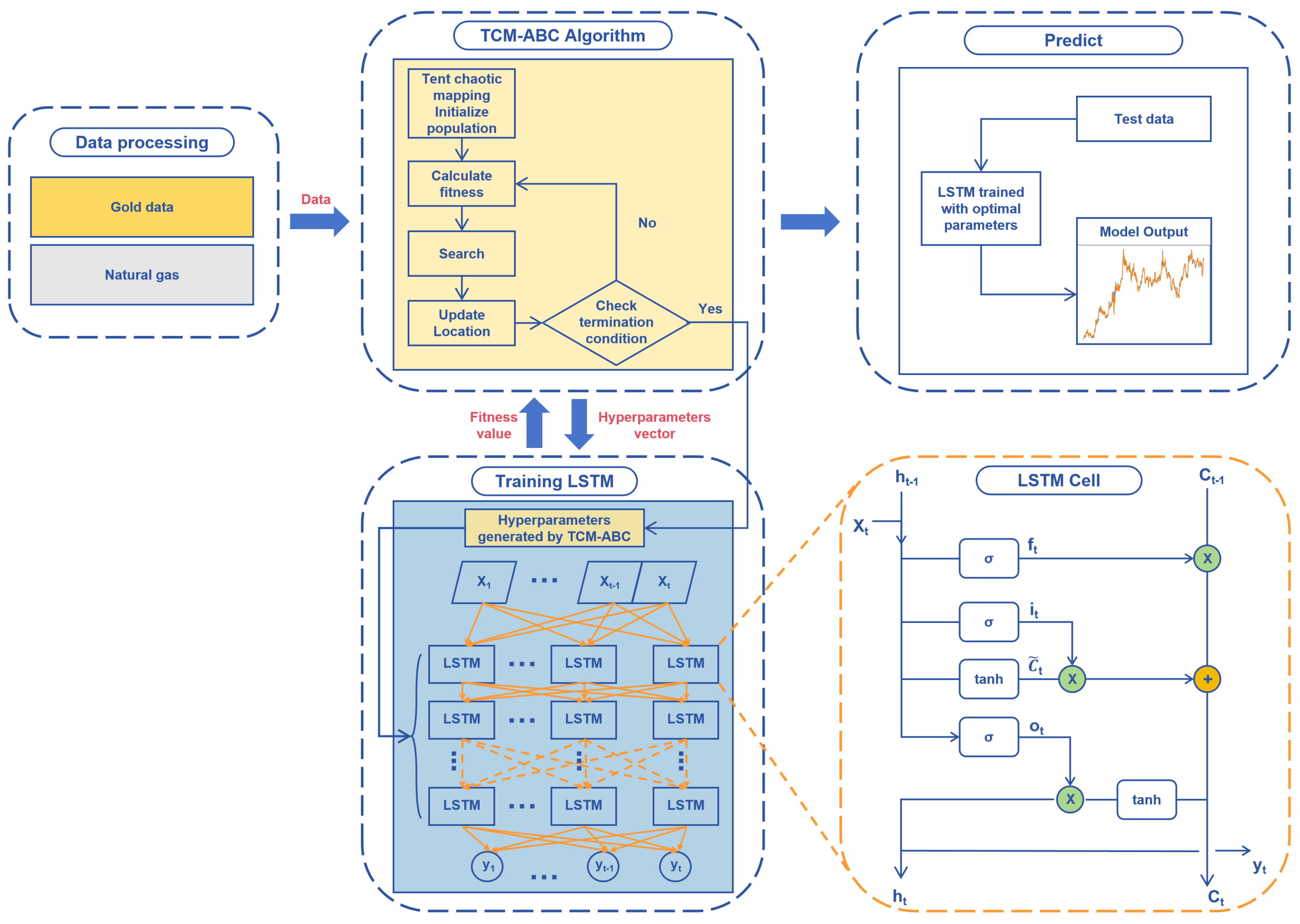
In our study, we enhance the conventional artificial swarm meta-heuristic algorithm by introducing a novel swarm initialization operator, which uses a chaotic mapping algorithm to generate the initial population, and by applying this algorithm to generate optimal hyperparameters for long short-term memory neural networks. Our primary objective is to employ this optimized model to forecast the prices of gold and natural gas futures. This section provides a comprehensive exposition of our model architecture and the methodological approaches employed therein. Figure 1 shows the created TCM-ABC-LSTM model.

Figure 1. TCM-ABC-LSTM model structure. The data are first preprocessed and divided into training and testing sets. The training set is input into TCM-ABC for training. TCM-ABC continuously generates LSTM hyperparameter vectors to train the LSTM model, and the prediction accuracy of the LSTM model is returned as fitness to TCM-ABC. Finally, the LSTM model is trained using the optimal hyperparameter vector obtained after meeting the termination conditions, and predictions are made.

3.1. Tent Chaotic Mapping Artificial Bee Colony Algorithm

The artificial bee colony (ABC) algorithm is an effective optimization algorithm that is a natural heuristic algorithm proposed by Karaboga D et al. in 2005 [37]. Functioning akin to the organic processes observed within bee colonies, the ABC categorizes bees into three distinct groups: worker bees, onlooker bees, and scout bees.

However, despite its efficacy, the algorithm for the ABC remains subject to continual refinement. The conventional approach for the ABC is to create worker bee placements in the solution space at random to start the bee population. We found that the traditional ABC algorithm’s randomly initialized bee colonies may be too concentrated, leading to poor performance. Therefore, in our research, we use tent chaotic mapping as the bee colony initialization operator, which effectively solves the inherent inefficiency problem of this traditional method [38].

Our proposed initialization operator markedly reduces exploration time by systematically distributing worker bees across the solution space. This strategy results in shorter distances for worker bee exploration, consequently enhancing search speed and efficiency. Equation (1) provides the representation of tent chaotic mapping, where $\mu$ is typically 2. We iteratively generate a series of chaotic numbers through Equation (2) and map the generated chaotic sequence $x_0,x_1,\dots ,x_n$ to the search space of the problem in Equation (3), where $x_{ij}$ represents the jth component of the current solution vector for worker bee i and $[a,b]$ is the solution space. The symbol $\lfloor \rfloor$ denotes downward rounding.

$$T\left(x\right)=\left\{\begin{array}{cc}\mu x\hfill & ,0\le x<\mu \hfill \\ \mu (1-x)\hfill & ,\mu \le x\le 1.\hfill \end{array}\right.$$

(1)

$$x_{n+1}=T\left(x_n\right)$$

(2)

$$x_{ij}=a_j+\lfloor x_i\ast (b_j-a_j)\rfloor$$

(3)

We use the mapping results obtained from the above steps as the initial population for the artificial bee colony algorithm. The fitness value of the objective function $fit$ is calculated by Equation (4), where $f_i$ is the objective function value and $fi{t}_i$ is the fitness of bee i.

$$fi{t}_i=\frac{1}{1+f_i}$$

(4)

We use the roulette method to calculate the probability $p_i$ that a worker bee is selected by an onlooker bee, which is obtained from Equation (5):

$$p_i=\frac{f_i}{{\sum }_{i=1}^{n}fi{t}_i}$$

(5)

Onlooker bees searching for new solutions are calculated using Equation (6), where $x_{kj}$ is the solution vector of a randomly selected other worker bee k.

$$x_{ij}^{\prime }=x_{ij}+rand[-1,1](x_{ij}-x_{kj})$$

(6)

Scouter bees use Equation (7) to randomly generate new solutions to avoid falling into local optima, where $x_{ij}^{″}$ is the position of the scouter bee and $x_j^{min}$ and $x_j^{max}$ represent the minimum and maximum of the jth component, respectively.

$$x_{ij}^{″}=x_j^{min}+rand[-1,1](x_j^{max}-x_j^{min})$$

(7)

3.2. Long Short-Term Memory

The long short-term memory network stands as a seminal and highly effective model for time series prediction [39]. The memory cell of the LSTM model is shown in Figure 2. The LSTM model incorporates a sophisticated gate structure to mitigate the challenges of gradient vanishing and explosion. This gate structure comprises forget gates, input gates, and output gates, and each structure has its unique role. Three gate structures are represented mathematically by Equations (8)–(11):

$$f_t=\sigma (W_f{x}_t+W_{hf}{h}_{t-1}+b_f)$$

(8)

$$i_t=\sigma (W_i{x}_t+W_{hi}{h}_{t-1}+b_i)$$

(9)

$$o_t=\sigma (W_o{x}_t+W_{ho}{h}_{t-1}+b_o)$$

(10)

$$h_t=tanh\left(C_{t-1}\right)⨂o_t$$

(11)

$$C_t=C_{t-1}⨂f_t+tanh(W_C{x}_t+W_{hC}{h}_{t-1}+b_C)⨂i_t$$

(12)

Figure 2. LSTM memory cell structure.

In Equations (8)–(12), matrices $w_{xf}$, $w_{xi}$, $w_{xo}$, $w_{xc}$ denote the appropriate input weight matrices, $w_{hf}$, $w_{hi}$, $w_{ho}$, $w_{hc}$ are the recursive weight matrices, and $b_f$, $b_i$, $b_o$, $b_c$ denote the corresponding bias vectors. The hidden state, denoted by the $h_t$ in Equation (11), passes through the activation function tanh to produce a new hidden state after combining the input and the previous hidden state into a vector. Long-term memory is represented by $C_t$, which is the outcome of the input gate, forget gate, and memory $C_{t-1}$ from the previous moment combined. The symbol ⨂ represents the multiplication of elements by elements between units. The tanh and sigmoid kernel functions are represented as tanh and $\sigma$, respectively, and are defined mathematically as follows:

$$tanh\left(x\right)=\frac{e^x-e^{-x}}{e^x+e^{-x}}$$

(13)

$$\sigma \left(x\right)=\frac{1}{1+e^{-x}}$$

(14)

The output $y_t$ of the LSTM is computed using Equation (15), where $w_{hy}$ is the recursive weight matrix and $b_y$ is the corresponding bias vector:

$$y_t=\sigma (w_{hy}{h}_t+b_y)$$

(15)

3.3. TCM-ABC-LSTM

To better address the difficulties associated with hyperparameter tuning in LSTM networks, this section describes an improved artificial bee colony optimization algorithm as a hyperparameter selector for LSTM networks, which is called TCM-ABC-LSTM. Leveraging the inherent strengths of the ABC algorithm as a hyperparameter selector, our proposed methodology ensures expedited convergence, heightened prediction accuracy, and enhanced robustness of the resultant LSTM network models. Notably, the ABC algorithm’s aptitude for tackling NP-hard problems and swiftly identifying global optimal solutions or approximate global optima highlights its effectiveness in the complex environment of hyperparametric optimization. Tent chaotic mapping group initialization further improves the efficiency of the algorithm, allowing it to quickly traverse the solution space and find the global optimal or near-global-optimal solution faster than other meta-heuristic algorithms. The pseudo-code of the TCM-ABC algorithm is shown in Algorithm 1.

Algorithm 1 Pseudocode of TCM-ABC-LSTM

1: Initialize population using Tent chaotic mapping 2: Evaluate the fitness of the population 3: Set Iteration = 1 4: while Iteration < Maximum number of Iteration do 5:       Employee Bee Phase 6:       Probability Calculation Phase 7:       Onlooker Bee Phase 8:       Scout Bee Phase 9:       Enroll the best solution obtained so far 10:      Iteration = Iteration + 1 11: end while 12: Training LSTM with Optimal Population

First, the ABC initializes the worker bee population by tent chaotic mapping (TCM), which serves to distribute the population uniformly in the solution space, to accelerate the bee’s search process and to avoid falling into local optima. The pseudo-code of the TCM initialization operator is shown in Algorithm 2.

Algorithm 2 Pseudocode of TCM initialization operator

1: while i = 1, 2,…,n do 2:     while j = 1, 2,…,m do 3:           Initialize population of worker bees W by Equations (1)–(3) 4:     end while 5: end while

In the worker bee phase following the initialization process, the worker bee evaluates the fitness value of the newly generated nectar source. Under the support of the TCM initialization operator, the searchability of the solution is enhanced. The described bee phase is demonstrated in Algorithm 3.

Algorithm 3 Worker Bee Phase

1: for all worker bee w in W do 2:       Evaluate the fitness of w 3: end for

In the onlooker bee phase, worker bees share information about the location of the nectar source with onlooker bees in the beehive. The onlooker bee selects the worker bee to continue exploring the new solution based on the roulette probability. The pseudo-code for this process is represented in Algorithm 4:

Algorithm 4 Onlooker Bee Phase

1: for all worker bee w in W do 2:      Execute roulette selection based on Equation (5) 3:       if w selected then 4:           Add w to O 5:       end if 6: end for 7: for all onlooker bee o in O do 8:       Generate $o_{new}$ by fine-tuning the value of o 9:       Evaluate the fitness of $o_{new}$ 10:       if $f\left(o\right)<f\left(o_{new}\right)$ then 11:           Replace o with $o_{new}$ 12:       end if 13: end for

Finally, the ABC enters the Scout Bee Phase if the adaptation does not improve after n iterations, replacing the current solution with a randomly generated one to avoid falling into a local optimum. We argue that the behavior of bees in the ABC algorithm has some similarities with LSTM neural network parameter tuning and that the behavior of worker bees exploiting a nectar source corresponds to finding a solution within the hyperparametric feasible solution space of the neural network. Onlooker bees can decide whether to exploit or not and are capable of small-scale fine-tuning. The scout bees randomly search for nectar sources and are able to prevent falling into a local optimum. Therefore, we choose to combine the ABC algorithm with LSTM in an attempt to achieve excellent prediction results.

TCM-ABC is used to train LSTM networks to solve nonlinear regression (predicting price fluctuations). The main difficulty in developing accurate neural network models lies in finding the most appropriate hyperparameters to train the neural network. The main drawbacks of traditional training algorithms include local optimum stagnation, slow convergence, and poor accuracy, thus motivating researchers to look for reliable alternatives to address these drawbacks. From this point of view, TCM-ABC intelligently chooses the hyperparameters of LSTM. The proposed model uses LSTM as the objective function of TCM-ABC and evaluates its solution in the training phase. This evaluation uses the current solution as hyperparameters, passes it to the LSTM, and subsequently calculates the fitness based on the predictive performance of the LSTM. This scenario is repeated until the maximum number of iterations is reached. The best solution is finally passed to the LSTM as a hyperparameter vector for the testing phase.

Using an improved artificial bee colony technique, we were able to determine the hidden layer size, number of hidden layers, time step, batch size, and epoch of LSTM in our work. Determining these ideal settings is crucial since, for instance, if the time step size is set to 1, hardly any information is transmitted. If we consider a large time step, then this means that early-sequence terms will act as noise. Thus, the appropriate optimization of these hyperparameters is indispensable for ensuring the efficacy and reliability of LSTM network models. 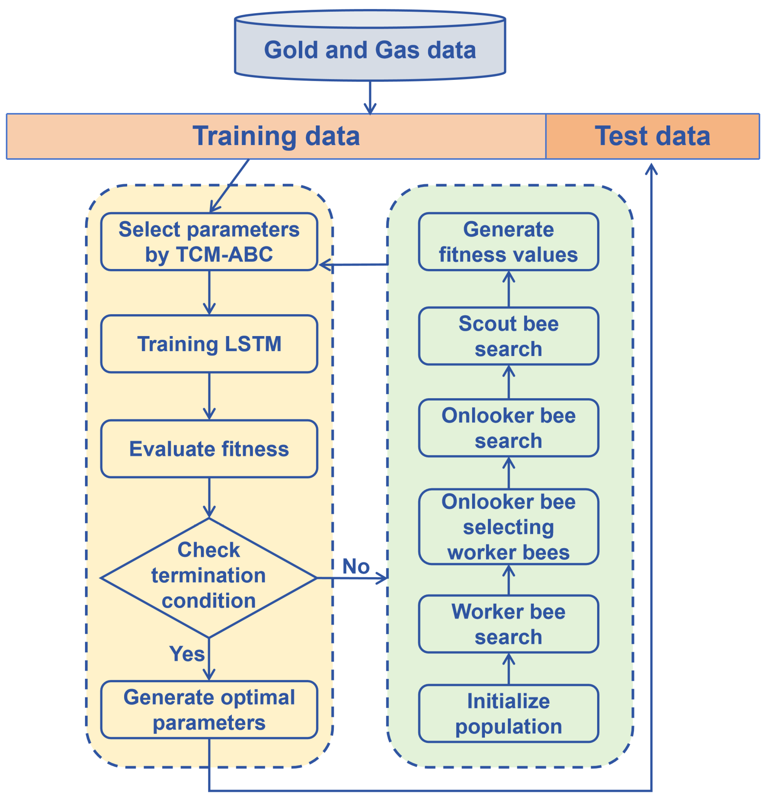Figure 3 displays the TCM-ABC-LSTM model’s concrete flowchart.

Figure 3. The flow chart of TCM-ABC-LSTM.

4. Experiment and Discussion

Gold and natural gas stand as pivotal commodities that command significant attention within the global futures market landscape. Often regarded as barometers of the world economy, fluctuations in the prices of gold and natural gas are closely scrutinized by investors and analysts alike. Changes in monetary policy, geopolitical threats, and inflation predictions are typically reflected in the direction of gold prices. Weather variations, geopolitical events, and supply–demand relationships all have an impact on natural gas prices. Recognizing the importance of comprehending market trends and making informed investment decisions, investors and stakeholders seek predictive models that can effectively anticipate price movements in these key commodities. To this end, our study opted to evaluate the predictive performance of the TCM-ABC-LSTM algorithm by focusing on futures prices for gold and natural gas commodities. By conducting a series of rigorous back-testing experiments on the next-day closing price indices of gold and natural gas futures, we aimed to elucidate the algorithm’s efficacy in forecasting commodity prices within the futures market domain. Table 1 provides a comprehensive overview of the hardware and software configurations utilized in our experimental setup, ensuring transparency and reproducibility in our methodology.

Table 1. The main hardware and software configurations.

Hardware/Software	Configuration
CPU	Kaggle CPU
GPU	NVIDIA Tesla P100
DISK	Max 73.1 GB
RAM	Max 29 GB
GPU memory	Max 16 GB
Python version	Python 3.7
Pytorch version	Pytorch 1.7.0

4.1. Data Description and Preprocessing

The opening, closing, highest, and lowest trade prices for natural gas from 4 April 1990–26 October 2023, and for gold from 2 January 1990–26 October 2023, are among the data analyzed in this study. Investing Financial Information provides the data instance for each index. Renowned as one of the premier financial websites globally, Investing Financial Information offers real-time updates and comprehensive market data on a diverse array of financial instruments, including stocks, funds, foreign currencies, futures, bonds, and digital currencies. One can download all of the experiment’s data at https://www.investing.com/commodities/real-time-futures, accessed on 11 June 2024. To facilitate effective model training and evaluation, the closing price data were partitioned into training and test sets. Specifically, the training set comprises the initial 80% of the data, employed to train the LSTM model parameters. Then, the remaining 20% of the data are reserved as a test set, serving as a robust validation mechanism for assessing the performance and accuracy of the proposed predictive model. It is worth noting that, in order to reduce the volatility of the dataset and enhance the predictive performance and stability of the proposed model, we normalize the raw data (both training and test sets) using Equation (16). This normalization process ensures that the raw data, both in the training and test sets, are standardized to a common scale, thereby facilitating more robust and reliable model training and evaluation, where $x_{min}$ and $x_{max}$ are the minimum and maximum values of the original sequence, respectively.

$$x_{i\left(norm\right)}=\frac{x_i-x_{min}}{x_{max}-x_{min}}$$

(16)

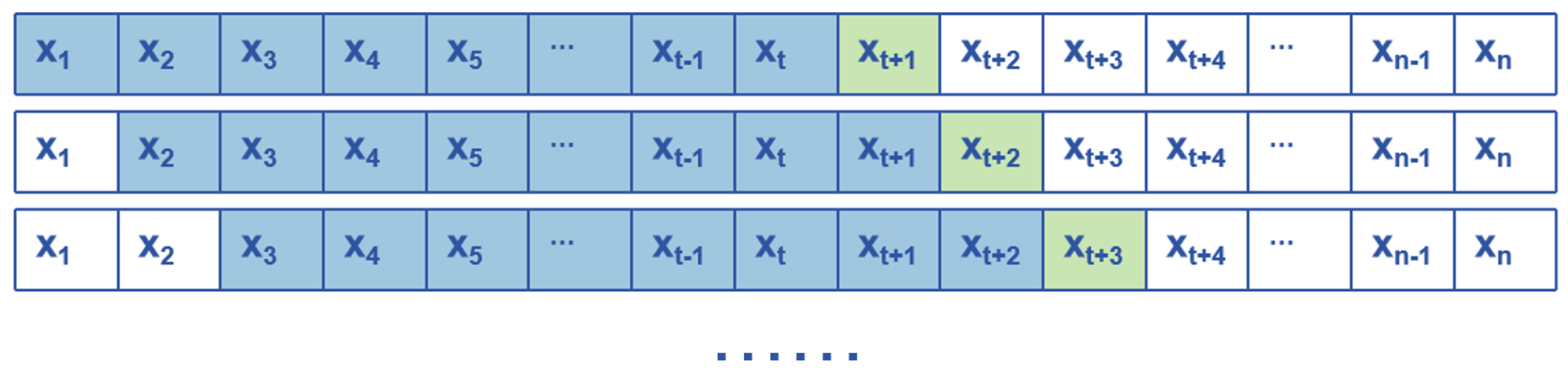
To facilitate this predictive process, we adopt the moving window method, a widely employed technique for feature extraction from observed time series data. The closing prices of the previous t trading days are used in each prediction to forecast the closing price of the following trading day t + 1. This method systematically constructs features and labels by sliding a window over the time series data, as depicted in Figure 4.

Figure 4. Moving window method.

4.2. Model Parameter Settings

We carried out a great deal of testing on the training set, and the pertinent parameters of the improved artificial bee colony algorithm were established as follows in light of many tests and related studies [40,41,42]: 50 honey sources, 500 iterations, 25 worker bees, and 15 onlooker bees. The number of LSTM’s hidden layer cells is given in [30, 200], the number of hidden layers is given in [1, 8], the time step is given in [20, 80], the batch size is given in [30, 80], and the epoch is given in [10, 500].

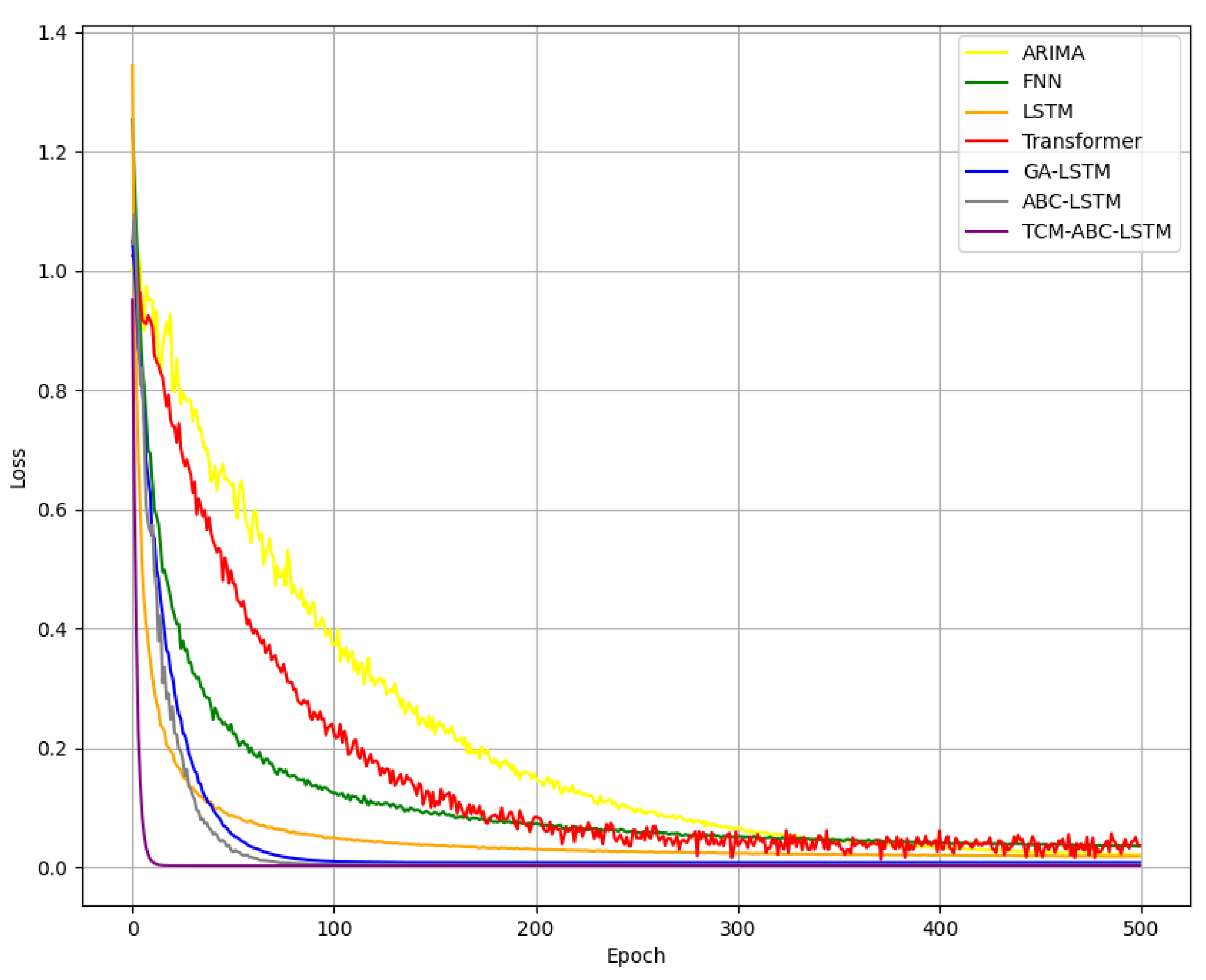
We use the root mean square error to evaluate the prediction accuracy. Taking the prediction of gold prices as an example, each algorithm’s loss function over time is displayed in Figure 5. The graph shows that our suggested algorithm has the fastest convergence speed and can reach the final result within approximately 10 iterations; second, the ABC-LSTM model can reach the final result after about 50 iterations, showing that the effect of our proposed swarm initialization operator on the speed of model training is effectual; and, finally, the Transformer model has the worst prediction performance, suggesting that it has limitations in capturing the intricate volatility patterns inherent in commodities traded on futures markets.

Figure 5. RMSE changes over time.

4.3. Evaluating Indicator

In this study, the model performance is evaluated by prediction accuracy, and we compare the predicted values to the real data in the test set and calculate the prediction error. The three prediction error evaluation metrics used in this study are as follows:

Mean Absolute Error (MAE):

$$MAE={\displaystyle \frac{1}{n}}\sum _{i=1}^n|p-\widehat{p}|$$

(17)

Mean Square Error (MSE):

$$MSE={\displaystyle \frac{1}{n}}\sum _{i=1}^n{(p-\widehat{p})}^2$$

(18)

Root Mean Square Error (RMSE):

$$RMSE=\sqrt{{\displaystyle \frac{1}{n}}\sum _{i=1}^n{(p-\widehat{p})}^2}$$

(19)

where p is the true value, $\widehat{p}$ is the predicted value, and n is the sample size. MAE is the mean absolute deviation between the predicted value and the true value, which ignores the direction of the error and focuses only on the magnitude of the error [43]. MSE is a common measure of time series forecasting performance. Similar to MAE, it also measures the absolute error in the forecast, which is squared, making MSE more sensitive to outliers but also more expressive of the distribution of the error [44]. RMSE is identical to the raw data in terms of magnitude and is therefore easier to visualize and understand. Similar to MSE, RMSE gives higher weight to large errors [45]. This study uses RMSE as the loss function for model training.

4.4. Results and Discussion

The empirical results of this study confirm the utility and effectiveness of the TCM-ABC-LSTM model. The same dataset is used to evaluate the prediction performance of the designed models relative to traditional neural networks and various meta-heuristic trainers, including ARIMA, LSTM, and GA-LSTM. Many researchers have demonstrated the high accuracy of the compared models before and used these models to improve many problems. Moreover, these models are among the most widely used and effective techniques in the field of prediction [29,46,47,48,49]. The performance and precision of our proposed model are evaluated in comparison to other prediction models, employing well-established metrics such as MAE, MSE, and RMSE. Among the diverse array of models compared in this study, our proposed model stands out, gaining the lowest mean absolute error, mean square error, and root mean square error, as shown in Table 2 and Table 3, bold indicates the best result for each indicator. Slight differences in these evaluation indicators have a big influence on forecast accuracy because of data standardization. To provide a comprehensive insight into the performance gains facilitated by our proposed model, using the MAE prediction results as an example, Table 4 elucidates the marked enhancements in prediction accuracy following inverse normalization. From the table, it can be seen that our model has a significantly improved prediction accuracy, with improvements ranging from 26.79% to 82.16% compared to other models. This indicates that the data volatility has been well captured in the fitted model, thereby affirming its robustness and efficacy as a futures prediction model.

Table 2. Performance comparison of gold price prediction models.

	MAE	MSE	RMSE
ARIMA	0.01188	$3.0\times {10}^{-4}$	0.0174
FNN	0.01902	$4.0\times {10}^{-4}$	0.0216
LSTM	0.00906	$1.2\times {10}^{-4}$	0.0110
Transformer	0.03253	$4.2\times {10}^{-3}$	0.6531
GA-LSTM	0.00755	$9.2\times {10}^{-5}$	0.0095
TCM-ABC-LSTM	0.00619	$\mathbf{6.7}\mathbf{\times }{\mathbf{10}}^{\mathbf{-}\mathbf{5}}$	0.0077

Table 3. Performance comparison of natural gas price prediction models.

	MAE	MSE	RMSE
ARIMA	0.01148	$2.2\times {10}^{-4}$	0.0149
FNN	0.00621	$1.1\times {10}^{-4}$	0.0109
LSTM	0.00630	$1.2\times {10}^{-4}$	0.0110
Transformer	0.02451	$1.3\times {10}^{-3}$	0.0368
GA-LSTM	0.00620	$7.8\times {10}^{-5}$	0.0088
TCM-ABC-LSTM	0.00250	$\mathbf{1.2}\mathbf{\times }{\mathbf{10}}^{\mathbf{-}\mathbf{5}}$	0.0035

Table 4. Model MAE performance improvement.

	ARIMA	FNN	LSTM	Transformer	GA-LSTM
MAE (decline)	57.18%	81.24%	56.59%	82.16%	26.79%

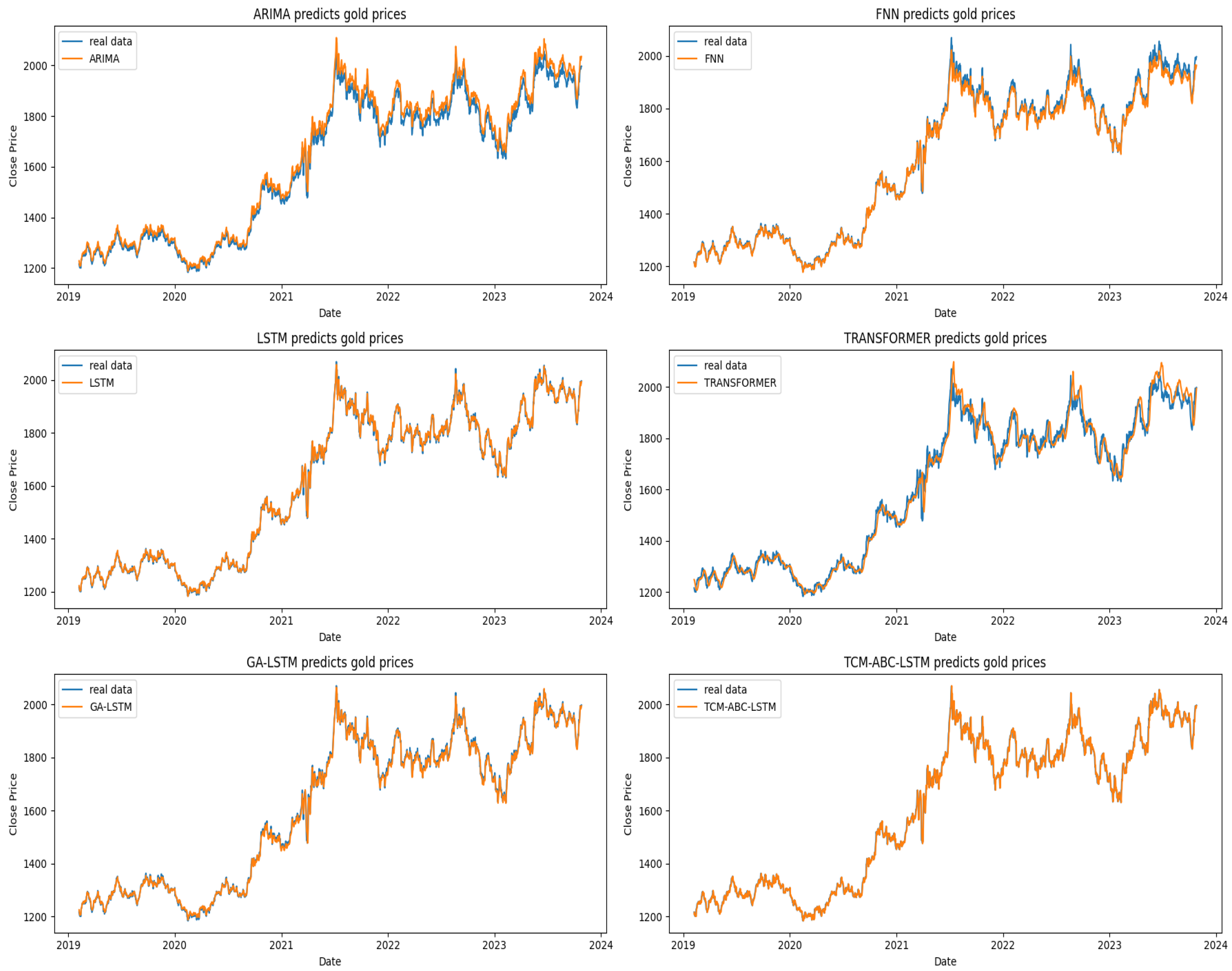
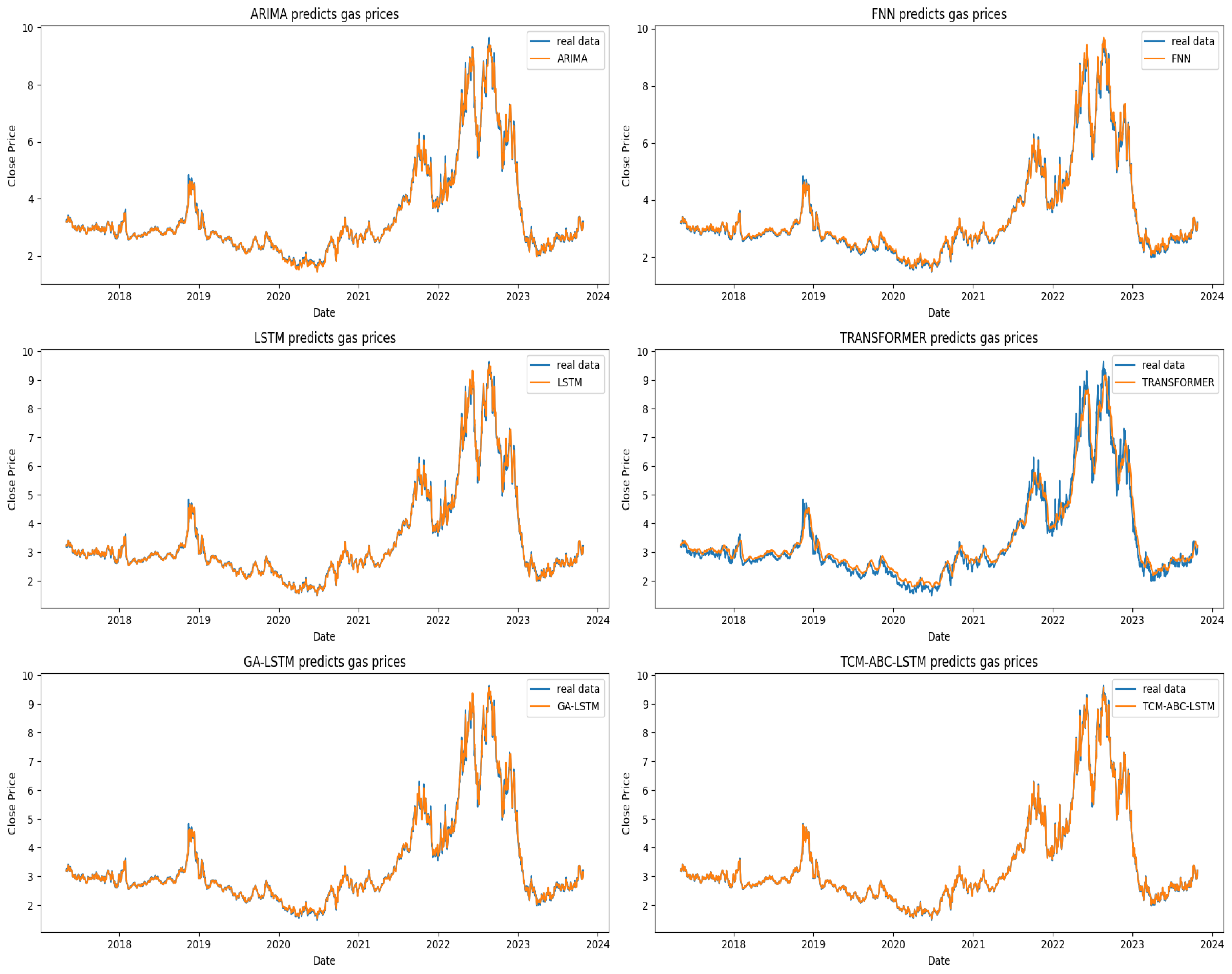
Figure 6 and Figure 7 illustrate how well the ARIMA, FNN, LSTM, Transformer, GA-LSTM, and TCM-ABC-LSTM models predict the prices of gold and natural gas, respectively. It is evident from the graph that the TCM-ABC-LSTM-predicted futures commodity prices closely match the actual data.

Figure 6. Prediction results of gold prices for various models.

Figure 7. Prediction results of natural gas prices for various models.

5. Conclusions

In this paper, we present a new model for predicting price fluctuations of futures commodities using an improved meta-heuristic algorithm TCM-ABC to train LSTM neural networks and apply it to predict the daily closing prices of gold and natural gas, comparing the obtained prediction results with those of classical neural networks and other meta-heuristic trainers such as ARIMA, Transformer, GA- LSTM, etc. The results show that the TCM-ABC-LSTM model outperforms the other models. The evaluation metrics reveal that the TCM-ABC-LSTM network model achieved the lowest MAE, MSE, and RMSE errors of $6.19\times {10}^{-3}$, $6.7\times {10}^{-5}$, and $7.7\times {10}^{-3}$, respectively. So far, the TCM-ABC-LSTM model is considered as a promising technique for high-precision commodity price prediction. We will explore more theoretical results in the future and expect that, in practice, investors can obtain higher excess returns through predictions of TCM-ABC-LSTM.

The gold and natural gas data used in this study are classical data from futures markets, and our proposed model performs very well on these datasets; we believe that the superior performance of TCM-ABC-LSTM is mainly attributed to the innovative improvement of the artificial bee colony algorithm and its application to LSTM networks. Compared with the traditional LSTM model, the proposed TCM-ABC-LSTM model has better generalization ability because it can adaptively find the optimal hyperparameters. However, there are some limitations in this study, such as that this paper only predicts the closing price of the commodity on the following day alone, but, in fact, the longer the prediction time, the more insight into the future trend of the commodity for further analysis. These will be discussed in our future research. In the future, additional research will be carried out on the following points:

• Extending the application of the TCM-ABC-LSTM model to diverse time series prediction tasks encompassing domains such as electricity consumption, wind power generation, and stock market dynamics.
• Exploring alternative optimization algorithms to serve as hyperparameter selectors for LSTM models in the quest for better hybrid models.
• Applying long-term sequence prediction using the proposed model.