
A Deep Learning-Based Ultrasonic Diffraction Data Analysis Method for Accurate Automatic Crack Sizing

 ,
, 
Abstract
Featured Application
Abstract
1. Introduction
2. Ultrasonic Diffraction Theory Background
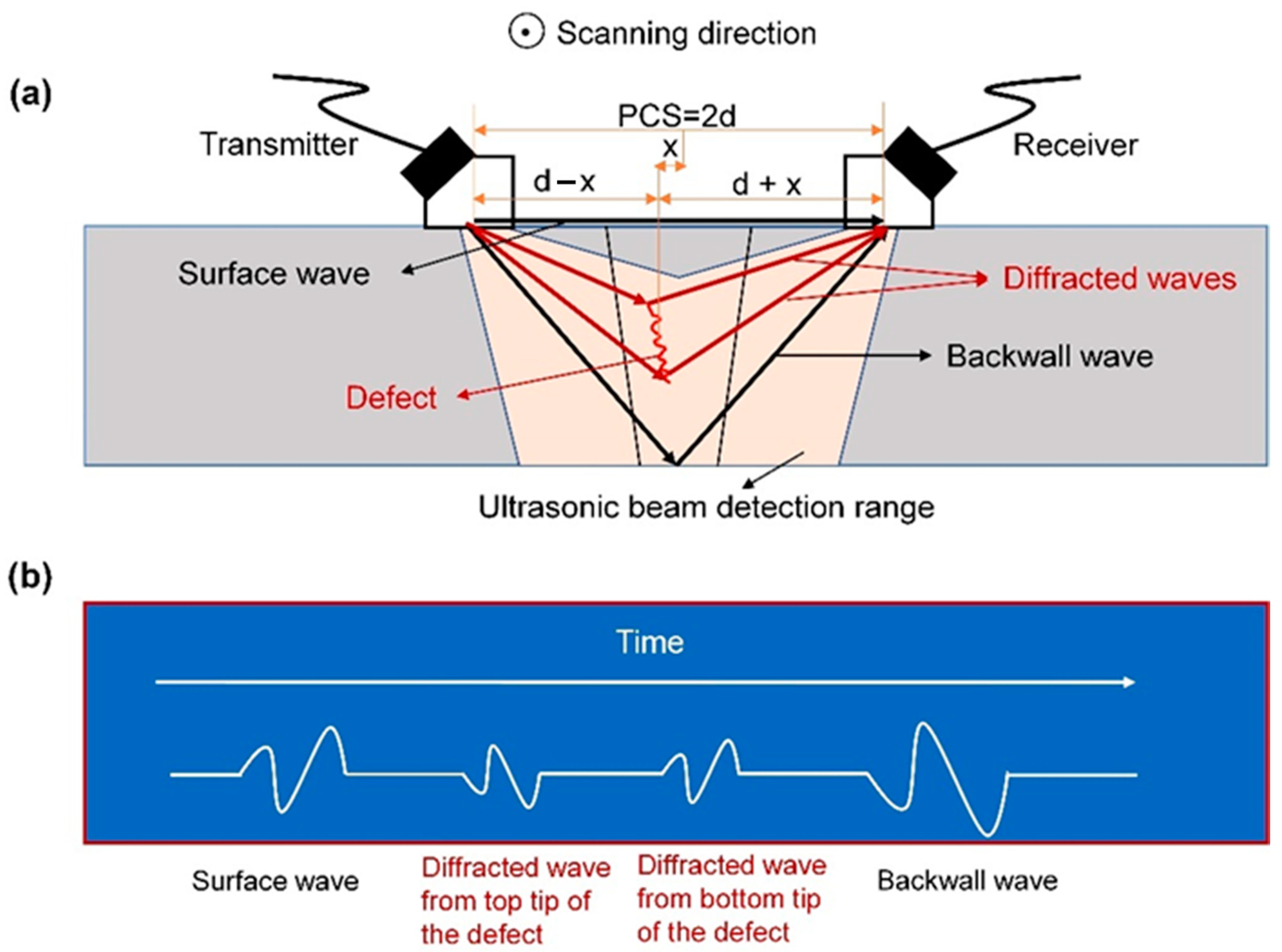
2.1. Flight Diffraction Model
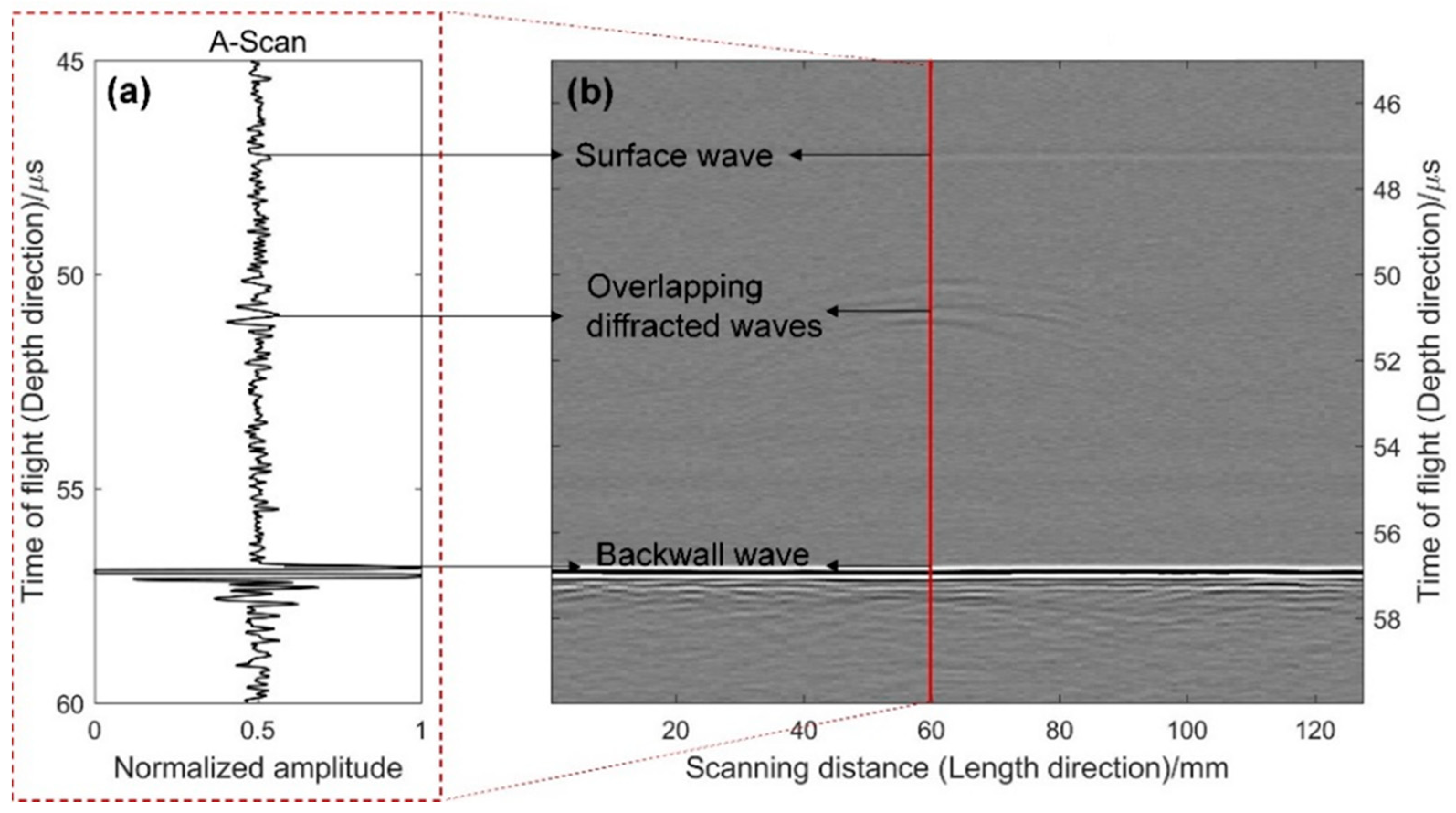
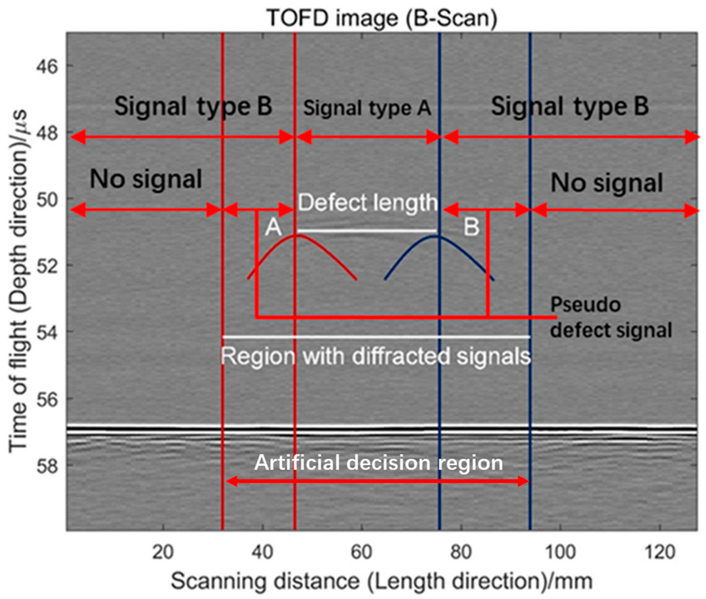
2.2. Image Generation
3. Deep Learning-Based Crack Sizing Method
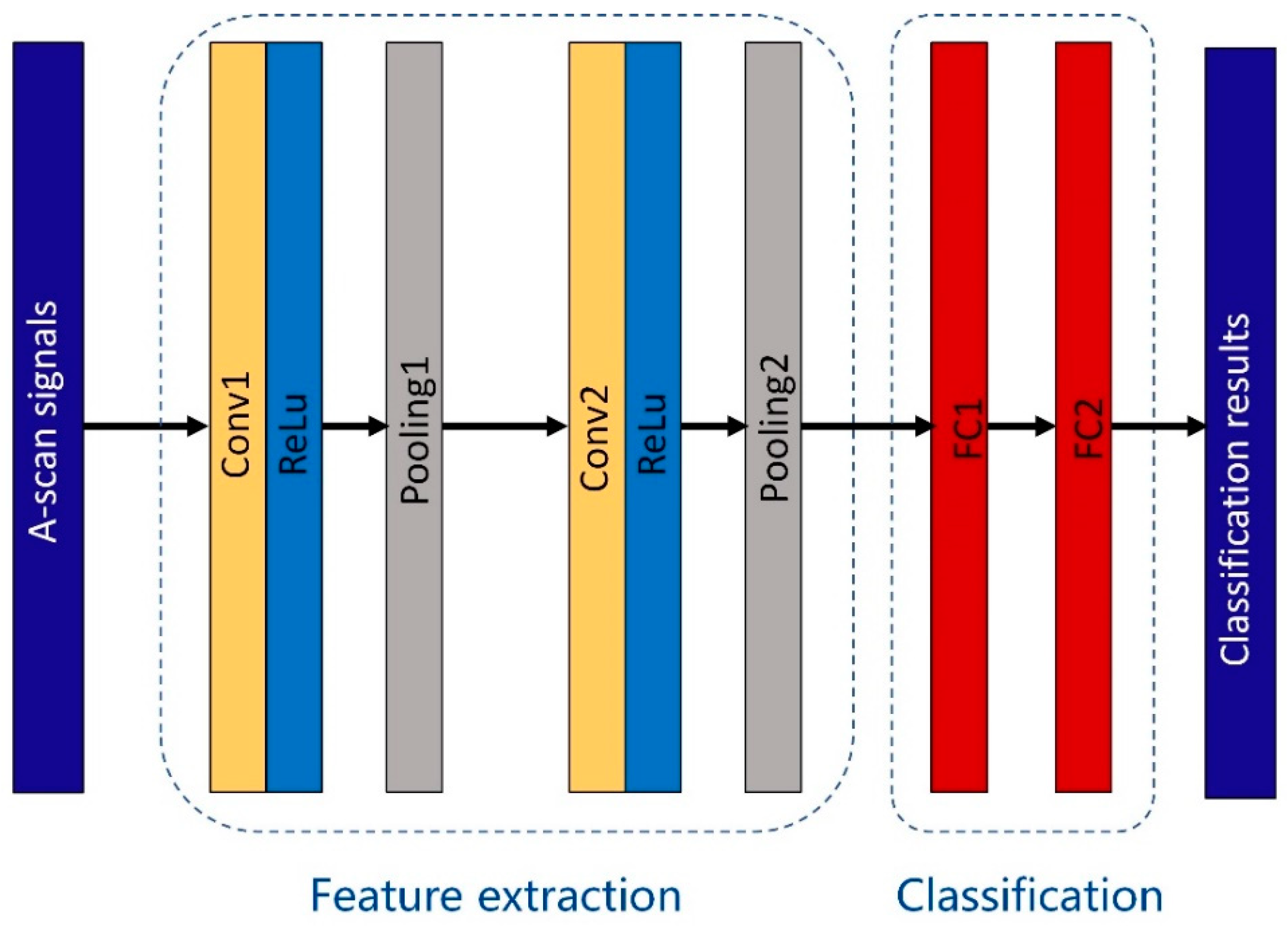
3.1. Length Measurement Architecture
3.2. Height Measurement Architecture
4. Data Acquisition
4.1. Experimental Setup
4.2. Ultrasonic Dataset
5. Results and Discussion
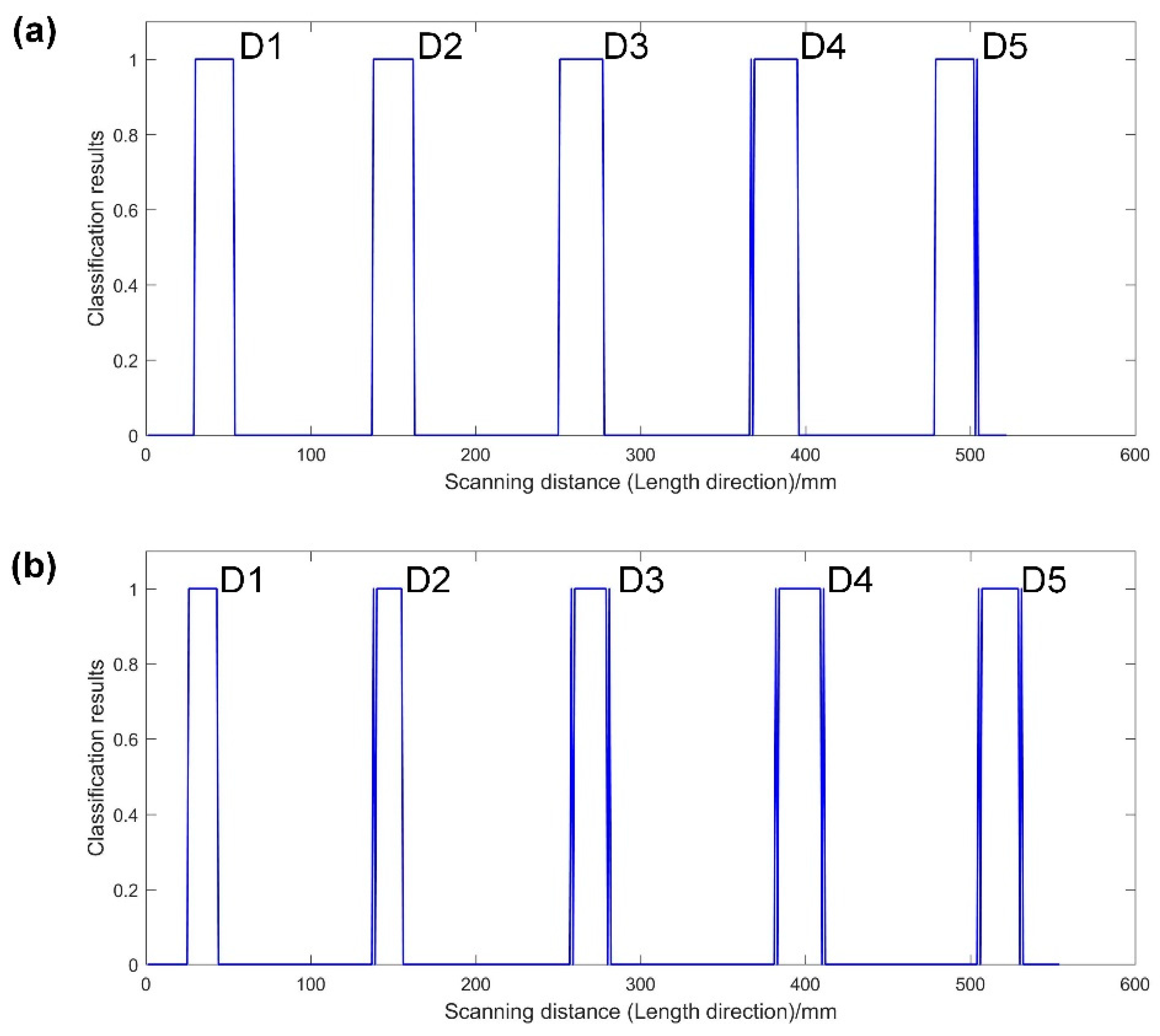
5.1. Length Measurement Results and Discussion
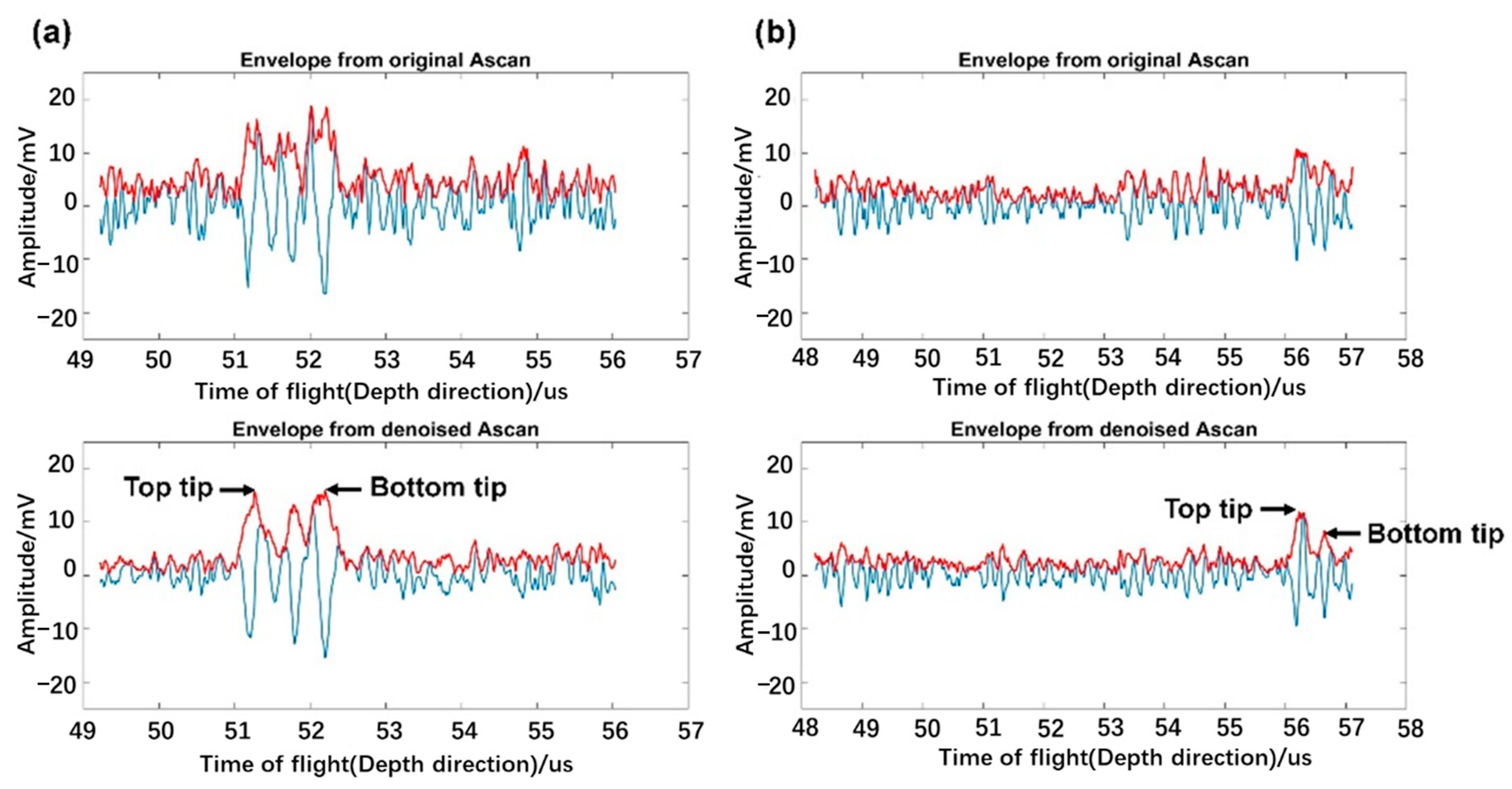
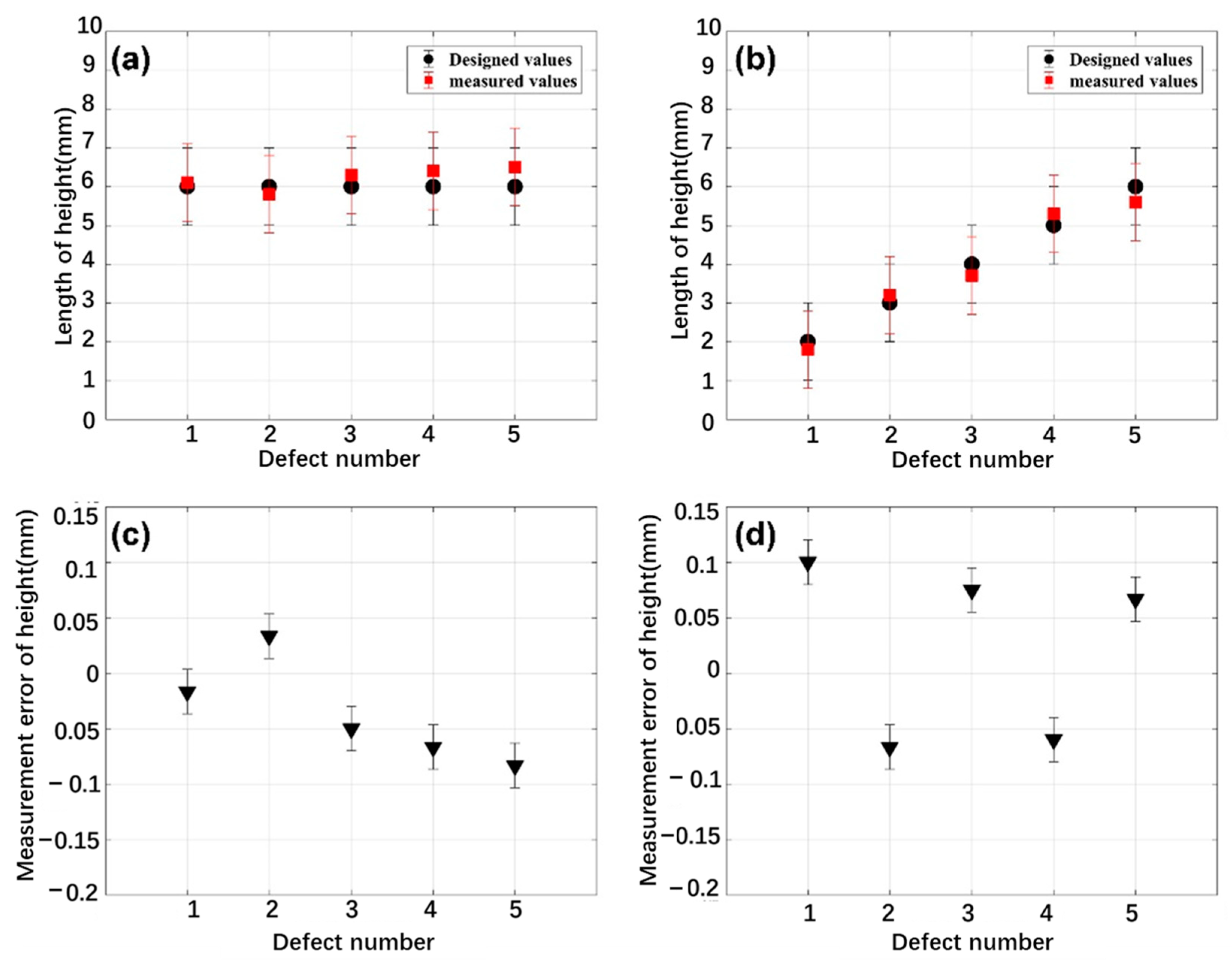
5.2. Height Measurement Results and Discussion
6. Conclusions
Author Contributions
Funding
Institutional Review Board Statement
Informed Consent Statement
Data Availability Statement
Acknowledgments
Conflicts of Interest
References
- Silk, M.G. Interpretation of TOFD data in the light of ASME XI and similar rules. Brit. J. Non Destr. Test. 1989, 31, 242–251. [Google Scholar]
- Silk, M.G.; Lidington, B.H. Defect sizing using an ultrasonic time delay approach. Brit. J. Non Destr. Test. 1975, 17, 33–36. [Google Scholar]
- Jin, S.; Wang, X.; Wang, Z.; Luo, Z. Defect detection of spherical heads by time-of-flight diffraction. Appl. Acoust. 2024, 216, 109787. [Google Scholar] [CrossRef]
- Silk, M.G.; Lidington, B.H. The potential of scattered or diffracted ultrasound in the determination of crack depth. Non Destr. Test. 1975, 8, 146–151. [Google Scholar] [CrossRef]
- Han, Q.; Wang, P.; Zheng, H. Modified ultrasonic time-of-flight diffraction testing with Barker code excitation for sizing inclined crack. Appl. Acoust. 2018, 140, 153–159. [Google Scholar] [CrossRef]
- Carvalho, A.; Rebello, J.; Souza, M.; Sagrilo, L.; Soares, S. Reliability of non-destructive test techniques in the inspection of pipelines used in the oil industry. Int. J. Press. Vessel. Pip. 2008, 85, 745–751. [Google Scholar] [CrossRef]
- Bolland, P.; Voon, L.L.; Gremillet, B.; Pillet, L.; Diou, A.; Gorria, P. The application of Hough transform on ultrasonic images for the detection and characterization of defects in non-destructive inspection. In Proceedings of the Third International Conference on Signal Processing (ICSP’96), Beijing, China, 18 October 1996; Volume 391, pp. 393–396. [Google Scholar]
- Merazi-Meksen, T.; Boudraa, M.; Boudraa, B. Mathematical morphology for TOFD image analysis and automatic crack detection. Ultrasonics 2014, 54, 1642–1648. [Google Scholar] [CrossRef] [PubMed]
- Bolland, P.; Voon, L.L.; Gorria, P.; Gremillet, B.; Pillet, L. Gradient-based Hough transform for the detection and characterization of defects during non-destructive inspection. In Proceedings of the IEEE/ASME International Conference on Advanced Intelligent Mechatronics, Tokyo, Japan, 20 June 1997; p. 33. [Google Scholar]
- Maalmi, K.; Benslimane, R.; Voon, L.L.Y.; Eric, F. Towards automatic analysis of ultrasonic time-of-flight diffraction data using genetic-based Inverse Hough Transform. Insight 2009, 51, 184–191. [Google Scholar] [CrossRef]
- Petcher, P.A.; Dixon, S. Parabola detection using matched filtering for ultrasound B-scans. Ultrasonics 2012, 52, 138–144. [Google Scholar] [CrossRef]
- Hirata, S.; Kurosawa, M.K. Ultrasonic distance and velocity measurement using a pair of LPM signals for cross-correlation method: Improvement of Doppler-shift compensation and examination of Doppler velocity estimation. Ultrasonics 2012, 52, 873–879. [Google Scholar] [CrossRef]
- Queiros, R.; Girao, P.S.; Serra, A.C. Cross-Correlation and Sine-Fitting Techniques for High Resolution Ultrasonic Ranging. IEEE Trans. Instrum. Meas. 2006, 59, 552–556. [Google Scholar]
- Demirli, R.; Saniie, J. Model-based estimation of ultrasonic echoes. Part I: Analysis and algorithms. IEEE Trans. Ultrason Ferroelectr. Freq. Control. 2001, 48, 787–802. [Google Scholar] [CrossRef]
- Demirli, R.; Saniie, J. Model-based estimation of ultrasonic echoes. Part II: Nondestructive evaluation applications. IEEE Trans. Ultrason Ferroelectr. Freq. Control. 2001, 48, 803–811. [Google Scholar] [CrossRef] [PubMed]
- Ruiz-Reyes, N.; Vera-Candeas, P.; Curpián-Alonso, J.; Mata-Campos, R.; Cuevas-Martínez, J.C. New matching pursuit-based algorithm for SNR improvement in ultrasonic NDT. Non Destr. Test. E Int. 2005, 38, 453–458. [Google Scholar] [CrossRef]
- Yacef, N.; Bouden, T.; Grimes, M. Accurate ultrasonic measurement technique for crack sizing using envelope detection and differential evolution. Non Destr. Test. E Int. 2019, 102, 161–168. [Google Scholar] [CrossRef]
- Zhi, Z.; Jiang, H.; Yang, D.; Gao, J.; Wang, Q.; Wang, X.; Wang, J.; Wu, Y. An end-to-end welding defect detection approach based on titanium alloy time-of-flight diffraction images. J. Intell. Manuf. 2023, 34, 1895–1909. [Google Scholar] [CrossRef]
- Medak, D.; Posilović, L.; Subašić, M.; Budimir, M.; Lončarić, S. DefectDet: A deep learning architecture for detection of defects with extreme aspect ratios in ultrasonic images. Neurocomputing 2022, 473, 107–115. [Google Scholar] [CrossRef]
- Felice, M.V.; Fan, Z. Sizing of flaws using ultrasonic bulk wave testing: A review. Ultrasonics 2018, 88, 26–42. [Google Scholar] [CrossRef]
- Browne, B. Time of flight diffraction its limitations–actual & perceived. E-J. Non. Destr. Test. 1997, 2. Available online: https://www.ndt.net/?id=179 (accessed on 6 April 2024).
- Hu, Q.; Wei, X.; Guo, H.; Xu, H.; Li, C.; He, W.; Pei, B. Study on intelligent and visualization method of ultrasonic testing of composite materials based on deep learning. Appl. Acoust. 2023, 207, 109363. [Google Scholar] [CrossRef]
- Masnata, A.; Sunseri, M. Neural network classification of flaws detected by ultrasonic means. Non Destr. Test. E Int. 1996, 29, 87–93. [Google Scholar] [CrossRef]
- Margrave, F.W.; Rigas, K.; Bradley, D.A.; Barrowcliffe, P. The use of neural networks in ultrasonic flaw detection. Measurement 1999, 25, 143–154. [Google Scholar] [CrossRef]
- Drai, R.; Khelil, M.; Benchaala, A. Time frequency and wavelet transform applied to selected problems in ultrasonics NDE. Non Destr. Test. E Int. 2002, 35, 567–572. [Google Scholar] [CrossRef]
- Filho, E.F.S.; Silva, M.M.; Farias, P.C.M.A.; Albuquerque, M.C.S.; Silva, I.C.; Farias, C.T.T. Flexible decision support system for ultrasound evaluation of fiber–metal aminates implemented in a DSP. Non Destr. Test. E Int. 2016, 79, 38–45. [Google Scholar]
- Munir, N.; Kim, H.-J.; Song, S.-J.; Kang, S.-S. Investigation of deep neural network with drop out for ultrasonic flaw classification in weldments. J. Mech. Sci. Technol. 2018, 32, 3073–3080. [Google Scholar] [CrossRef]
- Munir, N.; Kim, H.-J.; Park, J.; Song, S.-J.; Kang, S. Convolutional neural network for ultrasonic weldment flaw classification in noisy conditions. Ultrasonics 2019, 94, 74–81. [Google Scholar] [CrossRef] [PubMed]
- Meng, M.; Chua, Y.J.; Wouterson, E.; Ong, C.P.K. Ultrasonic signal classification and imaging system for composite materials via deep convolutional neural networks. Neurocomputing 2017, 257, 128–135. [Google Scholar] [CrossRef]
- Lecun, Y.; Bottou, L.; Bengio, Y.; Haffner, P. Gradient-based learning applied to document recognition. Proc. IEEE 1998, 86, 2278–2324. [Google Scholar] [CrossRef]
- Lecun, Y.; Bengio, Y.; Hinton, G. Deep learning. Nature 2015, 521, 436–444. [Google Scholar] [CrossRef]
- Schmidhuber, J. Deep learning in neural networks: An overview. Neural Netw. 2015, 61, 85–117. [Google Scholar] [CrossRef]
- Xu, W.; Li, X.; Zhang, J.; Xue, Z.; Cao, J. Ultrasonic signal enhancement for coarse grain materials by machine learning analysis. Ultrasonics 2021, 117, 106550. [Google Scholar] [CrossRef] [PubMed]
- Xu, W.; Zhang, J.; Li, X.; Yuan, S.; Ma, G.; Xue, Z.; Jing, X.; Cao, J. Intelligent denoise laser ultrasonic imaging for inspection of selective laser melting components with rough surface. Non Destr. Test. E Int. 2022, 125, 102548. [Google Scholar] [CrossRef]
- Rashid, T. Make Your Own Neural Network; CreateSpace Independent Publishing Platform: Scotts Valley, CA, USA, 2016. [Google Scholar]


| Layer Type | Number of Input Channel | Number of Output Channel | Kernel Size/ Stride | Features Maps | Padding |
|---|---|---|---|---|---|
| Conv 1 | 1 | 16 | 8 × 1/2 | 16 × 445 × 1 | Same |
| Pooling 1 | - | - | 2 × 1/2 | 16 × 223 × 1 | Same |
| Conv 2 | 16 | 32 | 4 × 1/2 | 32 × 111 × 1 | Same |
| Pooling 2 | - | - | 2 × 1/2 | 32 × 56 × 1 | Same |
| FC dropout | - | - | 0.25 | - | - |
| FC | - | - | 200 | - | - |
| Output | - | - | 2 | - | - |
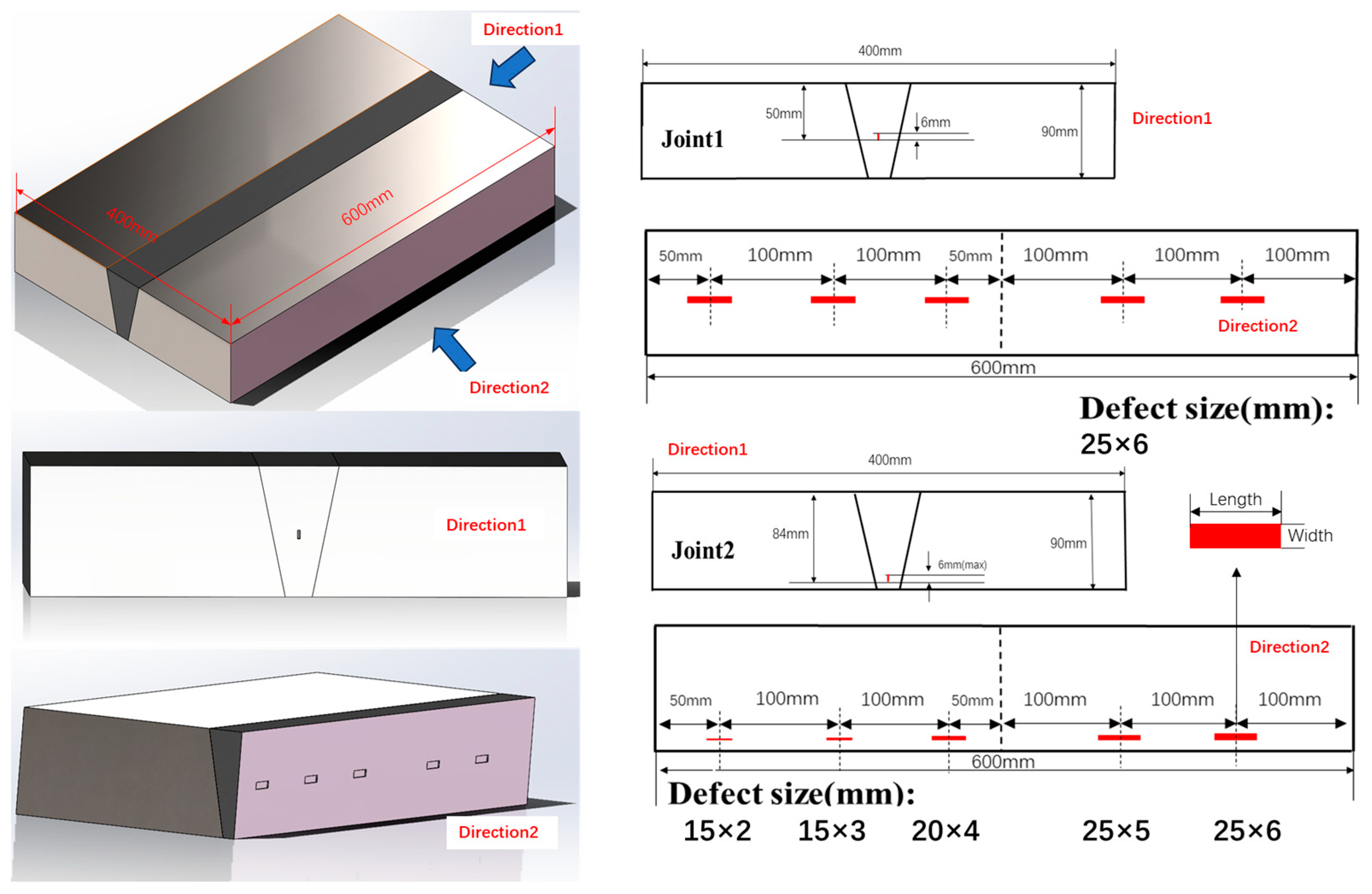
| Welded Joint Number | Defect Number | Length | Height | Depth |
|---|---|---|---|---|
| Joint1 | D1 | 25 | 6 | 50 |
| D2 | 25 | 6 | 50 | |
| D3 | 25 | 6 | 50 | |
| D4 | 25 | 6 | 50 | |
| D5 | 25 | 6 | 50 | |
| Joint2 | D1 | 15 | 2 | 84 |
| D2 | 15 | 3 | 84 | |
| D3 | 20 | 4 | 84 | |
| D4 | 25 | 5 | 84 | |
| D5 | 25 | 6 | 84 |
| Welded Joint Number | Defect Number | Designed Value | Measured Value |
|---|---|---|---|
| Joint1 | D1 | 25 | 23 |
| D2 | 25 | 24 | |
| D3 | 25 | 26 | |
| D4 | 25 | 27 | |
| D5 | 25 | 24 | |
| Joint2 | D1 | 15 | 17 |
| D2 | 15 | 16 | |
| D3 | 20 | 21 | |
| D4 | 25 | 27 | |
| D5 | 25 | 24 |
| Welded Joint Number | Defect Number | Designed Value | Measured Value |
|---|---|---|---|
| Joint1 | D1 | 6 | 6.1 |
| D2 | 6 | 5.8 | |
| D3 | 6 | 6.3 | |
| D4 | 6 | 6.4 | |
| D5 | 6 | 6.5 | |
| Joint2 | D1 | 2 | 1.8 |
| D2 | 3 | 3.2 | |
| D3 | 4 | 3.7 | |
| D4 | 5 | 5.3 | |
| D5 | 6 | 5.6 |
Disclaimer/Publisher’s Note: The statements, opinions and data contained in all publications are solely those of the individual author(s) and contributor(s) and not of MDPI and/or the editor(s). MDPI and/or the editor(s) disclaim responsibility for any injury to people or property resulting from any ideas, methods, instructions or products referred to in the content. |
© 2024 by the authors. Licensee MDPI, Basel, Switzerland. This article is an open access article distributed under the terms and conditions of the Creative Commons Attribution (CC BY) license (https://creativecommons.org/licenses/by/4.0/).
Share and Cite
Fei, Q.; Cao, J.; Xu, W.; Jiang, L.; Zhang, J.; Ding, H.; Yan, J. A Deep Learning-Based Ultrasonic Diffraction Data Analysis Method for Accurate Automatic Crack Sizing. Appl. Sci. 2024, 14, 4619. https://doi.org/10.3390/app14114619
Fei Q, Cao J, Xu W, Jiang L, Zhang J, Ding H, Yan J. A Deep Learning-Based Ultrasonic Diffraction Data Analysis Method for Accurate Automatic Crack Sizing. Applied Sciences. 2024; 14(11):4619. https://doi.org/10.3390/app14114619
Chicago/Turabian StyleFei, Qinnan, Jiancheng Cao, Wanli Xu, Linzhao Jiang, Jun Zhang, Hui Ding, and Jingli Yan. 2024. "A Deep Learning-Based Ultrasonic Diffraction Data Analysis Method for Accurate Automatic Crack Sizing" Applied Sciences 14, no. 11: 4619. https://doi.org/10.3390/app14114619
APA StyleFei, Q., Cao, J., Xu, W., Jiang, L., Zhang, J., Ding, H., & Yan, J. (2024). A Deep Learning-Based Ultrasonic Diffraction Data Analysis Method for Accurate Automatic Crack Sizing. Applied Sciences, 14(11), 4619. https://doi.org/10.3390/app14114619