You are currently viewing a new version of our website. To view the old version click .
Applied Sciences
  • Article
  • Open Access

23 May 2024

Synergizing Transfer Learning and Multi-Agent Systems for Thermal Parametrization in Induction Traction Motors

,
and
1
School of Innovation, Design and Technology (IDT), Mälardalen University (MDU), 631 05 Eskilstuna, Sweden
2
Alstom, 721 36 Västerås, Sweden
*
Author to whom correspondence should be addressed.
This article belongs to the Special Issue Special Issue for the 64th International Conference of Scandinavian Simulation Society, SIMS 2023

Abstract

Maintaining optimal temperatures in the critical parts of an induction traction motor is crucial for railway propulsion systems. A reduced-order lumped-parameter thermal network (LPTN) model enables computably inexpensive, accurate temperature estimation; however, it requires empirically based parameter estimation exercises. The calibration process is typically performed in labs in a controlled experimental setting, which is associated with a lot of supervised human efforts. However, the exploration of machine learning (ML) techniques in varied domains has enabled the model parameterization in the drive system outside the laboratory settings. This paper presents an innovative use of a multi-agent reinforcement learning (MARL) approach for the parametrization of an LPTN model. First, a set of reinforcement learning agents are trained to estimate the optimized thermal parameters using the simulated data in several driving cycles (DCs). The selection of a reinforcement learning agent and the level of neurons in the RL model is made based on variability of the driving cycle data. Furthermore, transfer learning is performed on a new driving cycle data collected on the measurement setup. Statistical analysis and clustering techniques are proposed for the selection of an RL agent that has been pre-trained on the historical data. It is established that by synergizing within reinforcement learning techniques, it is possible to refine and adjust the RL learning models to effectively capture the complexities of thermal dynamics. The proposed MARL framework shows its capability to accurately reflect the motor’s thermal behavior under various driving conditions. The transfer learning usage in the proposed approach could yield significant improvement in the accuracy of temperature prediction in the new driving cycles data. This approach is proposed with the aim of developing more adaptive and efficient thermal management strategies for railway propulsion systems.

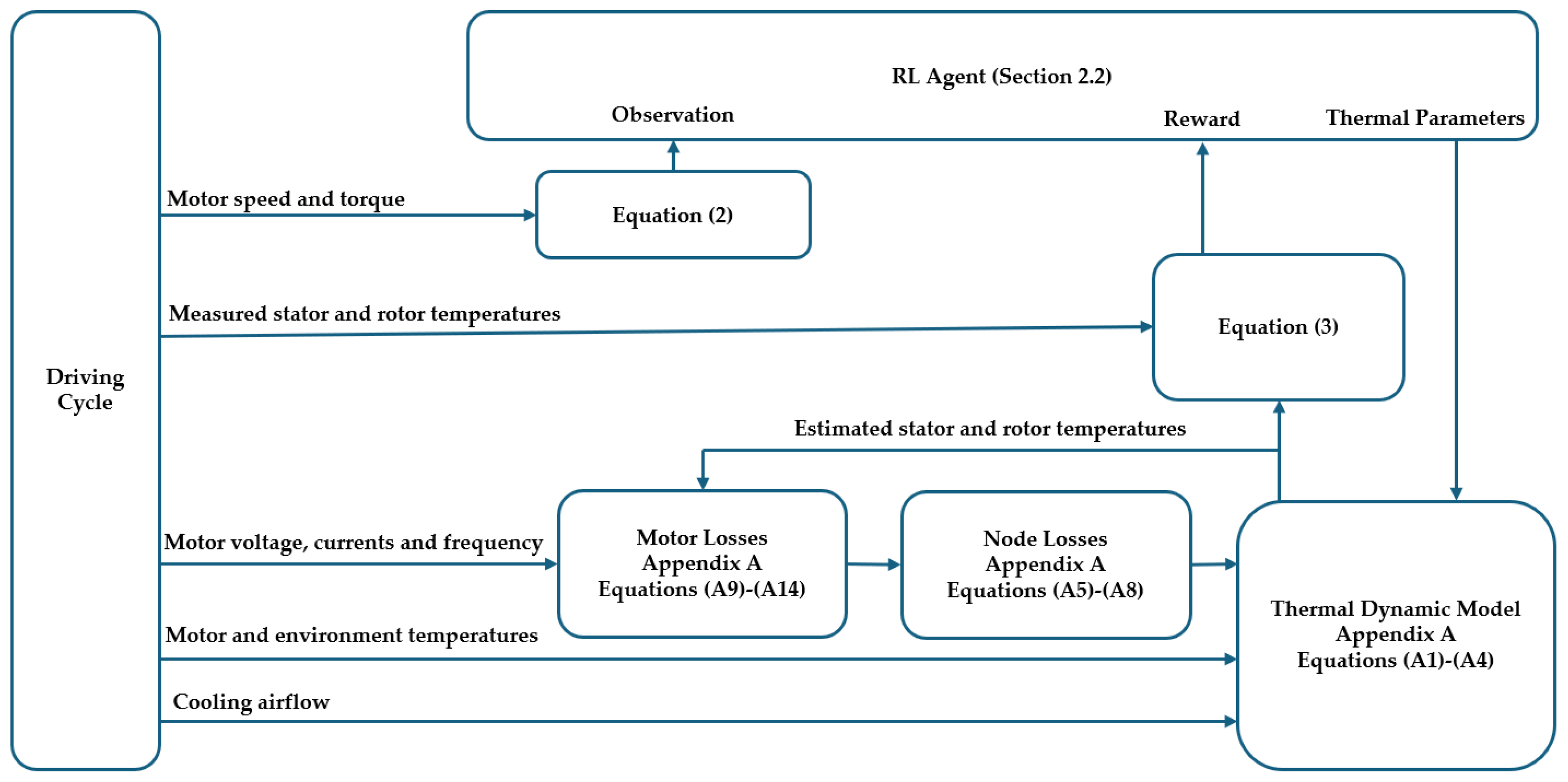
2. Multi-Agent Reinforcement Learning Framework and Transfer Learning Approach

The multi-agent reinforcement learning (MARL)-based framework takes the idea of making smart choices from single-agent RL and can handle complex problems that get harder and harder as they grow. MARL makes smart decisions by trying different actions and seeing what works best. Each RL agent learns from its environment and the other agents to improve the whole team’s results. This teamwork approach is efficient at solving complex problems that one agent alone could not handle, leading to smarter and more efficient solutions in real-world applications.
In synergizing the transfer learning approach, pre-trained reinforcement learning models are fine-tuned when applied to new similar driving cycles. In the proposed method, based on the source domain comprising several driving cycles on which the MARL models were initially trained, the model predicts the temperature in the target domain. The trained RL model includes important knowledge learned from the historical driving cycles’ dataset. Thus, the model can utilize this existing or learned knowledge to make predictions on a new driving cycle efficiently. Nonetheless, the reinforcement learning pre-trained model’s knowledge may not absolutely be aligned with the complexities of the new driving cycle data when the operation environment changes. Therefore, fine-tuning or change of a few parameters in the model must be performed to accurately predict the temperature. Thus, the pre-trained reinforcement learning models can be adjusted to optimize performance while taking advantage of the information acquired during pre-training.
Combining transfer learning with the MARL approach, the ability to handle the nonlinearity of the thermal model and parasitic influences from other drive system components in the training process could be enhanced, thus making it suitable for real-time implementation. In addition, by transfer learning, the agents adapt and make informed decisions which potentially improves the overall performance and efficiency of the thermal model. This synergy between transfer learning and the MARL framework has the potential to develop an adaptive and robust solution that works for real-world dynamic scenarios.

2.1. The Reinforcement Learning Framework

A data-driven, reinforcement-learning-based parametrization method was proposed in our previous work [35] to estimate the thermal parameters of the thermal model of an induction traction motor as depicted in Figure 1. The thermal model has been parametrized as detailed in Appendix A. The RL agent uses a weighted combination of motor speed and torque as observation, Equation (2), and a weighted sum of the absolute differences between the measured and estimated temperatures as a reward, Equation (3), to produce the thermal parameters that maximize the reward value. The next sections explain various types of RL agents and the training process.
O b s e r v a t i o n = ω 1 M S , ω 2 M T
R e w a r d = ω 3 ω 4 T s m T s e + ω 5 T r m T r e + ω 6
where M S ,   M T are motor speed and torque, respectively; T s m T s e is the absolute value of the difference between measured stator temperature ( T s m ) and estimated stator temperature ( T s e ); T r m T r e is the absolute value of the difference between measured rotor temperature ( T r m ) and estimated rotor temperature ( T r e ); and ω i ,   i = 1,2 , , 6 are positive weights.
Figure 1. The reinforcement learning framework (adopted from [35], see Appendix A).

2.2. RL Multiple Agents Composition

The proposed data-driven approach employs three distinct reinforcement learning agents, twin delayed deep deterministic policy gradient (TD3), soft actor-critic (SAC), and deep deterministic policy gradient (DDPG). These agents are used to predict temperature based on the simulated data in nine operational driving cycles and the measurement data for one driving cycle.

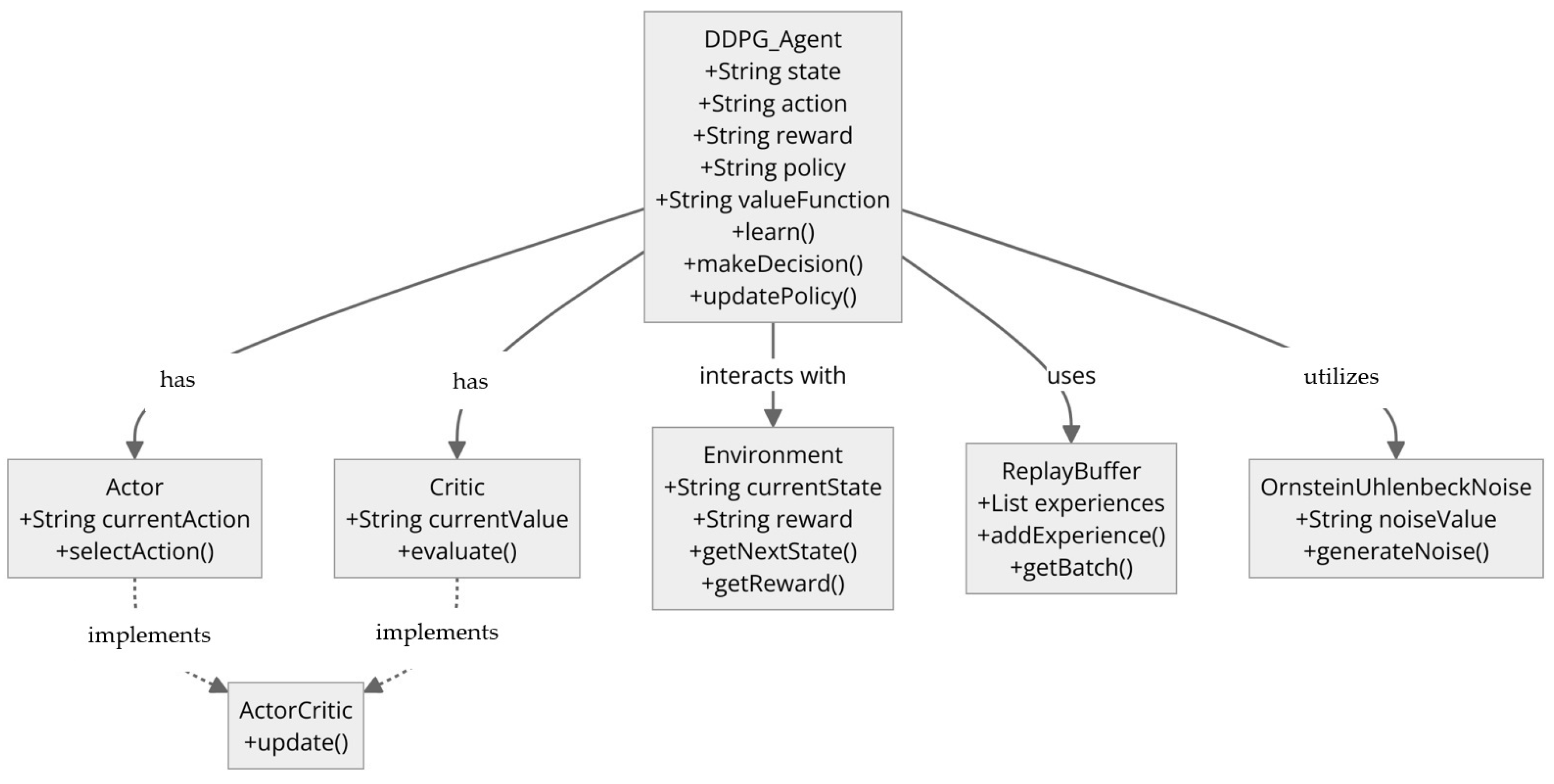
2.2.1. Twin-Delayed Deep Deterministic Policy Gradient (TD3) Structure

The TD3 strategy employs a single-actor network with two critic networks as shown in Figure 2. These networks are deep neural networks that use observations, actions, and rewards which are gathered from the Experience Replay Buffer. The Experience Replay Buffer stores past experiences to allow the learning algorithm to benefit from a wide range of scenarios. The TD3 algorithm ensures that the actor and critic models are effectively trained to predict and evaluate the output of actions taken in the actual environment.
Figure 2. The architecture of the TD3 agent.

2.2.2. Deep Deterministic Policy Gradient (DDPG) Agent Structure

The DDPG agent combines the benefits of both policy gradient and value-based approaches. This framework excels in managing high-dimensional, continuous action spaces, making it particularly suitable for complex control tasks. The DDPG framework consists of four key components as shown in Figure 3 such as an actor network that proposes actions. A critic network evaluates the actions’ potential reward and a target actor and critic network. These components use a replay buffer to store experiences and an update mechanism is used to combine target network parameters with the main networks.
Figure 3. The architecture of the DDPG agent.

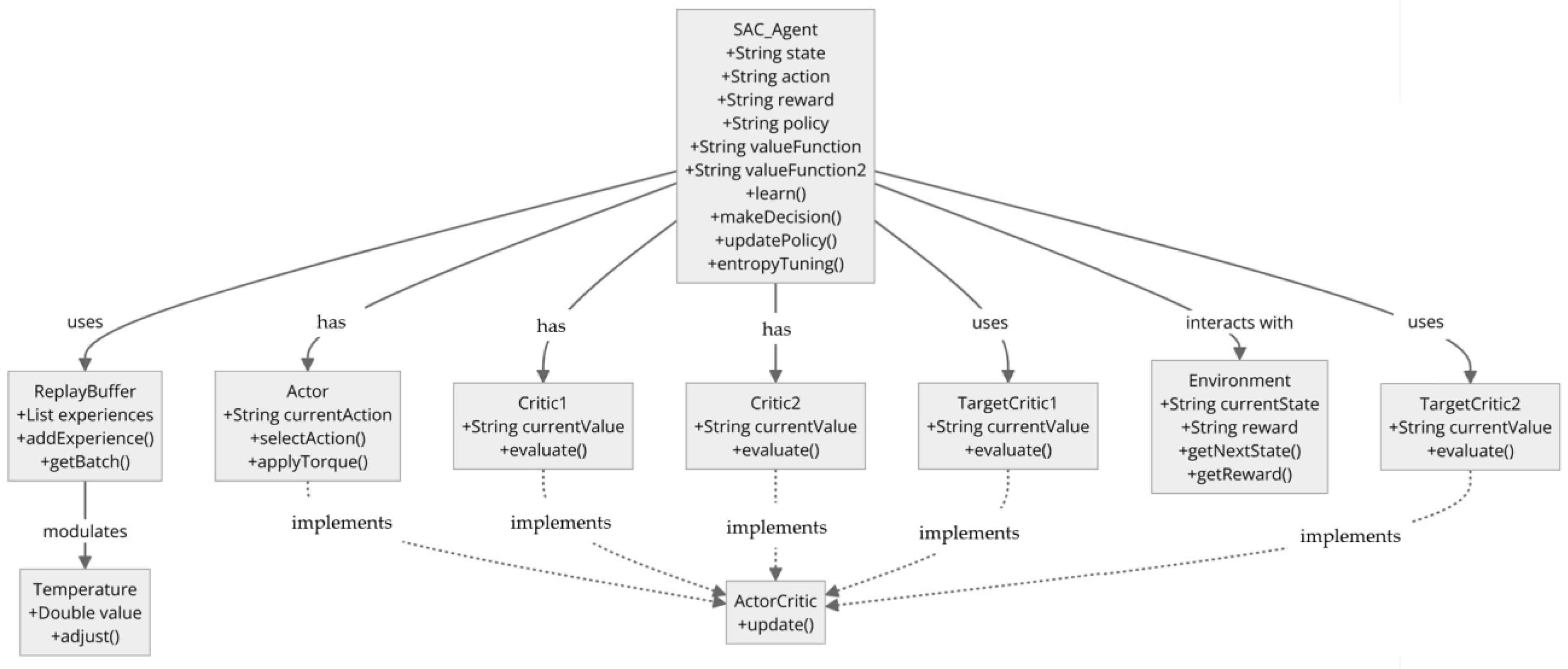
2.2.3. Soft Actor-Critic (SAC) Agent Structure

The SAC agent represents an advanced reinforcement learning strategy that emphasizes entropy in the policy for exploration. The SAC agent comprises a dual critic design to minimize the overestimation bias, as shown in Figure 4. The minimum value between two critics is considered to update the value network and actor. The use of entropy in the objective function boosts the agent to discover and exploit the optimal policy in complex environments.
Figure 4. The architecture of the SAC agent.
The selection of the type of RL agent depends on certain criteria like data variation and the temporal aspects of each driving cycle data. For instance, the SAC agent uses an entropy-based exploration method for driving cycles with unpredictable temperature fluctuations. Conversely, TD3 and DDPG agents use deterministic policy gradients for more stable and predictable cycles. A TD3 algorithm is recognized for its efficacy in continuous environments that facilitate policy improvement and episodic training. The RL agents integrate the policy and learning strategy in order to map the observations to actions. The system uses both critic and actor networks in which the critic network predicts future rewards based on current actions and observations, whereas the actor selects the actions to maximize these rewards. In the proposed approach, the architecture of the neural network, particularly the number of neurons, plays a critical role in the precision of stator and rotor temperature predictions.

2.3. RL Agent Training Process

2.3.1. Pre-Processing of Dataset

For the RL multiple-agent training, the dataset utilized was simulated data for the induction motor drive system under nine varied operational driving cycles and measured data in one drive cycle. The simulated dataset included motor speed, torque, airflow, stator current and frequency, motor voltage, and stator and rotor winding temperature, whereas the measured dataset included motor speed, torque, stator current, motor voltage, and stator temperatures. Due to the diversity in sampling frequencies and missing values within the dataset, a pre-processing step was carried out that involved the resampling and interpolation of the data to maintain the uniformity and completeness of the dataset. This dataset is employed within a parameterized model that simulates an unfamiliar environment for the agent.

2.3.2. The Training Process

The training process of RL agents, as shown in Figure 5, is structured using an episodic approach, with each task considered as an episode. An episode includes the entire cycle of interactions between the agent and its environment. This episodic methodology allows the RL agent to systematically improve its decision-making capabilities by learning from diverse scenarios. Within this framework, the actor network determines an action based on the current observation and its anticipated Q-value. This selected action, the observation, and the reward received are stored in the Experience Replay Buffer. This buffer is then used to adjust the critic network parameters by reducing a loss function.
Figure 5. The training process of: (a) TD3, (b) DDPG, and (c) SAC agents.

2.3.3. Transfer Learning from Pre-Trained RL Models

In addition to online training, the RL framework stored data from interactions within a simulated thermal model environment. After undergoing training on several controller driving cycles data, these pre-trained RL models and agents were then deployed to predict temperatures from new driving cycles data. The approach used statistical methods like mean, standard deviation, correlation, and frequency analysis to match new driving cycles with previously encountered ones. The analysis was performed on the basis of data from the same type of induction motor. When the new cycle data closely resembled the stored cycles data, the system selected an appropriate pre-trained model for temperature prediction, as shown in Figure 6. This saved computational time and resources by avoiding further training. However, if the new driving cycle appeared unique, the RL agent began training with this new controller-driving cycles data. This adaptive approach ensured that the model continuously evolved and learned from new motor usage patterns.
Figure 6. Performance of the selected pre-trained model for a new driving cycle.
Experience replay is a critical technique utilized in the training of RL models, particularly in scenarios where acquiring new data is resource-intensive or new data arrives in batches, such as during driving cycles. By storing previously trained models along with their parameters, it can effectively “replay” these stored experiences when new data is received. This approach allowed the model to reinforce learning from past data without the need to undergo full retraining with each new batch of data. This method not only conserved computational resources but also enhanced the learning efficiency of the model. Experience replay capitalizes on fewer data samples by frequently revisiting and reprocessing stored data, thus amplifying the training process and minimizing the necessity for constant collection of vast quantities of new data. This strategy was instrumental in refining the model’s performance over time, ensuring robustness and adaptability to new situations without the overhead of continuous training from scratch.

3. Results & Discussion

3.1. Preprocessing the Dataset

The dataset represents the data recorded from the induction traction motor during the operation of nine different driving cycles. It is composed of all the signals generated from the driving cycle block shown in Figure 1, i.e., motor speed, torque, voltage, current, and frequency; stator, rotor and environment temperatures; and cooling airflow.
The data are recorded at different sampling frequencies with some missing values that require resampling the dataset and interpolating the missing values.
It should also be noted that the dataset is used to run the parameterized model, which is considered unknown to the RL agent, and to train the RL agent to produce the optimal thermal parameters.

3.2. Training the RL Agents

The training parameters that are crucial for the learning process of RL agents are outlined across multiple tables, each focusing on distinct driving cycles. This detailed breakdown of training parameters highlights the strategic and customized approach for training the RL agents.
Table 1 presents the parameters for the TD3 algorithm that is applied to driving cycles DC1, DC2, and DC3, specifying a limit of 10 episodes, with each episode consisting of up to 600 steps.
Table 1. Training parameters of the TD3 agent for driving cycles DC1, DC2, and DC3.
Table 2 describes the training parameters relevant to the DDPG algorithm used for driving cycles DC4, DC6, DC7, and DC9. For the DC9, some different training parameters were used, such as the maximum steps per episode, averaging window lengths, and stop values.
Table 2. Training parameters of the DDPG agent for driving cycles DC4, DC6, DC7, and DC9.
Table 3 specifies the training parameters for the DDPG algorithm for DC 9, closely following the stator’s configuration in DC 8. This includes 1000 maximum episodes, 20 steps per episode, an averaging window of 50, a stop value of −740, and a sample time of 0.1 s.
Table 3. Training parameters of the DDPG agent for driving cycles DC8.

3.3. Validating the Trained Agents

The validation of the RL agent involved regularly evaluating the policy it implemented in the actual environment. The results of this process, in which it compared the observed and predicted temperatures for tool and measured driving cycles, are shown in the following figures.
Figure 7 presents the outcomes from deploying a TD3 reinforcement learning agent for temperature predictions across three specific driving cycles. This figure shows the temperature predictions over time for the stator and the rotor of an induction motor from tool data. In Figure 7, a blue line represents the actual measured temperature data, and an orange line shows the predicted temperature by the TD3 agent. The close match between measured data and the predictions made by the agents in three DC data indicate that the TD3 agent successfully learned and accurately estimated the thermal dynamics of induction motors. Furthermore, the precision of the temperature prediction demonstrates the agent’s capability to generalize well from the training data.
Figure 7. Stator and rotor temperature predictions of driving cycles (DC): DC1, DC2, DC3 using the TD3 agent, DC4 using DDPG, and DC5 using SAC.
Figure 7 also illustrates the performance of a predictive model for DC5 stator and rotor temperatures using the SAC RL agent. TD3 and DDPG agents were employed to get the optimal thermal parameters and temperature predictions from DC5. However, the SAC agent only provided improved temperature predictions for the stator, while it struggles to achieve accurate predictions for the rotor temperature. Figure 7 highlights the fluctuations and spikes in model predictions for stator temperature and indicates the less predictive accuracy of the model in the case of rotor temperature prediction. Optimization is required for DC5 for the thermal management and operational efficiency of electric motors. Rotor temperature discrepancies highlighted in the figures underscore the importance of analyzing thermal management strategies. The rotor, being the rotating part, may experience different levels of heat generation compared to the stator, primarily due to friction, air resistance, and the electrical losses that occur within the rotating component. Furthermore, cooling mechanisms, such as airflow have varying effectiveness on the rotor and stator due to their accessibility. The material properties of the rotor and stator, including thermal conductivity and specific heat capacity, also play significant roles in how heat is generated, absorbed, and transferred. Additionally, operational conditions, such as speed, can further influence the temperature disparity.
Figure 8 displays the stator and rotor temperature predictions of the DDPG reinforcement learning agent on four distinct driving cycles data labeled as cycles DC6, DC7, DC8, and DC9. Figure 8 depicts the DDPG agent’s prediction capabilities in aligning its temperature estimation closely with the actual data over time. Additionally, detailed insights highlight that the rotor temperature prediction of DC6 and stator temperature prediction of DC7 were not accurate as still there was room for improvement, and fine-tuning of the deep neural network is required to get approximate predictions from both driving cycles data.
Figure 8. Stator and rotor temperature predictions of driving cycles (DC): DC6, DC7,DC8, and DC9 using the DDPG agent.
Figure 9 depicts the predicted stator winding temperatures from measured data. The SAC agent was employed for stator winding temperature prediction with and without the inclusion of airflow information. The prediction of stator temperature in the first figure, which includes airflow, displays more precise predictions of the operating conditions, whereas the 2nd figure represents the predicted temperatures without considering the air-flow information. The absence of airflow data in the thermal model results in less accurate predictions, in which the agent is unable to capture the immediate effects of varying stator temperature. Adding airflow information to the proposed thermal models matters because it affects the prediction of stator winding temperature.
Figure 9. Stator and rotor temperature predictions and results of the driving cycle of measured data using the SAC agent: (a) with airflow information and (b) without airflow information.
The analysis reveals that the configuration of neurons varies significantly across different driving cycles and agents. For instance, having more neurons in the hidden layers of the SAC agents’ neural network leads to better predictions for driving cycles with lots of temperature changes. This is because a complex deep-neural network can better understand complex data patterns. However, adding more neurons does not always result in improved results for every agent or driving cycle data. These findings highlight the need for customizing the selection and the deep neural network of the reinforcement learning agent to obtain precise temperature predictions from various controller driving cycle data.

4. Contrasting the Proposed Technique with the Prior One

The proposed technique is compared with [35] as both techniques focus on accurate temperature estimation for railway propulsion systems to ensure optimal operation. In the proposed method, a data-driven, reinforcement-learning-based parametrization approach is proposed to estimate the thermal model parameters. This approach involves training RL agents using data from various driving cycles. Different strategies were developed to manage the thermal behaviors of controller driving cycles effectively under different operational conditions. The capability of RL agents was emphasized to address driving variability and to accurately reflect the motor’s thermal behavior. It also presented an offline mode, in which pre-trained models were utilized to predict temperatures from driving cycle data. On the other hand, the approach proposed in [35] uses a physics-based thermal model of the induction traction motor. This approach demonstrates the competence of RL agents in developing strategies for managing thermal behaviors under different operational conditions and accurate temperature estimation in induction traction motors. For validating the thermal model, our proposed method employs data from nine driving cycles as well as measured data to ensure that the model’s accuracy encompasses various scenarios. In contrast, [35] validated their model with only two driving cycles. Although this may appear to be a smaller dataset, it is worth noting that [35] did not develop an offline model, which is crucial for computational efficiency, especially when utilizing pre-trained models for precise temperature predictions.

5. Conclusions

This paper presents a physics-based and data-driven multi-agent reinforcement learning approach to predict the temperature of an induction traction motor from recorded driving cycles. A physics-based thermal model of the induction traction motor was used with the simulated data to generate all the required signals that were needed to train RL agents across various driving cycles The trained reinforcement learning agents demonstrated good proficiency in devising strategies for managing thermal behaviors under different operational conditions. In the offline mode, pre-trained models were utilized to predict the temperature from several driving cycles data.
To handle nonlinearities and parasitic influences from other drive system components and make the multi-agent reinforcement learning approach suitable for real-time implementation, transfer learning was integrated into the approach, in which pre-trained reinforcement learning models are fine-tuned for new driving cycles. By enabling agents to adapt and make informed decisions through transfer learning, the overall performance and efficiency of the thermal model were significantly improved, resulting in an adaptive and robust solution applicable to real-world dynamic scenarios.
Transfer learning allows us to use domain knowledge gained from pre-trained models and historical data. The reinforcement learning agents can be effectively fine-tuned and transferred to this knowledge in order to optimize the temperature predictions for new driving cycles. The integration of the transfer learning technique in the proposed approach also demonstrates increased adaptability, which is crucial for accurate temperature prediction across diverse driving cycle scenarios. Synergizing transfer learning in the proposed approach goes beyond traditional approaches and changes thermal management strategies in railway propulsion systems. As they are confined to a controlled lab environment, this approach focuses more on adaptability and efficient thermal management methods.
The integration of statistical techniques and clustering to identify relevant driving cycles for offline prediction further emphasized the comprehensive nature of the approach. However, there are a few limitations of the proposed approach that must be addressed for the training of RL multi-agents to be computationally intensive and will require further investigation to generalize across different motor types and conditions.

Author Contributions

Conceptualization and methodology, F.M., A.F. and S.S.; software, F.M. and A.F.; validation, F.M.; data curation, S.S.; writing—original draft preparation, F.M.; writing—review and editing, A.F. and S.S. All authors have read and agreed to the published version of the manuscript.

Funding

We gratefully acknowledge the support for this research provided by the AIDOaRt project, which is financed by the ECSEL Joint Undertaking (JU) under grant agreement No 101007350.

Institutional Review Board Statement

Not applicable.

Data Availability Statement

The data presented in this study are available on request from the corresponding author. The data are not publicly available due to confidentiality agreement.

Conflicts of Interest

Author Smruti Sahoo was employed by the company Alstom. The remaining authors declare that the research was conducted in the absence of any commercial or financial relationships that could be construed as a potential conflict of interest.

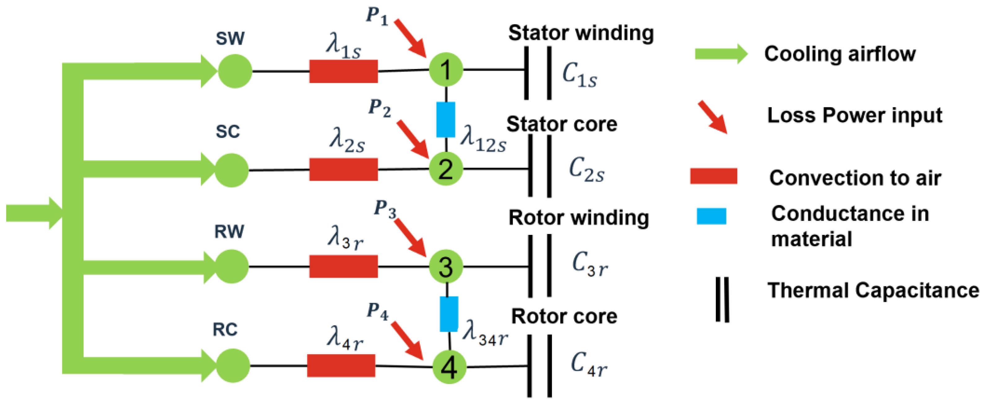
Appendix A. Parametrizing the Thermal Model

From a thermal point of view, the motor is modeled with four nodes: stator winding (node 1), stator core (node 2), rotor winding (node 3), and rotor core (node 4). The thermal equivalent network is illustrated in Figure A1 with thermal capacitances; it is connected to a power source and has thermal conductance among the nodes and to the cooling air.
Figure A1. Lumped-parameter thermal network model.
Values of the thermal capacitance C 1 s , C 2 s , C 3 r , and C 4 r are calculated analytically from the geometric and material information of the motor, where the indices 1s, 2s, 3r, and 4r refer to Node 1-Stator, Node 2-Stator, Node 3-Rotor, and Node 4-Rotor respectively. The capacitance for stator yoke C 1 s is the sum of the capacitance of stator housing, stator back iron, stator tooth, and flange mounting [36]. The stator winding capacitance C 2 s includes the capacitance for the stator winding and the end winding capacitances. The capacitance for stator yoke C 1 r is the sum of the capacitance of the rotor yoke and rotor bars. The rotor winding capacitance C 2 r includes the capacitance for the rotor winding and the end winding capacitances. The thermal conductance λ1s, λ2s, λ3r, and λ4r vary with the airflow due to the convection. The model shown in Figure A1 can be represented mathematically by the following first-order differential system:
P 1 = C 1 s d T 1 dt + λ 1 s T 1 T env + λ 12 s T 1 T 2 ,
P 2 = C 2 s d T 2 dt + λ 2 s T 2 T env + λ 12 s T 2 T 1 ,
P 3 = C 3 r d T 3 dt + λ 3 r ( T 3 T env ) + λ 34 r ( T 3 T 4 ) ,
P 4 = C 4 r d T 4 dt + λ 4 r ( T 4 T env ) + λ 34 r ( T 4 T 3 ) ,
where Ti is the temperature at the corresponding node i. The temperatures of the cooling air at the four nodes (marked as SW, SC, RW, and RC in Figure A1) are assigned to the environmental (or ambient) temperature T env .
The losses at the four nodes in Figure A1 are distributed as shown in Table A1 and they can be calculated as follows:
P 1 = K s t e m p P c u 1 + K s t r a y P s t r a y + K h a r m P h a r m ,
P 2 = K P f e P f e ,
P 3 = K r t e m p P c u 2 + ( 1 K s t r a y ) P s t r a y + ( 1 K h a r m ) P h a r m ,
P 4 = ( 1 K P f e ) P f e ,
where P c u 1 , P c u 2 , P s t r a y , P h a r m , and P f e are the stator copper loss, rotor copper loss, stray loss, harmonic loss, and iron loss, respectively. The coefficients K s t e m p , K r t e m p , K s t r a y , K h a r m and K P f e are the corresponding loss coefficients.
Table A1. Distribution of losses in the LPTN model (x denotes a connection between the corresponding row and column).
NodeWinding LossesStray LossesHarmonic LossesIron Losses
1xxx
2 x
3xxx
4 x
The losses in Equations (A5)–(A8) can be calculated as follows [8,37,38,39]:
P c u 1 = R 1 I 1 2 ,
P c u 2 = R 21 I 21 2 ,
P s t r a y = P S U P f f n o m 1.5 I 1 I 1 , n o m   2 ,
P f e = K f   f α B m a x β ,
where I 1 , and I 21 are the stator and rotor currents, respectively, and R1 and R2 are the stator and rotor winding resistances, respectively, which depend on the temperature according to following equations:
R 1 = R 1,20 ( 1 + α R 1 ( T 1 20 ) ) ,
R 21 = R 21,20 ( 1 + α R 2 ( T 3 20 ) ) ,
where R 1,20 and R 21,20 are the stator and rotor winding resistances at 20 °C, and α R 1 and α R 21 are the temperature coefficients of the stator and rotor, respectively. In Equation (A11), f is the stator frequency with a nominal value fnom, I1 is the stator current with a nominal value I1,nom, and PSUP is the equivalent-rated input power. In Equation (A12), Kf is a constant that depends on the material properties and the core geometry, f is the frequency of the magnetic field, Bmax is the peak magnetic flux density in the core, and α and β are empirically determined constants. The harmonic losses P h a r m o are measured at a few operation points and included as a look-up table in the loss model.

References

  1. Fathy Abouzeid, A.; Guerrero, J.M.; Endemaño, A.; Muniategui, I.; Ortega, D.; Larrazabal, I.; Briz, F. Control strategies for induction motors in railway traction applications. Energies 2020, 13, 700. [Google Scholar] [CrossRef]
  2. Hannan, M.A.; Ali, J.A.; Mohamed, A.; Hussain, A. Optimization techniques to enhance the performance of induction motor drives: A review. Renew. Sustain. Energy Rev. 2018, 81, 1611–1626. [Google Scholar] [CrossRef]
  3. Lemmens, J.; Vanassche, P.; Driesen, J. Optimal control of traction motor drives under electrothermal constraints. IEEE J. Emerg. Sel. Top. Power Electron. 2014, 2, 249–263. [Google Scholar] [CrossRef]
  4. Dorrell, D.G. Combined thermal and electromagnetic analysis of permanent-magnet and induction machines to aid calculation. IEEE Trans. Ind. Electron. 2008, 55, 3566–3574. [Google Scholar] [CrossRef]
  5. Ramakrishnan, R.; Islam, R.; Islam, M.; Sebastian, T. Real time estimation of parameters for controlling and monitoring permanent magnet synchronous motors. In Proceedings of the 2009 IEEE International Electric Machines and Drives Conference, Miami, FL, USA, 3–6 May 2009; pp. 1194–1199. [Google Scholar]
  6. Wilson, S.D.; Stewart, P.; Taylor, B.P. Methods of resistance estimation in permanent magnet synchronous motors for real-time thermal management. IEEE Trans. Energy Convers. 2010, 25, 698–707. [Google Scholar] [CrossRef]
  7. Wallscheid, O. Thermal monitoring of electric motors: State-of-the-art review and future challenges. IEEE Open J. Ind. Appl. 2021, 2, 204–223. [Google Scholar] [CrossRef]
  8. Kral, C.; Haumer, A.; Lee, S.B. A practical thermal model for the estimation of permanent magnet and stator winding temperatures. IEEE Trans. Power Electron. 2013, 29, 455–464. [Google Scholar] [CrossRef]
  9. Sciascera, C.; Giangrande, P.; Papini, L.; Gerada, C.; Galea, M. Analytical thermal model for fast stator winding temperature prediction. IEEE Trans. Ind. Electron. 2017, 64, 6116–6126. [Google Scholar] [CrossRef]
  10. Zhu, Y.; Xiao, M.; Lu, K.; Wu, Z.; Tao, B. A simplified thermal model and online temperature estimation method of permanent magnet synchronous motors. Appl. Sci. 2019, 9, 3158. [Google Scholar] [CrossRef]
  11. Guemo, G.G.; Chantrenne, P.; Jac, J. Parameter identification of a lumped parameter thermal model for a permanent magnet synchronous machine. In Proceedings of the 2013 International Electric Machines & Drives Conference, Chicago, IL, USA, 12–15 May 2013; pp. 1316–1320. [Google Scholar]
  12. Huber, T.; Peters, W.; Böcker, J. Monitoring critical temperatures in permanent magnet synchronous motors using low-order thermal models. In Proceedings of the 2014 International Power Electronics Conference (IPEC-Hiroshima 2014-ECCE ASIA), Hiroshima, Japan, 18–21 May 2014; IEEE: Piscataway, NJ, USA, 2014. [Google Scholar]
  13. Gedlu, E.G.; Wallscheid, O.; Böcker, J. Permanent magnet synchronous machine temperature estimation using low-order lumped-parameter thermal network with extended iron loss model. In Proceedings of the 10th International Conference on Power Electronics, Machines and Drives (PEMD 2020), Online Conference, 15–17 December 2020; IET: London, UK, 2020. [Google Scholar]
  14. Wallscheid, O.; Böcker, J. Global identification of a low-order lumped-parameter thermal network for permanent magnet synchronous motors. IEEE Trans. Energy Convers. 2015, 31, 354–365. [Google Scholar] [CrossRef]
  15. Xiao, S.; Griffo, A. Online thermal parameter identification for permanent magnet synchronous machines. IET Electr. Power Appl. 2020, 14, 2340–2347. [Google Scholar] [CrossRef]
  16. Kirchgässner, W.; Wallscheid, O.; Böcker, J. Data-driven permanent magnet temperature estimation in synchronous motors with supervised machine learning: A benchmark. IEEE Trans. Energy Convers. 2021, 36, 2059–2067. [Google Scholar] [CrossRef]
  17. Zhang, S.; Wallscheid, O.; Porrmann, M. Machine learning for the control and monitoring of electric machine drives: Advances and trends. IEEE Open J. Ind. Appl. 2023, 4, 188–214. [Google Scholar] [CrossRef]
  18. Kirchgässner, W.; Wallscheid, O.; Böcker, J. Empirical evaluation of exponentially weighted moving averages for simple linear thermal modeling of permanent magnet synchronous machines. In Proceedings of the 2019 IEEE 28th International Symposium on Industrial Electronics (ISIE), Vancouver, BC, Canada, 12–14 June 2019; IEEE: Piscataway, NJ, USA, 2019; pp. 318–323. [Google Scholar]
  19. Nogay, H.S. Prediction of internal temperature in stator winding of three-phase induction motors with ann. Eur. Trans. Electr. Power 2011, 21, 120–128. [Google Scholar] [CrossRef]
  20. Wallscheid, O.; Kirchgässner, W.; Böcker, J. Investigation of long short-term memory networks to temperature prediction for permanent magnet synchronous motors. In Proceedings of the 2017 International Joint Conference on Neural Networks (IJCNN), Anchorage, AK, USA, 14–19 May 2017; IEEE: Piscataway, NJ, USA, 2017; pp. 1940–1947. [Google Scholar]
  21. Kirchgässner, W.; Wallscheid, O.; Böcker, J. Deep residual convolutional and recurrent neural networks for temperature estimation in permanent magnet synchronous motors. In Proceedings of the 2019 IEEE International Electric Machines & Drives Conference (IEMDC), San Diego, CA, USA, 12–15 May 2019; IEEE: Piscataway, NJ, USA, 2019. [Google Scholar]
  22. Kirchgässner, W.; Wallscheid, O.; Böcker, J. Thermal neural networks: Lumped-parameter thermal modeling with state-space machine learning. Eng. Appl. Artif. Intell. 2023, 117, 105537. [Google Scholar] [CrossRef]
  23. Wlas, M.; Krzeminski, Z.; Toliyat, H.A. Neural-network-based parameter estimations of induction motors. IEEE Trans. Ind. Electron. 2008, 55, 1783–1794. [Google Scholar] [CrossRef]
  24. Rafaq, M.S.; Jung, J.W. A comprehensive review of state-of-the-art parameter estimation techniques for permanent magnet synchronous motors in wide speed range. IEEE Trans. Ind. Inform. 2019, 16, 4747–4758. [Google Scholar] [CrossRef]
  25. Harashima, F.; Demizu, Y.; Kondo, S.; Hashimoto, H. Application of neutral networks to power converter control. In Proceedings of the Conference Record of the IEEE Industry Applications Society Annual Meeting, San Diego, CA, USA, 1–5 October 1989; IEEE: Piscataway, NJ, USA, 1989; pp. 1086–1091. [Google Scholar]
  26. Wishart, M.T.; Harley, R.G. Identification and control of induction machines using artificial neural networks. IEEE Trans. Ind. Appl. 1995, 31, 612–619. [Google Scholar] [CrossRef]
  27. Rahman, M.A.; Hoque, M.A. On-line adaptive artificial neural network based vector control of permanent magnet synchronous motors. IEEE Trans. Energy Convers. 1998, 13, 311–318. [Google Scholar]
  28. Yi, Y.; Vilathgamuwa, D.M.; Rahman, M.A. Implementation of an artificial-neural-network-based real-time adaptive controller for an interior permanent-magnet motor drive. IEEE Trans. Ind. Appl. 2003, 39, 96–104. [Google Scholar]
  29. Zhang, Q.; Zeng, W.; Lin, Q.; Chng, C.B.; Chui, C.K.; Lee, P.S. Deep reinforcement learning towards real-world dynamic thermal management of data centers. Appl. Energy 2023, 333, 120561. [Google Scholar] [CrossRef]
  30. Egan, D.; Zhu, Q.; Prucka, R. A Review of Reinforcement Learning-Based Powertrain Controllers: Effects of Agent Selection for Mixed-Continuity Control and Reward Formulation. Energies 2023, 16, 3450. [Google Scholar] [CrossRef]
  31. Zhang, Y.; Huang, J.; He, L.; Zhao, D.; Zhao, Y. Reinforcement learning-based control for the thermal management of the battery and occupant compartments of electric vehicles. Sustain. Energy Fuels 2024, 8, 588–603. [Google Scholar] [CrossRef]
  32. Book, G.; Traue, A.; Balakrishna, P.; Brosch, A.; Schenke, M.; Hanke, S.; Kirchgässner, W.; Wallscheid, O. Transferring online reinforcement learning for electric motor control from simulation to real-world experiments. IEEE Open J. Power Electron. 2021, 2, 187–201. [Google Scholar] [CrossRef]
  33. Traue, A.; Book, G.; Kirchgässner, W.; Wallscheid, O. Toward a reinforcement learning environment toolbox for intelligent electric motor control. IEEE Trans. Neural Netw. Learn. Syst. 2020, 33, 919–928. [Google Scholar] [CrossRef]
  34. Bhattacharjee, S.; Halder, S.; Balamurali, A.; Towhidi, M.; Iyer, L.V.; Kar, N.C. An advanced policy gradient based vector control of PMSM for EV application. In Proceedings of the 2020 10th International Electric Drives Production Conference (EDPC), Ludwigsburg, Germany, 8–9 December 2020; IEEE: Piscataway, NJ, USA, 2020; pp. 1–5. [Google Scholar]
  35. Fattouh, A.; Sahoo, S. Data-driven reinforcement learning-based parametrization of a thermal model in induction traction motors. In Proceedings of the 64th International Conference of Scandinavian Simulation Society, SIMS 2023, Västerås, Sweden, 25–28 September 2023; pp. 310–317. [Google Scholar]
  36. Wöckinger, D.; Bramerdorfer, G.; Drexler, S.; Vaschetto, S.; Cavagnino, A.; Tenconi, A.; Amrhein, W.; Jeske, F. Measurement-based optimization of thermal networks for temperature monitoring of outer rotor PM machines. In Proceedings of the 2020 IEEE Energy Conversion Congress and Exposition (ECCE), Detroit, MI, USA, 11–15 October 2020; pp. 4261–4268. [Google Scholar]
  37. Filizadeh, S. Electric Machines and Drives: Principles, Control, Modeling, and Simulation; CRC Press: Boca Raton, FL, USA, 2013. [Google Scholar]
  38. Maroteaux, A. Study of Analytical Models for Harmonic Losses Calculations in Traction Induction Motors; KTH, School of Electrical Engineering (EES): Stockholm, Sweden, 2016. [Google Scholar]
  39. Roshandel, E.; Mahmoudi, A.; Kahourzade, S.; Yazdani, A.; Shafiullah, G. Losses in efficiency maps of electric vehicles: An overview. Energies 2021, 14, 7805. [Google Scholar] [CrossRef]
Disclaimer/Publisher’s Note: The statements, opinions and data contained in all publications are solely those of the individual author(s) and contributor(s) and not of MDPI and/or the editor(s). MDPI and/or the editor(s) disclaim responsibility for any injury to people or property resulting from any ideas, methods, instructions or products referred to in the content.

Article Metrics

Citations

Article Access Statistics

Multiple requests from the same IP address are counted as one view.