

A Learnable Viewpoint Evolution Method for Accurate Pose Estimation of Complex Assembled Product

Abstract
Featured Application
Abstract
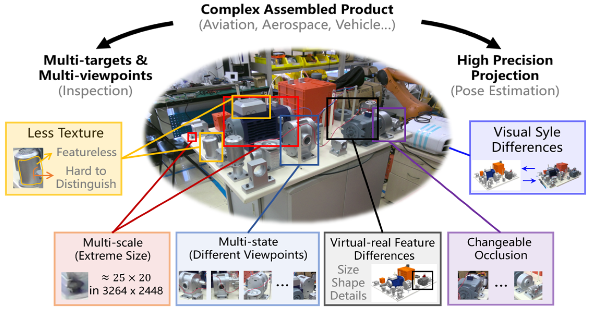
1. Introduction
- (1)
- Reconstruct the camera pose estimation into the evolution of parameter population to generate an interpretable fine-grained iterative framework;
- (2)
- To balance exploration and optimization, feasible region constraint, parent migration, and reproduction strategies are designed for local–global collaborative control;
- (3)
- Propose a guided-model-based hierarchical cyclic effective trajectory learning mechanism to reduce the empirical dependence of control and enhance adaptability.
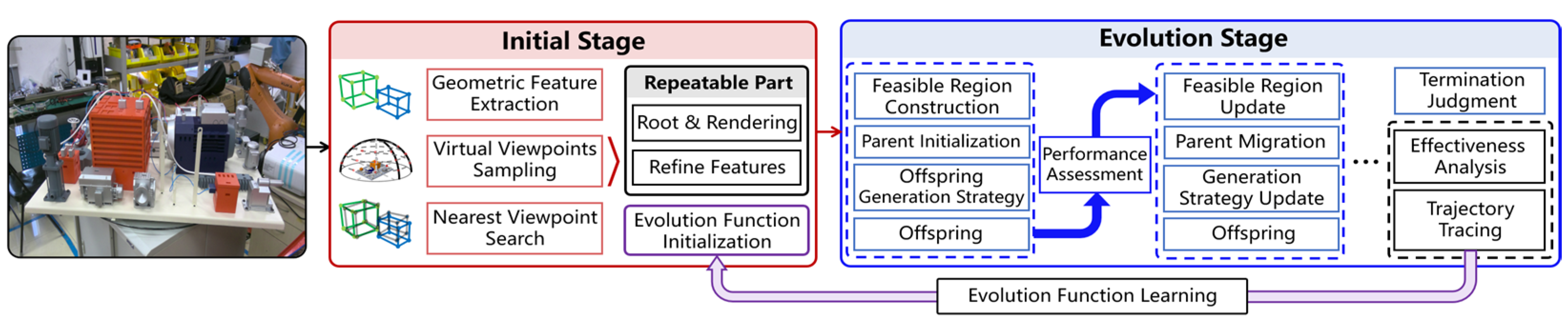
2. Proposed Method
2.1. Viewpoint Performance Assessment
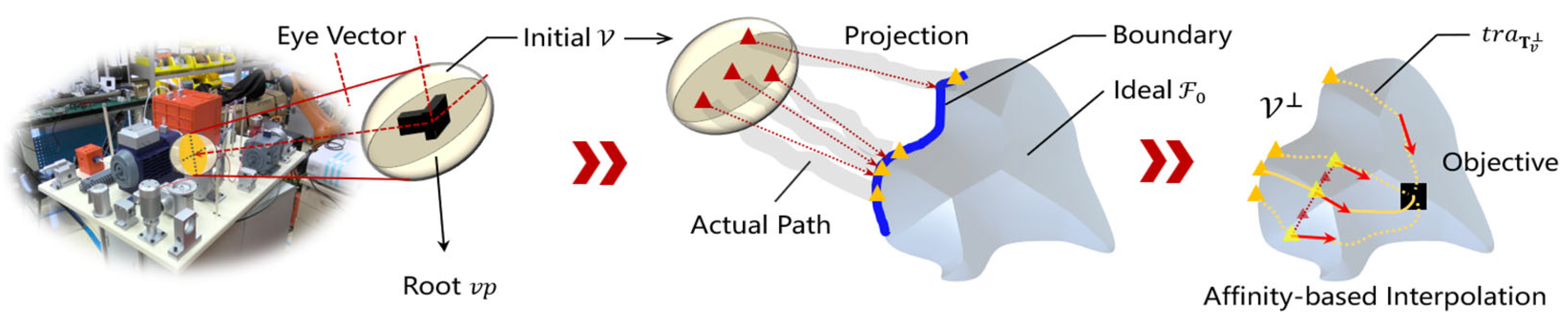
2.2. Feasible Region Construction and Update
2.2.1. Problem Planning
2.2.2. Initialization
2.2.3. Boundary Projection
2.2.4. Sparse Trajectory Approximation
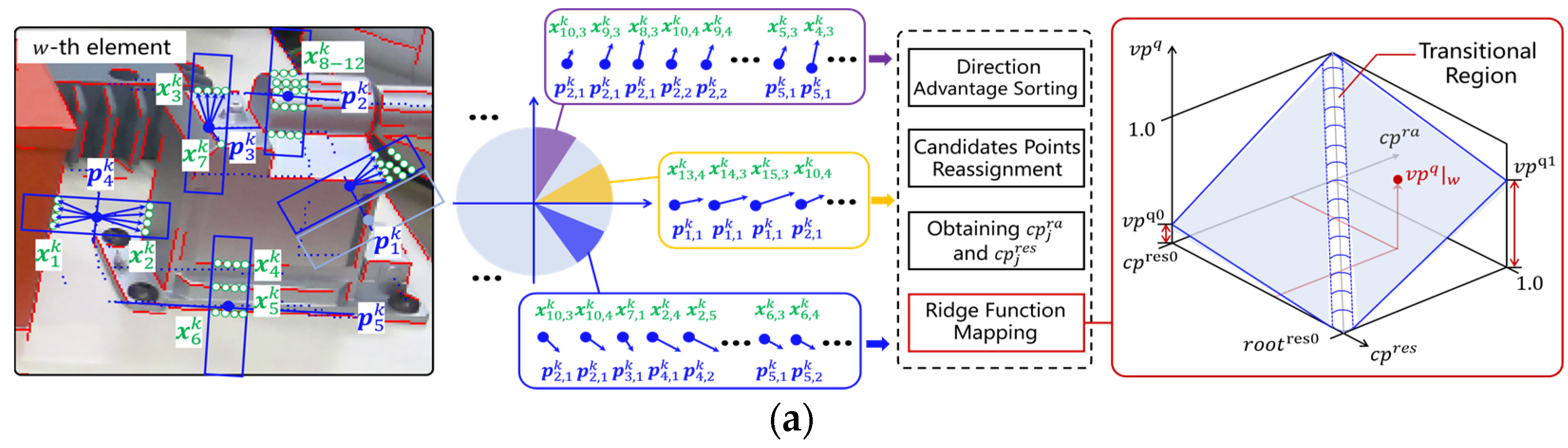
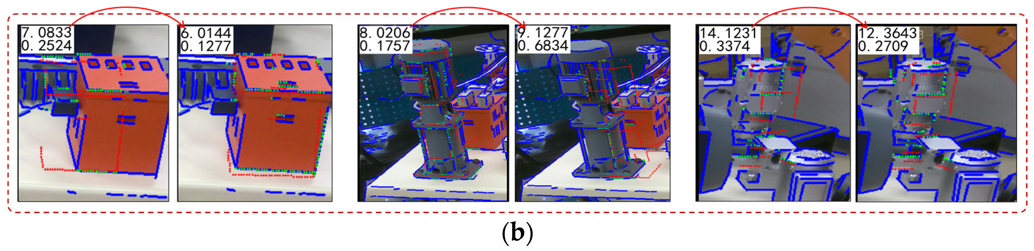
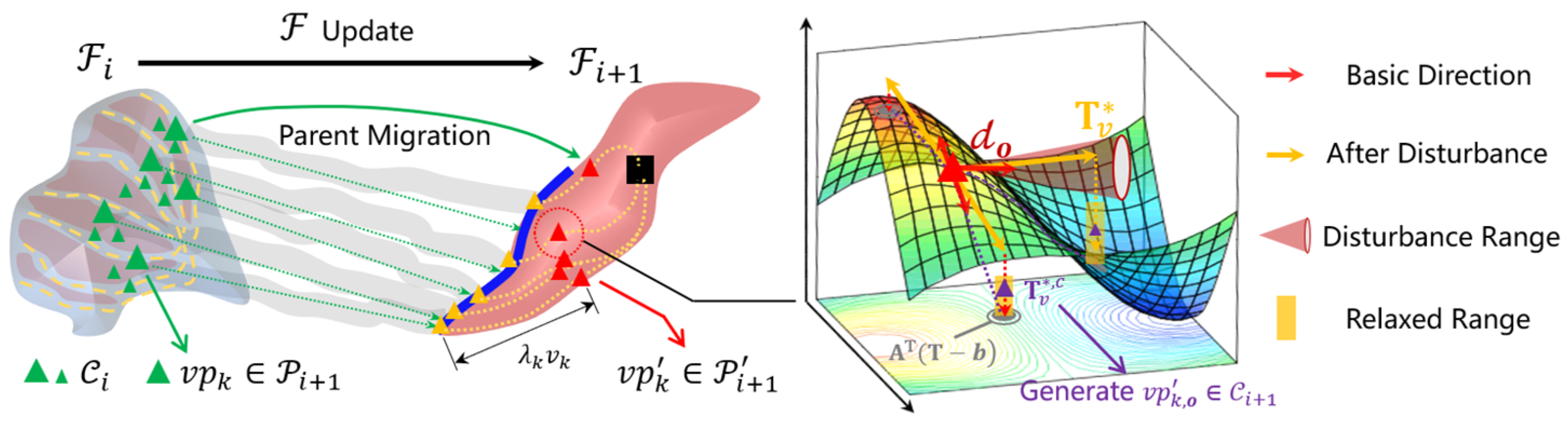
2.3. Parent Migration and Offspring Generation
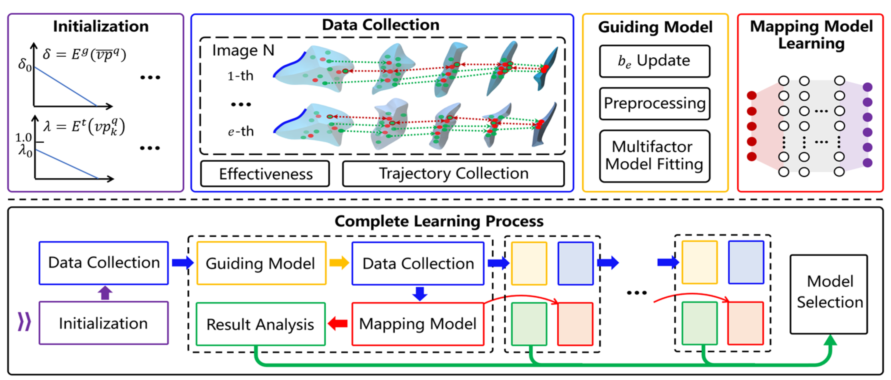
2.4. A Learnable Evolutionary Function Optimization
3. Experiment and Results
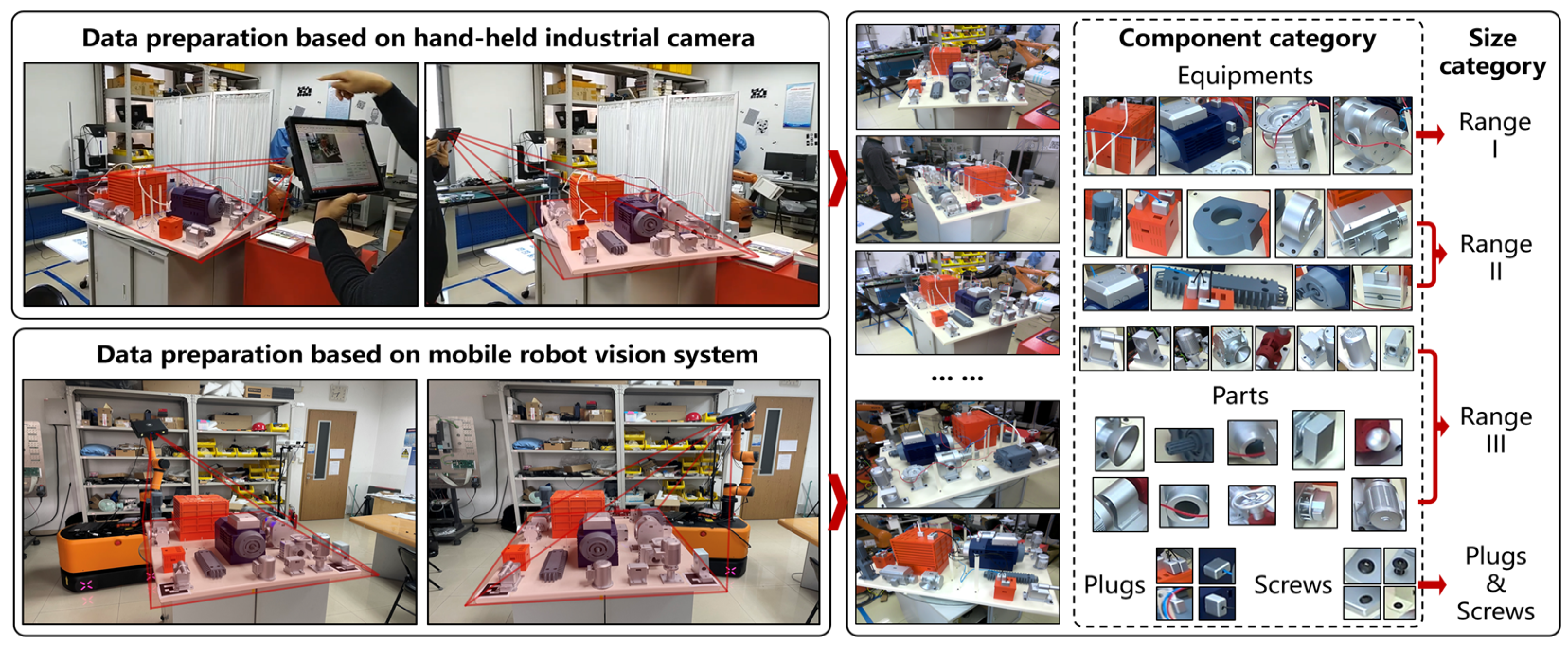
3.1. Preliminary Works
3.2. Performance of Pose Estimation
3.3. In-Depth Analysis of the Proposed Method
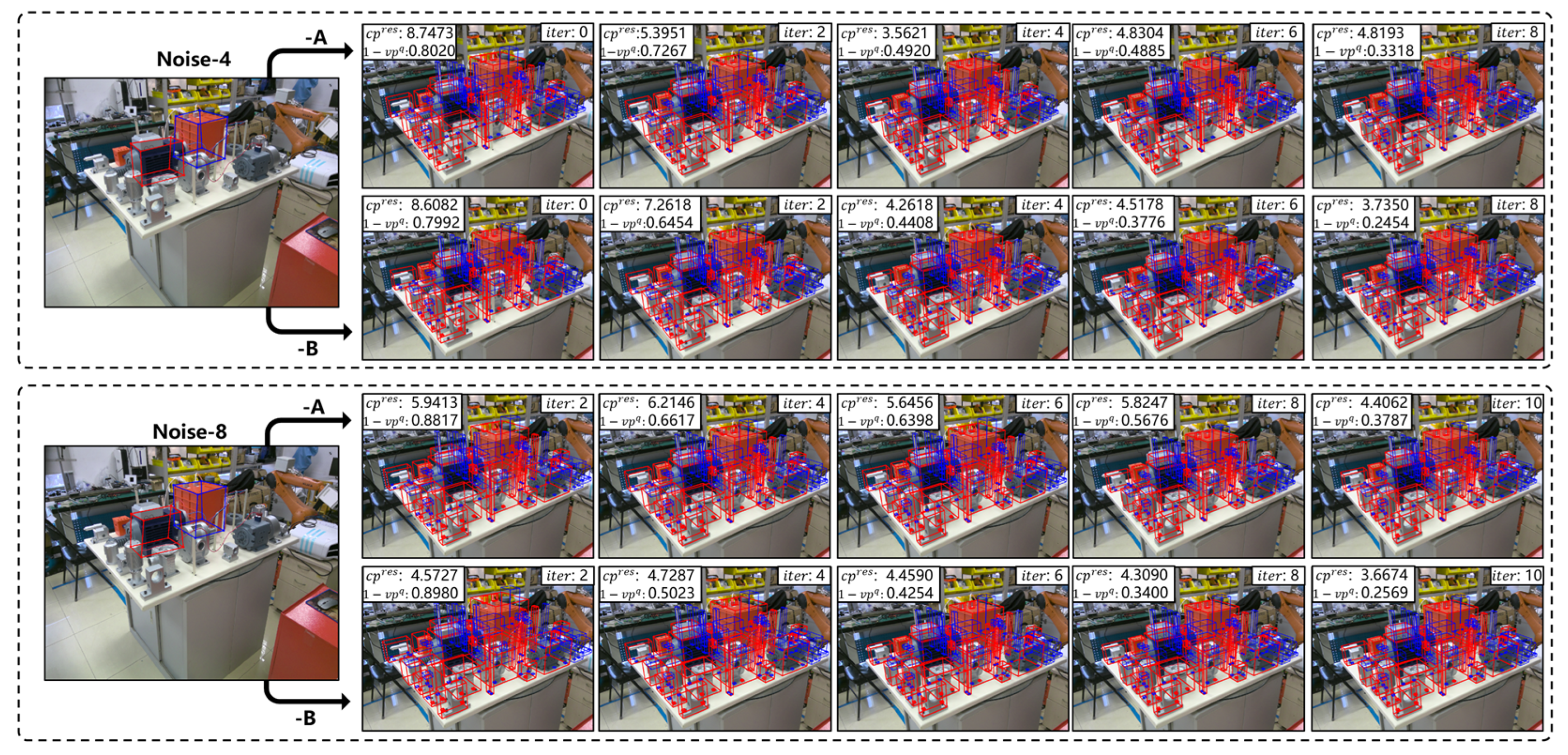
3.3.1. Verifying Robustness to Initial Pose Deviation
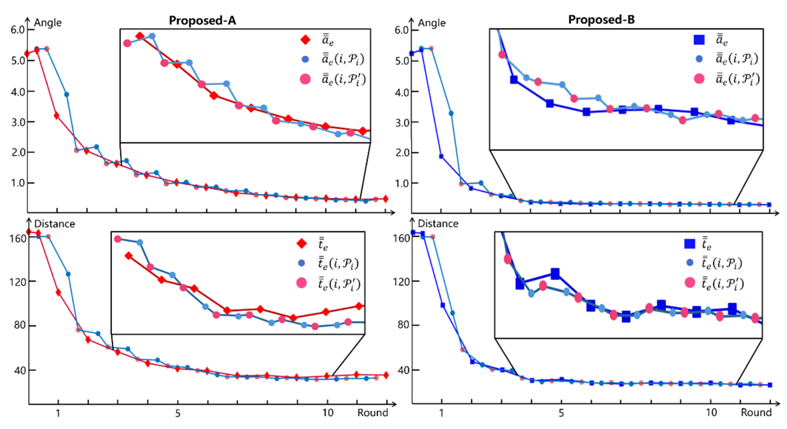
3.3.2. The Advantage of Learning Mechanism
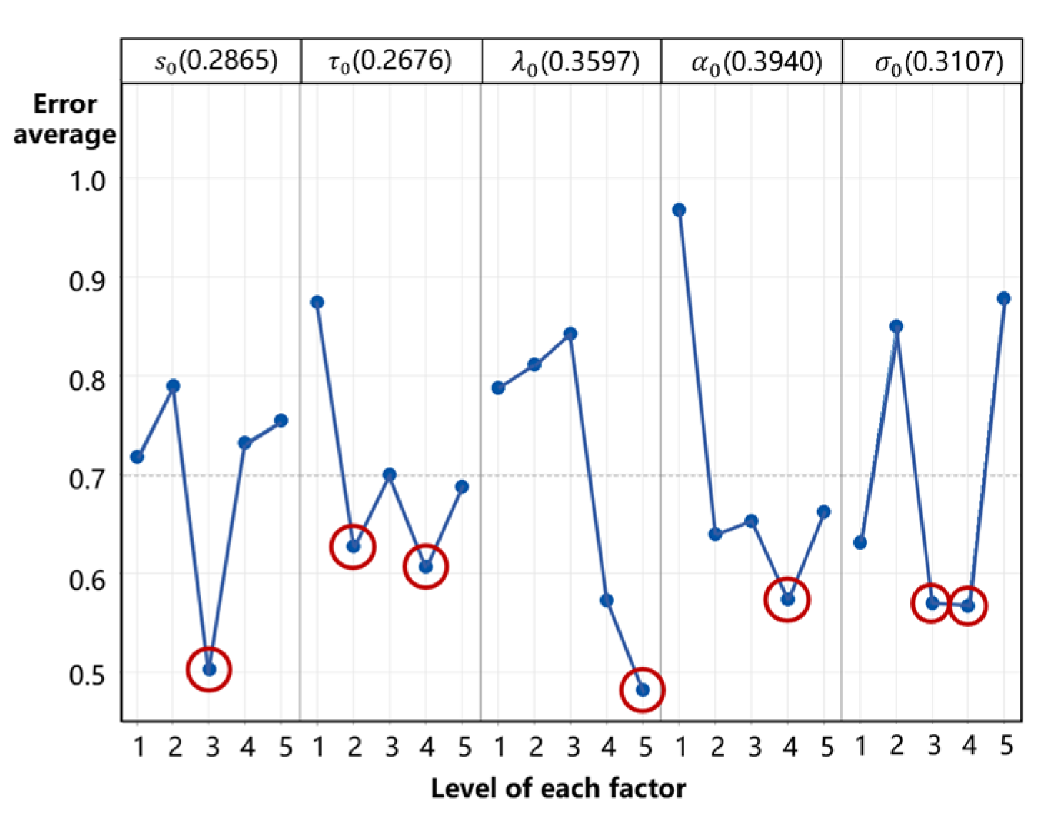
3.4. Parameter Sensitivity Analysis
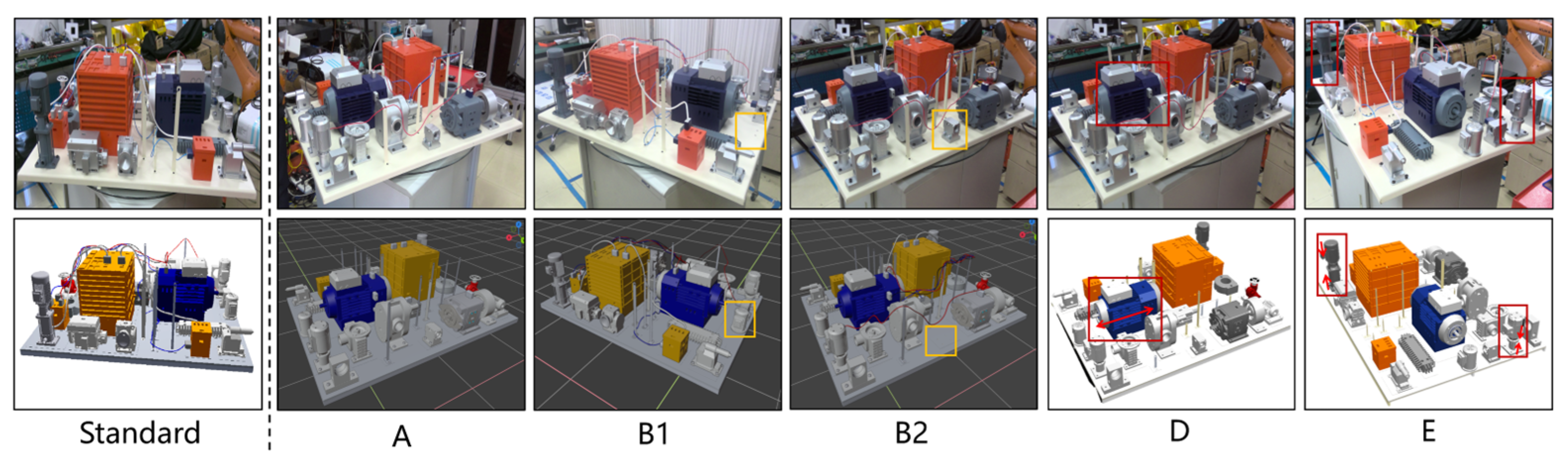
3.5. Appearance Difference Adaptability
3.6. Practical Application Cases
4. Discussion and Conclusions
- (1)
- A hierarchical architecture from coarse to fine is a practical approach to image-based pose estimation while maintaining high accuracy and reliability;
- (2)
- (3)
- Some practical problems, such as limited samples, complex structure, and multiple elements, make it difficult to directly perform complex advanced DL-based networks. On the contrary, indirect models that only require weak annotation are easier to deploy in practical applications;
- (4)
- For global or divide-and-conquer architectures based on matching, metric, and optimization, the coordination of exploration and optimization requires more detailed regulation in the pose estimation of complex assembled products.
Author Contributions
Funding
Institutional Review Board Statement
Informed Consent Statement
Data Availability Statement
Conflicts of Interest
References
- Marchand, E.; Uchiyama, H.; Spindler, F. Pose Estimation for Augmented Reality: A Hands-On Survey. IEEE Trans. Visual Comput. 2016, 22, 2633–2651. [Google Scholar] [CrossRef] [PubMed]
- Wang, Z.; Shang, Y.; Zhang, H. A Survey on Approaches of Monocular CAD Model-Based 3D Objects Pose Estimation and Tracking. In Proceedings of the 2018 IEEE CSAA Guidance, Navigation and Control Conference (CGNCC), Xiamen, China, 10–12 August 2018. [Google Scholar] [CrossRef]
- Jia, Z.; Wang, M.; Zhao, S. A review of deep learning-based approaches for defect detection in smart manufacturing. J. Opt. 2024, 53, 1345–1351. [Google Scholar] [CrossRef]
- Eswaran, M.; Gulivindala, A.K.; Inkulu, A.K.; Bahubalendruni, M.R. Augmented reality-based guidance in product assembly and maintenance/repair perspective: A state of the art review on challenges and opportunities. Expert Syst. Appl. 2023, 213, 118983. [Google Scholar] [CrossRef]
- Hao, J.C.; He, D.; Li, Z.Y.; Hu, P.; Chen, Y.; Tang, K. Efficient cutting path planning for a non-spherical tool based on an iso-scallop height distance field. Chin. J. Aeronaut. 2023, in press. [Google Scholar] [CrossRef]
- Glorieux, E.; Franciosa, P.; Ceglarek, D. Coverage path planning with targeted viewpoint sampling for robotic free-form surface inspection. Robot. Comput. Integr. Manuf. 2020, 61, 101843. [Google Scholar] [CrossRef]
- Du, G.; Wang, K.; Lian, S.; Zhao, K. Vision-based robotic grasping from object localization, object pose estimation to grasp estimation for parallel grippers: A review. Artif. Intell. Rev. 2021, 54, 1677–1734. [Google Scholar] [CrossRef]
- Wang, H.Y.; Shen, Q.; Deng, Z.L.; Cao, X.; Wang, X. Absolute pose estimation of UAV based on large-scale satellite image. Chin. J. Aeronaut. 2023, in press. [CrossRef]
- Zhang, M.; Zhang, C.C.; Wang, W.; Du, R.; Meng, S. Research on Automatic Assembling Method of Large Parts of Spacecraft Based on Vision Guidance. In Proceedings of the 2021 2nd International Conference on Artificial Intelligence and Information Systems, ACM, Chongqing, China, 28–30 May 2021. [Google Scholar] [CrossRef]
- Qin, L.; Wang, T. Design and research of automobile anti-collision warning system based on monocular vision sensor with license plate cooperative target. Multimed. Tools Appl. 2017, 76, 14815–14828. [Google Scholar] [CrossRef]
- Jiang, C.; Li, W.; Li, W.; Wang, D.F.; Zhu, L.J.; Xu, W.; Zhao, H.; Ding, H. A Novel Dual-Robot Accurate Calibration Method Using Convex Optimization and Lie Derivative. IEEE Trans. Robot. 2024, 40, 960–977. [Google Scholar] [CrossRef]
- Huang, B.; Tang, Y.; Ozdemir, S.; Ling, H. A Fast and Flexible Projector-Camera Calibration System. IEEE Trans. Autom. Sci. Eng. 2021, 18, 1049–1063. [Google Scholar] [CrossRef]
- Nubiola, A.; Bonev, I.A. Absolute calibration of an ABB IRB 1600 robot using a laser tracker. Robot. Comput. Integr. Manuf. 2012, 29, 236–245. [Google Scholar] [CrossRef]
- Yu, H.; Huang, Y.; Zheng, D.; Bai, L.; Han, J. Three-dimensional shape measurement technique for large-scale objects based on line structured light combined with industrial robot. Optik 2020, 202, 163656. [Google Scholar] [CrossRef]
- Li, D.; Wang, H.; Liu, N.; Wang, X.; Xu, J. 3D Object Recognition and Pose Estimation from Point Cloud Using Stably Observed Point Pair Feature. IEEE Access 2020, 8, 44335–44345. [Google Scholar] [CrossRef]
- Wuest, H.; Vial, F.; Stricker, D. Adaptive line tracking with multiple hypotheses for augmented reality. In Proceedings of the Fourth IEEE and ACM International Symposium on Mixed and Augmented Reality (ISMAR’05), Vienna, Austria, 5–8 October 2005; pp. 62–69. [Google Scholar] [CrossRef]
- Han, P.; Zhao, G. A review of edge-based 3D tracking of rigid objects. Virtual Real. Intell. Hardw. 2019, 1, 580–596. [Google Scholar] [CrossRef]
- Huang, H.; Zhong, F.; Sun, Y.; Qin, X. An Occlusion-aware Edge-Based Method for Monocular 3D Object Tracking using Edge Confidence. Comput. Graph. Forum 2020, 39, 399–409. [Google Scholar] [CrossRef]
- Jau, Y.-Y.; Zhu, R.; Su, H.; Chandraker, M. Deep keypoint-based camera pose estimation with geometric constraints. In Proceedings of the 2020 IEEE/RSJ International Conference on Intelligent Robots and Systems (IROS), Las Vegas, NV, USA, 24 October 2020–24 January 2021; pp. 4950–4957. [Google Scholar] [CrossRef]
- Lepetit, V.; Moreno-Noguer, F.; Fua, P. EPnP: An accurate O(n) solution to the PnP problem. Int. J. Comput. Vis. 2009, 81, 155–166. [Google Scholar] [CrossRef]
- Ferraz, L.; Binefa, X.; Moreno-Noguer, F. Leveraging Feature Uncertainty in the PnP Problem. In Proceedings of the British Machine Vision Conference 2014, British Machine Vision Association, Nottingham, UK, 1 September 2014. [Google Scholar] [CrossRef]
- Zheng, Y.; Sugimoto, S.; Okutomi, M. ASPnP: An Accurate and Scalable Solution to the Perspective-n-Point Problem. Trans. Inf. Syst. 2013, 96, 1525–1535. [Google Scholar] [CrossRef]
- Garro, V.; Crosilla, F.; Fusiello, A. Solving the PnP Problem with Anisotropic Orthogonal Procrustes Analysis. In Proceedings of the 2012 Second International Conference on 3D Imaging, Modeling, Processing, Visualization & Transmission, Zurich, Switzerland, 13–15 October 2012. [Google Scholar] [CrossRef]
- Urban, S.; Leitloff, J.; Hinz, S. MLPnP-A Real-Time Maximum Likelihood Solution to the Perspective-n-Point Problem. ISPRS Ann. Photogramm. Remote Sens. Spat. Inf. Sci. 2016, III-3, 131–138. [Google Scholar] [CrossRef]
- Arandjelovic, R.; Gronat, P.; Torii, A.; Pajdla, T.; Sivic, J. NetVLAD: CNN Architecture for Weakly Supervised Place Recognition. IEEE Trans. Pattern Anal. Mach. Intell. 2018, 40, 1437–1451. [Google Scholar] [CrossRef]
- Gordo, A.; Almazán, J.; Revaud, J.; Larlus, D. Deep Image Retrieval: Learning Global Representations for Image Search. In Computer Vision—ECCV 2016; Leibe, B., Matas, J., Sebe, N., Welling, M., Eds.; Springer International Publishing: Cham, Switzerland, 2016. [Google Scholar] [CrossRef]
- Humenberger, M.; Cabon, Y.; Guerin, N.; Morat, J.; Leroy, V.; Revaud, J.; Rerole, P.; Pion, N.; de Souza, C.; Csurka, G. Robust Image Retrieval-based Visual Localization using Kapture. arXiv 2022, arXiv:2007.13867. [Google Scholar]
- Kendall, A.; Grimes, M.; Cipolla, R. PoseNet: A Convolutional Network for Real-Time 6-DOF Camera Relocalization. In Proceedings of the 2015 IEEE International Conference on Computer Vision (ICCV), Santiago, Chile, 7–13 December 2015. [Google Scholar] [CrossRef]
- Kendall, A.; Cipolla, R. Geometric Loss Functions for Camera Pose Regression with Deep Learning. In Proceedings of the 2017 IEEE Conference on Computer Vision and Pattern Recognition (CVPR), Honolulu, HI, USA, 21–26 July 2017. [Google Scholar] [CrossRef]
- Peng, S.; Liu, Y.; Huang, Q.; Zhou, X.; Bao, H. PVNet: Pixel-wise voting network for 6dof pose estimation. IEEE Trans. Pattern Anal. Mach. Intell. 2022, 44, 3212–3223. [Google Scholar] [CrossRef] [PubMed]
- Balntas, V.; Li, S.; Prisacariu, V. RelocNet: Continuous Metric Learning Relocalisation Using Neural Nets. In Computer Vision-ECCV 2018; Ferrari, V., Hebert, M., Sminchisescu, C., Weiss, Y., Eds.; Springer International Publishing: Cham, Switzerland, 2018. [Google Scholar] [CrossRef]
- Xu, Y.; Lin, K.-Y.; Zhang, G.; Wang, X.; Li, H. RNNPose: Recurrent 6-DoF Object Pose Refinement with Robust Correspondence Field Estimation and Pose Optimization. In Proceedings of the 2022 IEEE/CVF Conference on Computer Vision and Pattern Recognition (CVPR), New Orleans, LA, USA, 18–24 June 2022. [Google Scholar]
- Bukschat, Y.; Vetter, M. EfficientPose-An efficient, accurate and scalable end-to-end 6D multi object pose estimation approach. arXiv 2020, arXiv:2011.04307. [Google Scholar]
- Labbe, Y.; Manuelli, L.; Mousavian, A.; Tyree, S.; Birchfield, S.; Tremblay, J.; Carpentier, J.; Aubry, M.; Fox, D.; Sivic, J. Megapose: 6d pose estimation of novel objects via render & compare. arXiv 2022, arXiv:2212.06870. [Google Scholar]
- Brachmann, E.; Krull, A.; Michel, F.; Gumhold, S.; Shotton, J.; Rother, C. Learning 6D Object Pose Estimation Using 3D Object Coordinates. In Computer Vision—ECCV 2014; Lecture Notes in Computer Science; Springer: Cham, Switzerland, 2014; Volume 8690. [Google Scholar] [CrossRef]
- Brachmann, E.; Krull, A.; Nowozin, S.; Shotton, J.; Michel, F.; Gumhold, S.; Rother, C. DSAC-Differentiable RANSAC for Camera Localization. In Proceedings of the 2017 IEEE Conference on Computer Vision and Pattern Recognition (CVPR), Honolulu, HI, USA, 21–26 July 2017. [Google Scholar] [CrossRef]
- Sarlin, P.-E.; Cadena, C.; Siegwart, R.; Dymczyk, M. From Coarse to Fine: Robust Hierarchical Localization at Large Scale. In Proceedings of the 2019 IEEE/CVF Conference on Computer Vision and Pattern Recognition (CVPR), Long Beach, CA, USA, 15–20 June 2019. [Google Scholar] [CrossRef]
- Ben Abdallah, H.; Jovančević, I.; Orteu, J.-J.; Brèthes, L. Automatic Inspection of Aeronautical Mechanical Assemblies by Matching the 3D CAD Model and Real 2D Images. J. Imaging 2019, 5, 81. [Google Scholar] [CrossRef] [PubMed]
- Liu, Y.; De, D.L.; Wei, B.; Chen, L.; Martin, R.R. Regularization Based Iterative Point Match Weighting for Accurate Rigid Transformation Estimation. IEEE Trans. Vis. Comput. Graph. 2015, 21, 1058–1071. [Google Scholar] [CrossRef] [PubMed]
- Hanna, J.P.; Niekum, S.; Stone, P. Importance sampling in reinforcement learning with an estimated behavior policy. Mach. Learn. 2021, 110, 1267–1317. [Google Scholar] [CrossRef]
- Tjaden, H.; Schwanecke, U.; Schömer, E. Real-time monocular pose estimation of 3d objects using temporally consistent local color histograms. In Proceedings of the IEEE International Conference on Computer Vision, Institute of Electrical and Electronics Engineers Inc., Venice, Italy, 22–29 October 2017. [Google Scholar] [CrossRef]
- Carlile, B.; Delamarter, G.; Kinney, P.; Marti, A.; Whitney, B. Improving Deep Learning by Inverse Square Root Linear Units (ISRLUs). arXiv 2017, arXiv:1710.09967. [Google Scholar]
- Gill, P.E.; Wong, E. Sequential Quadratic Programming Methods. In Mixed Integer Nonlinear Programming; Lee, J., Leyffer, S., Eds.; Springer: New York, NY, USA, 2012; pp. 147–224. [Google Scholar] [CrossRef]
- Schmid, A.; Biegler, L.T. Reduced Hessian Successive Quadratic Programming for Realtime Optimization. IFAC Proc. Vol. 1994, 27, 173–178. [Google Scholar] [CrossRef]
- Huang, H.; Zhong, F.; Qin, X. Pixel-Wise Weighted Region-Based 3D Object Tracking Using Contour Constraints. IEEE Trans. Visual Comput. Graph. 2022, 28, 4319–4331. [Google Scholar] [CrossRef]
- Zhang, J.; Yao, Y.; Deng, B. Fast and Robust Iterative Closest Point. IEEE Trans. Pattern Anal. Mach. Intell. 2022, 44, 3450–3466. [Google Scholar] [CrossRef]
- Tekin, B.; Sinha, S.N.; Fua, P. Real-Time Seamless Single Shot 6D Object Pose Prediction. In Proceedings of the 2018 IEEE/CVF Conference on Computer Vision and Pattern Recognition (CVPR), Salt Lake City, UT, USA, 18–23 June 2018. [Google Scholar] [CrossRef]
- Wang, Q.; Zhou, J.; Li, Z.; Sun, X.; Yu, Q. Robust and Accurate Monocular Pose Tracking for Large Pose Shift. IEEE Trans. Ind. Electron. 2023, 70, 8163–8173. [Google Scholar] [CrossRef]
- Tian, X.; Lin, X.; Zhong, F.; Qin, X. Large-Displacement 3D Object Tracking with Hybrid Non-local Optimization. In Proceedings of the Computer Vision-ECCV 2022: 17th European Conference, Tel Aviv, Israel, 23–27 October 2022. [Google Scholar] [CrossRef]
- Stoiber, M.; Pfanne, M.; Strobl, K.H.; Triebel, R.; Albu-Schäffer, A. A sparse gaussian approach to region-based 6DoF object tracking. In Proceedings of the Computer Vision-ACCV 2020: 15th Asian Conference on Computer Vision, Kyoto, Japan, 30 November 2020. [Google Scholar] [CrossRef]


| Range I () | Range II () | Range III () | Plugs () | Screws () | Average Error | ||||
|---|---|---|---|---|---|---|---|---|---|
| (°) | (mm) | ||||||||
| Rough pose | 0.64 | 0.57 | 0.34 | 0.11 | 0.02 | 6.03 | 185.71 | ||
| Group I | S4 + ASPnP | 0.74 | 0.60 | 0.43 | 0.13 | 0.03 | 3.61 | 134.74 | |
| Group II | FRICP + EPnP | 0.77 | 0.63 | 0.48 | 0.15 | 0.04 | 1.89 | 110.77 | |
| EPnP | S3 | 0.81 | 0.69 | 0.53 | 0.22 | 0.08 | 1.83 | 96.92 | |
| VPS | 0.86 | 0.75 | 0.62 | 0.32 | 0.18 | 1.44 | 85.23 | ||
| CEPnP | S3 | 0.79 | 0.66 | 0.51 | 0.19 | 0.06 | 1.95 | 98.20 | |
| VPS | 0.86 | 0.75 | 0.62 | 0.32 | 0.18 | 1.44 | 86.07 | ||
| RPnP | S3 | 0.77 | 0.64 | 0.49 | 0.17 | 0.04 | 2.02 | 102.32 | |
| VPS | 0.86 | 0.75 | 0.62 | 0.31 | 0.18 | 1.43 | 86.29 | ||
| ASPnP | S3 | 0.82 | 0.74 | 0.62 | 0.29 | 0.12 | 1.64 | 90.67 | |
| VPS | 0.87 | 0.75 | 0.63 | 0.33 | 0.19 | 1.39 | 84.86 | ||
| EPPnP | S3 | 0.84 | 0.75 | 0.61 | 0.28 | 0.12 | 1.59 | 92.45 | |
| VPS | 0.87 | 0.75 | 0.62 | 0.32 | 0.19 | 1.42 | 83.29 | ||
| MLPnP | S3 | 0.81 | 0.71 | 0.55 | 0.23 | 0.09 | 1.73 | 95.10 | |
| VPS | 0.86 | 0.75 | 0.62 | 0.32 | 0.18 | 1.41 | 85.44 | ||
| Group III | S0 | 0.89 | 0.81 | 0.72 | 0.49 | 0.30 | 0.97 | 63.41 | |
| S1 | 0.92 | 0.87 | 0.79 | 0.60 | 0.49 | 0.63 | 47.90 | ||
| S2 | 0.92 | 0.87 | 0.80 | 0.60 | 0.47 | 0.71 | 47.33 | ||
| S3 | 0.93 | 0.89 | 0.83 | 0.65 | 0.51 | 0.59 | 44.78 | ||
| S4 | 0.97 | 0.95 | 0.90 | 0.81 | 0.65 | 0.26 | 33.05 | ||
| Group DL | DL-A1 | 0.77 | 0.65 | 0.46 | 0.15 | 0.03 | 2.14 | 115.67 | |
| DL-A2 | 0.79 | 0.67 | 0.50 | 0.19 | 0.05 | 1.93 | 103.52 | ||
| DL-B | 0.68 | 0.57 | 0.35 | 0.12 | 0.02 | 5.32 | 167.42 | ||
| DL-C1 | 0.85 | 0.75 | 0.61 | 0.32 | 0.15 | 1.57 | 84.18 | ||
| DL-C2 | 0.88 | 0.81 | 0.65 | 0.38 | 0.22 | 1.28 | 77.67 | ||
| DL-D | 0.85 | 0.74 | 0.60 | 0.29 | 0.11 | 1.79 | 89.45 | ||
| DL-E | 0.88 | 0.77 | 0.61 | 0.34 | 0.19 | 1.69 | 55.67 | ||
| Proposed-A | 0.97 | 0.95 | 0.89 | 0.79 | 0.63 | 0.27 | 35.24 | ||
| Proposed-B | 0.98 | 0.97 | 0.94 | 0.85 | 0.71 | 0.23 | 23.71 | ||
| Noise-0 | Noise-2 | Noise-4 | Noise-6 | Noise-8 | Noise-10 | Noise-12 | ||||||||
|---|---|---|---|---|---|---|---|---|---|---|---|---|---|---|
| 5.32 | 5.94 | 5.74 | 6.12 | 7.75 | 8.97 | 11.74 | ||||||||
| 167.42 | 178.22 | 183.28 | 187.53 | 194.13 | 226.56 | 277.29 | ||||||||
| A | B | A | B | A | B | A | B | A | B | A | B | A | B | |
| 0.26 | 0.23 | 0.28 | 0.24 | 0.31 | 0.27 | 0.34 | 0.26 | 0.46 | 0.34 | 0.59 | 0.43 | 0.78 | 0.71 | |
| 0.18 | 0.13 | 0.17 | 0.14 | 0.21 | 0.15 | 0.23 | 0.22 | 0.29 | 0.24 | 0.34 | 0.29 | 0.47 | 0.46 | |
| 0.11 | 0.10 | 0.10 | 0.09 | 0.14 | 0.11 | 0.13 | 0.10 | 0.15 | 0.13 | 0.20 | 0.15 | 0.17 | 0.18 | |
| 0.54 | 0.44 | 0.61 | 0.50 | 0.75 | 0.59 | 0.78 | 0.58 | 0.93 | 0.77 | 1.07 | 0.92 | 1.35 | 1.23 | |
| (mm) | 32.66 | 23.71 | 31.54 | 22.97 | 33.46 | 25.61 | 37.35 | 28.38 | 45.52 | 34.27 | 51.63 | 42.57 | 73.83 | 66.34 |
| (mm) | 17.14 | 12.87 | 16.82 | 13.21 | 19.52 | 12.79 | 23.63 | 18.75 | 26.48 | 27.82 | 31.57 | 32.11 | 41.63 | 39.69 |
| 10.27 | 6.42 | 9.17 | 8.36 | 9.49 | 7.94 | 14.49 | 8.34 | 13.53 | 11.75 | 17.93 | 13.56 | 17.31 | 14.57 | |
| 54.53 | 43.08 | 59.31 | 42.24 | 61.40 | 47.75 | 64.37 | 51.85 | 71.59 | 73.33 | 83.23 | 77.59 | 92.64 | 88.62 | |
| 12.48 | 8.14 | 12.75 | 8.21 | 12.69 | 8.17 | 12.95 | 8.39 | 13.44 | 8.80 | 12.95 | 8.91 | 14.27 | 9.05 | |
| Config | (°) | (mm) | Config | (°) | (mm) |
|---|---|---|---|---|---|
| {1,1,1,1,1} | 0.7118 | 38.6272 | {3,4,5,1,2} | 0.3289 | 31.6075 |
| {1,2,3,4,5} | 0.5432 | 30.9155 | {3,5,2,4,1} | 0.6245 | 31.4838 |
| {1,3,5,2,4} | 0.5148 | 32.5514 | {4,1,3,5,2} | 1.0717 | 40.5826 |
| {1,4,2,5,3} | 0.4505 | 30.4453 | {4,2,5,3,1} | 0.3486 | 25.7130 |
| {1,5,4,3,2} | 0.5673 | 32.5823 | {4,3,2,1,5} | 0.6769 | 51.0665 |
| {2,1,5,4,3} | 0.5493 | 26.0468 | {4,4,4,4,4} | 0.2366 | 24.5641 |
| {2,2,2,2,2} | 0.5637 | 35.1910 | {4,5,1,2,3} | 0.3477 | 31.0679 |
| {2,3,4,5,1} | 0.5201 | 21.0529 | {5,1,2,3,4} | 0.6443 | 27.2303 |
| {2,4,1,3,5} | 0.4341 | 59.3825 | {5,2,4,1,3} | 0.5959 | 43.7068 |
| {2,5,3,1,4} | 0.4369 | 49.7276 | {5,3,1,4,2} | 0.5311 | 38.3228 |
| {3,1,4,2,5} | 0.3744 | 37.6432 | {5,4,3,2,1} | 0.5638 | 32.4311 |
| {3,2,1,5,4} | 0.2759 | 32.6803 | {5,5,5,5,5} | 0.3495 | 35.0093 |
| {3,3,3,3,3} | 0.2489 | 31.9432 | \ | \ | \ |
| A-Dataset | B1-Dataset | B2-Dataset | C-Dataset | D-Dataset | E-Dataset | |
|---|---|---|---|---|---|---|
| 0.33 | 0.43 | 0.39 | 0.75 | 0.27 | 0.28 | |
| (mm) | 30.50 | 44.49 | 50.67 | 69.59 | 28.92 | 26.16 |
| Proposed-B with Standard 3D Model | ||||||
| 0.25 | 0.26 | 0.26 | 0.25 | 0.23 | 0.25 | |
| (mm) | 24.71 | 25.71 | 26.09 | 26.65 | 24.34 | 23.37 |
| 1 | 2 | 3 | 4 | 5 | 6 | 7 | 8 | 9 | 10 | Each | |
|---|---|---|---|---|---|---|---|---|---|---|---|
| 0.26 | 0.24 | 0.23 | 0.22 | 0.23 | 0.22 | 0.21 | 0.22 | 0.23 | 0.23 | 0.23 | |
| (mm) | 27.24 | 26.40 | 27.12 | 26.11 | 25.48 | 25.26 | 24.51 | 23.96 | 23.74 | 23.70 | 23.71 |
| (round) | 9.12 | 8.73 | 8.81 | 8.93 | 8.25 | 7.97 | 7.93 | 8.11 | 8.13 | 8.14 | 8.14 |
Disclaimer/Publisher’s Note: The statements, opinions and data contained in all publications are solely those of the individual author(s) and contributor(s) and not of MDPI and/or the editor(s). MDPI and/or the editor(s) disclaim responsibility for any injury to people or property resulting from any ideas, methods, instructions or products referred to in the content. |
© 2024 by the authors. Licensee MDPI, Basel, Switzerland. This article is an open access article distributed under the terms and conditions of the Creative Commons Attribution (CC BY) license (https://creativecommons.org/licenses/by/4.0/).
Share and Cite
Zhao, D.; Kong, F.; Du, F. A Learnable Viewpoint Evolution Method for Accurate Pose Estimation of Complex Assembled Product. Appl. Sci. 2024, 14, 4405. https://doi.org/10.3390/app14114405
Zhao D, Kong F, Du F. A Learnable Viewpoint Evolution Method for Accurate Pose Estimation of Complex Assembled Product. Applied Sciences. 2024; 14(11):4405. https://doi.org/10.3390/app14114405
Chicago/Turabian StyleZhao, Delong, Feifei Kong, and Fuzhou Du. 2024. "A Learnable Viewpoint Evolution Method for Accurate Pose Estimation of Complex Assembled Product" Applied Sciences 14, no. 11: 4405. https://doi.org/10.3390/app14114405
APA StyleZhao, D., Kong, F., & Du, F. (2024). A Learnable Viewpoint Evolution Method for Accurate Pose Estimation of Complex Assembled Product. Applied Sciences, 14(11), 4405. https://doi.org/10.3390/app14114405