1. Introduction
Oxygen saturation is an indicator of how much of the hemoglobin in the blood is bound to oxygen. Oxygen saturation is generally expressed as a percentage and refers to the ratio of hemoglobin combined with oxygen. It is used as an important indicator in evaluating the amount of oxygen supplied to cells and tissues. Oxygen saturation plays a key role in maintaining a healthy state. A sufficient oxygen supply is essential for maintaining cell metabolism and function, and oxygen deficiency can lead to serious physiological problems. Therefore, measuring oxygen saturation helps to evaluate the oxygen supply status of the body and identify abnormalities in blood circulation and respiratory function [
1,
2]. In particular, the importance of oxygen saturation has become more prominent in infectious disease situations such as COVID-19. Even before symptoms develop due to COVID-19 infection, there is a decrease in the oxygen saturation in the blood, which is helpful for the early detection and diagnosis of symptoms. Therefore, measuring oxygen saturation plays an important role in the early diagnosis and treatment of respiratory diseases [
3].
One of the main ways to measure oxygen saturation is to use a finger pulseoximeter. A pulseoximeter measures the oxygen saturation in the blood in a non-invasive manner, allowing it to monitor the patient’s current condition in real-time situations [
4]. However, pulseoximeters may not provide accurate measurements in some environments. For example, cold hands can cause vasoconstriction, which can reduce blood flow and potentially affect the accuracy of the reading. In addition, for fingers with nail polish, the nail polish present may affect the amount of light transmission, resulting in inaccurate measurements [
5]. Especially in infectious disease situations such as COVID-19, it can increase the risk of infectious diseases, as you have to use a device within someone else’s use. As these problems and the risk of infection have become more prominent, non-contact oxygen saturation measurement methods have been actively studied in response [
6,
7].
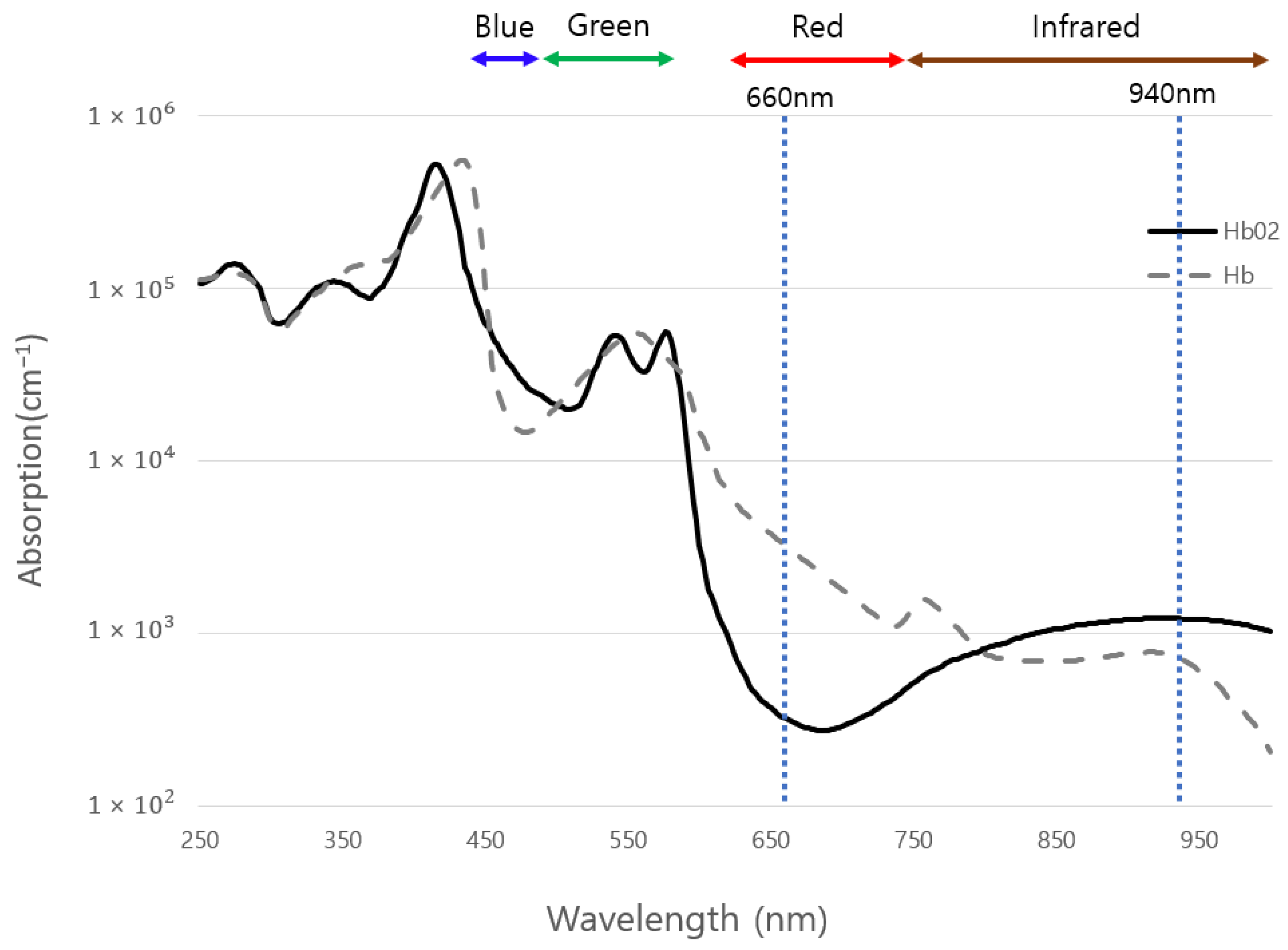
In general, non-contact oxygen saturation studies are based on the operating principle of a pulseoximeter. A pulseoximeter is based on the principles of the different absorptions of different light wavelengths by hemoglobin species. A pulseoximeter transmits infrared and red light to the finger. As shown in
Figure 1, hemoglobin without oxygen and hemoglobin with oxygen absorb infrared and red light differently. At this time, hemoglobin that is not bound to oxygen absorbs more infrared light, and hemoglobin that is bound to oxygen absorbs more red light.
The pulseoximeter measures and analyzes the amount of light absorbed by the sensor. It determines the oxygen saturation in the blood by calculating the difference in absorption for infrared and red light [
9]. In measuring oxygen saturation, the alternating current (AC) and direct current (DC) components form an important part of the principle of measurement. By measuring the transmitted light hundreds of times per second, the pulseoximeter can distinguish between the AC component, which is a variable pulsating component of arterial blood, and the DC component, which is an unchanging static component of a signal consisting of tissue, venous blood, and non-pulse arterial blood. The static component can then be removed from the signal so that the pulsating component, which is typically composed of 1% to 5% of the total signal, can be separated. As shown in Equation (1), dividing the AC level by the DC level at each wavelength also compensates for the change in the incident light intensity, which can remove other complex variables from the equation. Doing this at each wavelength reduces the main source of absorption in the arterial blood and separates the relative absorbance of oxygenated Hb. The ratio of the red signal (
/
) to the infrared signal (
/
) reflects a ratio similar to that of oxygenated Hb, which can be converted to oxygen saturation through Equation (2) [
10].
Reviewing existing studies summarized in
Section 2, the method of calculating the AC and DC components was also used in the non-contact oxygen saturation measurement. However, since IR wavelengths are not observed in RGB cameras, as shown in
Figure 1, a visible light wavelength band with light absorption characteristics similar to IR was used. However, unlike pulseoximetry, this method is highly sensitive to factors such as skin color and ambient lighting conditions. Therefore, the methods for calculating the AC and DC components are different in each existing paper, and this diversity can affect the accuracy and reliability of the results. In fact, existing studies have not been able to produce satisfactory results.
Therefore, in this study, the oxygen saturation was estimated using the signals obtained from the video as the input of the model without calculating the AC and DC components. Specifically, we separated the signals obtained from videos into 10 color spaces and predicted the oxygen saturation using a ResNet-based deep learning model. We investigated the feasibility of various color components, rather than specific wavelength color components, in reflecting the oxygen saturation values. Considering the time-consuming nature of accurately measuring the oxygen saturation, we diversified the model inputs into 10 s, 20 s, and 30 s intervals to compare performance. Additionally, we analyzed the color channels contributing to oxygen saturation prediction on a per-subject basis using SHAP (Shapley additive explanations).
2. Related Works
Recently, methods have been proposed to measure oxygen saturation non-invasively using facial or hand images. These methods utilize specialized cameras with filters capable of capturing specific wavelength bands [
11] or commonly available RGB cameras such as webcams or smartphone cameras. While specialized cameras can capture wavelength bands suitable for measuring oxygen saturation, they are not widely used. Therefore, there is a need for methods that can measure oxygen saturation using RGB cameras.
Previous studies that utilize RGB cameras for measuring oxygen saturation have primarily employed the ratio of ratios (RoRs) method. Tarassenko et al. [
12] and Rahman et al. [
13] estimated the AC and DC components for red and blue wavelengths from the facial region of the RGB image and calculated the RoRs to measure oxygen saturation. Sun et al. [
14] estimated the AC and DC components for red and green wavelengths from the dorsum of the hand region in the RGB image and calculated the RoRs to measure oxygen saturation.
Additionally, some methods go beyond using two wavelength bands and utilize all three channels of the RGB image. Wei et al. [
15] estimated the AC and DC components by using all three wavelength bands from the facial region of the RGB image, while Tian et al. [
16] estimated the AC and DC components by using all three wavelength bands from the palm region of the RGB image and calculated the RoRs to measure oxygen saturation.
Furthermore, methods that use convolutional neural networks (CNNs) to measure oxygen saturation have been proposed, which differ from previous regression-based methods. Akamatsu et al. [
17] calculated the AC and DC components using the red, green, and blue wavelengths from the facial region of the RGB image and fed the resulting spatiotemporal map into a CNN model to measure oxygen saturation.
Various papers have proposed methods using RGB cameras to measure oxygen saturation, with most considering the AC and DC components. However, the methods for estimating the AC and DC components from the photoplethysmography (PPG) signal, despite the clear relationship between RoRs and oxygen saturation, vary among the papers.
In the examined papers, Tarassenko et al. [
12] calculated the AC component as the average of the peaks and valleys in the PPG signal and the DC component as the mean of the PPG signal. Rahman et al. [
13] calculated the AC component as the standard deviation of the PPG signal and the DC component as the mean of the PPG signal. Sun et al. [
14] applied band-pass filtering with a bandwidth of 0.5–5 Hz to obtain the AC component and low-pass filtering with a cut-off frequency of 0.3 Hz to obtain the DC component. Wei et al. [
15] performed band-pass filtering with a bandwidth of 0.6–3 Hz to obtain the AC component and low-pass filtering with a cut-off frequency of 3 Hz to obtain the DC component. Tian et al. [
16] used an eighth-order Butterworth filter with a bandwidth of 0.1 Hz centered around the estimated heart rate to obtain the AC component as the average of the peaks and valleys in the filtered signal and a second-order low-pass Butterworth filter with a cut-off frequency of 0.1 Hz to obtain the DC component as the median of the filtered signal. Akamatsu et al. [
17] applied band-pass filtering with a bandwidth of 0.75–2.5 Hz to obtain the AC component and low-pass filtering with a cut-off frequency of 0.3 Hz to obtain the DC component.
While extracting the AC and DC components is essential in the principle of estimating oxygen saturation, the performance of predicting oxygen saturation varies greatly depending on how these components are extracted [
16]. Therefore, in this paper, we proposed a method for estimating oxygen saturation using RGB cameras without arbitrarily extracting the AC and DC components, utilizing the time-series data obtained from RGB images.
Table 1 shows a summary of the related works.
3. Method
In this study, oxygen saturation was calculated using acquired images. To do this, the segment corresponding to the skin area in the image was extracted by using RGB values, and the RGB signals in the skin area were then obtained. Afterwards, the RGB signal was converted to YCrCgCb and the HSV color space, and then these signals were used to generate 10-dimensional feature data. Afterward, the oxygen saturation was calculated using a ResNet-based CNN model.
Figure 2 shows the overall process.
3.1. Dataset
In this study, an experiment was conducted by controlling the factors that could affect the oxygen saturation prediction, such as race, distance, and lighting. A total of 14 Korean participants (eight males and six females) between the ages of 24 and 32 took part in the experiment.
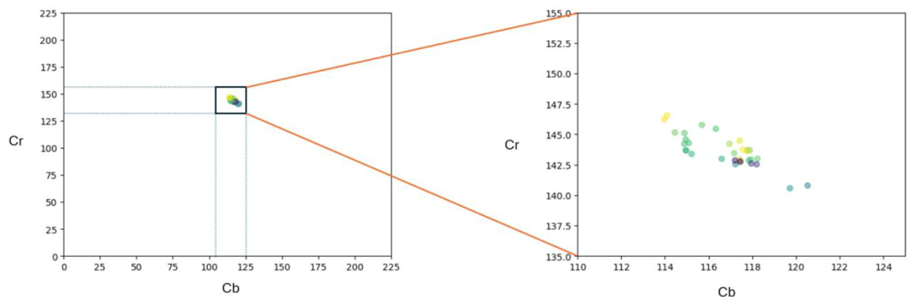
Table 2 shows the demographic characteristics and the average values of the Cg and Cb color channels of the subjects.
Figure 3 displays the distribution of skin colors for all the data. Since the study was limited to Koreans, the dots were clustered in one area. During the data collection, the participants were instructed to sit comfortably and minimize movement as much as possible. Additionally, they were asked to hold their breath to lower their oxygen saturation levels, and if they experienced discomfort, they were instructed to resume breathing. Each experiment lasted for 5 min and 30 s, during which breath-holding was repeated three times. Each participant took part in the experiment twice.
The experiment was conducted in an indoor environment. To acquire the facial images, a conventional RGB camera (Logitech C920e) [
18] was used.
Figure 4 presents a comparison of the signals obtained from the Logitech C920e webcam, iPhone 14, and Galaxy Z Flip4. Since smartphones undergo their own color correction and other adjustments, it can be difficult to accurately assess color changes. For this reason, in this study, only the webcam (Logitech C920e) was used in the experiments to obtain more accurate and reliable results. To enable the participants to comfortably sit in the chair and participate in the experiment, the camera was placed 60 cm away from the participants and captured facial images at a speed of 30 frames per second with a resolution of 640 × 480 pixels. Simultaneously, to measure the oxygen saturation levels, the participants’ fingers were attached to a CMS-50E pulseoximeter [
19]. This device was synchronized with the recorded images using timestamps. Prior to the experiment, consent was obtained from all the participants. The averages of the Cg and Cb color channels in
Table 2 were calculated as the mean values of the two experimental datapoints for each participant.
3.2. Data Preprocessing
The facial images obtained through the camera contained not only the face but also the clothing and background. To isolate only the face, a single-shot multiple detector (SSD) face detector was used to detect the faces in the images. However, the detected face regions still included the eyebrows, hair, and other elements. To remove these unwanted components, the RGB color space of the image was converted to the YCbCr color space, and only the skin region was selected. The selected range for the skin region was 0 ≤ Y ≤ 235, 77 ≤ Cb ≤ 127 and 133 ≤ Cr ≤ 173 [
20].
After this process, the selected skin region was in the RGB color space. In this paper, the selected skin region of interest (ROI) used a time series of 10 channels (R, G, B, Y, Cr, Cg, Cb, H, S, and V) as the data. Therefore, the RGB signals were transformed into the YCrCgCb and HSV signals. To do this, the average values of R, G, and B per frame were calculated within the selected ROI. These values were then normalized to the range from 0 to 1 by dividing them by the maximum pixel value of 255. We denoted the normalized R, G, and B signals as R′, G′, and B′, respectively. Using Equations (3)–(6) [
21] and Equations (7)–(12) [
22], the RGB signals could be transformed into the YCrCgCb and HSV signals, respectively.
Using the RGB signals and the transformed YCrCgCb and HSV signals, a dataset of size N × 10 was generated, where N represents the number of frames in the video. In this paper, considering that it takes a minimum of 30 s to successfully measure oxygen saturation [
23], signals from 10, 20, and 30 s were used, resulting in dataset lengths of 300, 600, and 900, respectively.
As mentioned in
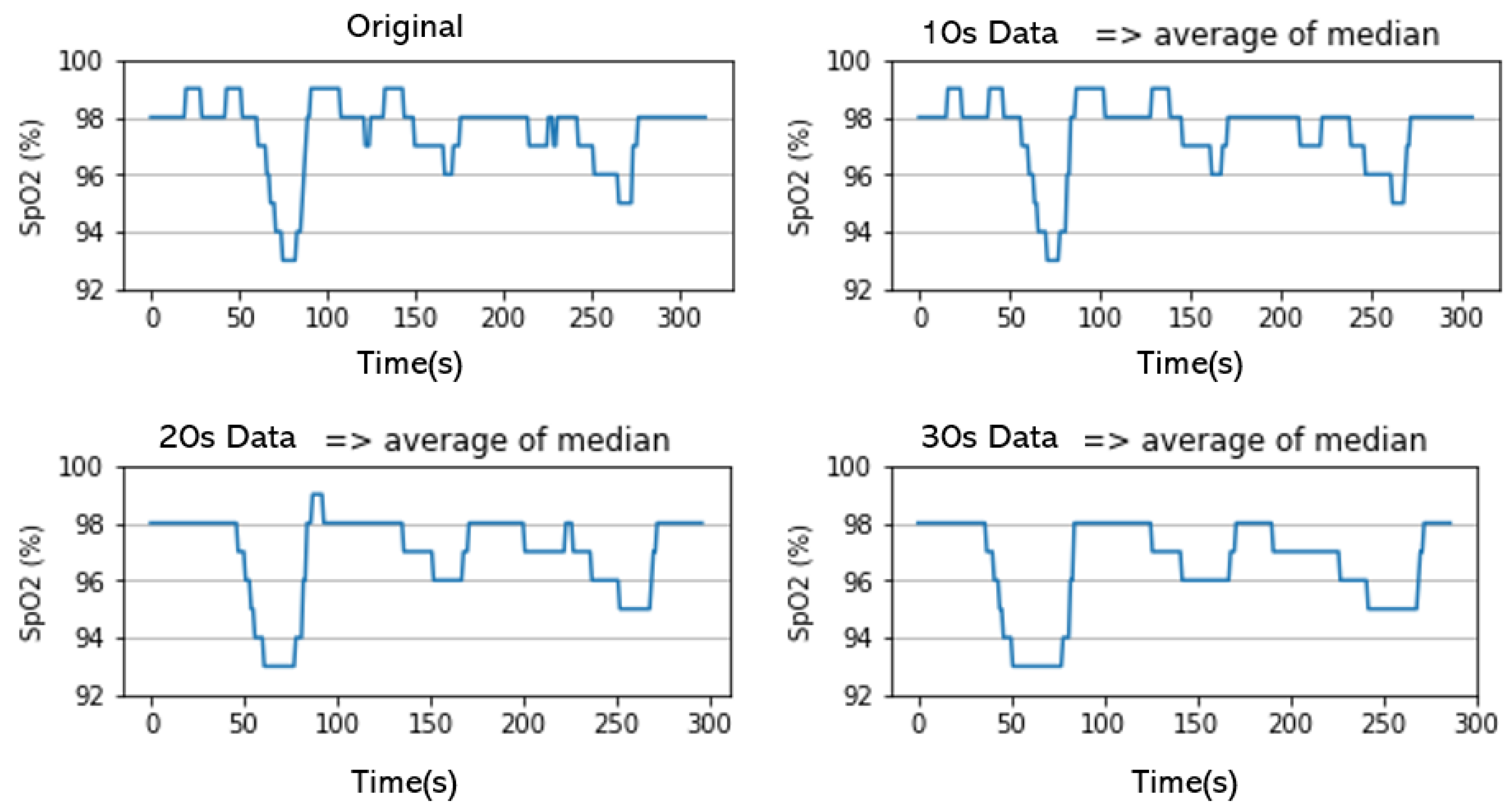
Section 3.1, the oxygen saturation values were measured at a sampling rate of 1 Hz during image acquisition. Therefore, the length of the generated data needed to be adjusted accordingly. For example, when using the signals from a 10-second period, only one of the 10 oxygen saturation values measured during that time should be selected. In this paper, to best represent the decreasing trend of oxygen saturation while preserving the original values, the average of the median values was used. To calculate this, the
n oxygen saturation values (in this case,
n = 10, 20, 30) were first sorted, and then the average value of the oxygen saturation values corresponding to the third interval, divided into five intervals, was taken.
Figure 5 shows the resulting signals when the original signal and the oxygen saturation values for 10, 20, and 30 s were calculated using the average of the median values for one of the participants.
3.3. Model Training Method
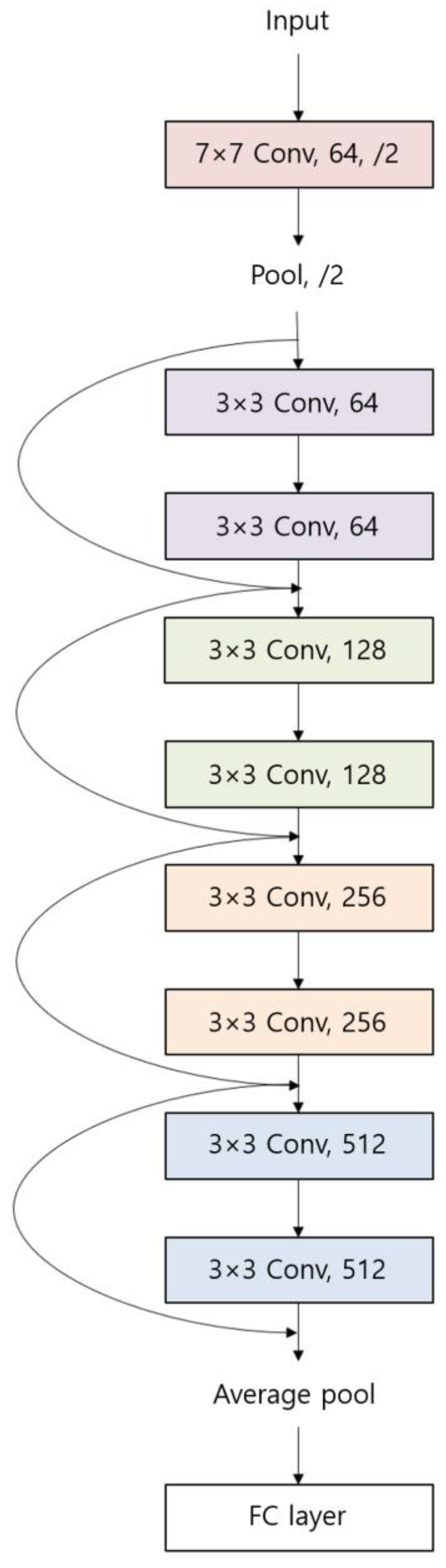
In this paper, a CNN model based on ResNet [
24] was created to measure oxygen saturation using the N × 10 dataset generated in
Section 3.2.
Figure 6 illustrates the structure of the model developed in this paper for measuring oxygen saturation. Similar to ResNet, skip connections were used in this model to combine the input data with the output at each layer and pass it to the next layer.
The model training was conducted three times, each time using input data of size 300 × 10, 600 × 10, and 900 × 10. Two videos obtained from each participant were used, with one video used for model training and the other for testing. The loss was updated using the mean square error, and the Adam optimizer [
25] was employed as the optimization algorithm. The batch size was set to 32, and the maximum number of epochs was set to 4000 for training. For testing, the model from the epoch with the lowest loss was utilized, and sliding windows of 1 s were used to obtain continuous outputs.
In the initial layers of ResNet, low-level features are primarily extracted, which mainly encompass basic information related to changes in each color space. At this stage, the model can learn information such as the average color variations and relationships between the colors. In the later stages of the model, based on the low-level features extracted in the initial layers, more complex patterns are recognized, and crucial information related to oxygen saturation is derived. By integrating various features across channels and time frames, such as temporal change analysis and a combination of high-level features, the model learns complex patterns that accurately predict oxygen saturation. This is crucial for the model to draw meaningful conclusions about oxygen saturation from changes in the color space. In conclusion, while the initial layers of ResNet extract basic information, such as the average color variations in each color space, the later layers combine and analyze this information to understand and predict more complex patterns related to oxygen saturation. In this study, half of the 28 videos acquired from the 14 participants were used to train the model, while the remaining videos were used for testing.
4. Results
To quantitatively evaluate the performance of the trained model in predicting oxygen saturation, we used the Pearson correlation coefficient, mean absolute error, and root mean square error. The Pearson correlation coefficient is one of the methods used to measure the linear correlation between two variables, indicating a strong correlation between the variables when the absolute value is close to 1. The mean absolute error represents the average error between the predicted and actual values, and smaller values indicate better predictive performance of the model. The root mean square error represents the square root of the average of the squared differences between the predicted and actual values, indicating the standard deviation of the prediction errors. Smaller values suggest better predictive performance, and like the mean absolute error, it is used for model evaluation and comparison. However, the root mean square error is more sensitive to larger errors, as its values increase with larger errors, making it more sensitive for evaluating model performance compared to the mean absolute error.
4.1. Results by Subject
The experimental results are as follows:
Figure 7,
Figure 8 and
Figure 9 depict a comparison between the oxygen saturation estimated using the model trained with data from 10, 20, and 30 s, respectively, and the oxygen saturation measured using the contact-based sensor. The complete results for all participants are summarized in
Table 3,
Table 4 and
Table 5.
The results indicate that the trained model did not perform well in predicting oxygen saturation compared to previous studies. However, it is important to note that previous studies on the non-contact estimation of oxygen saturation evaluated the results by averaging the individual training and testing results for each participant. Taking this into consideration, our study also conducted training and testing on a participant-specific basis.
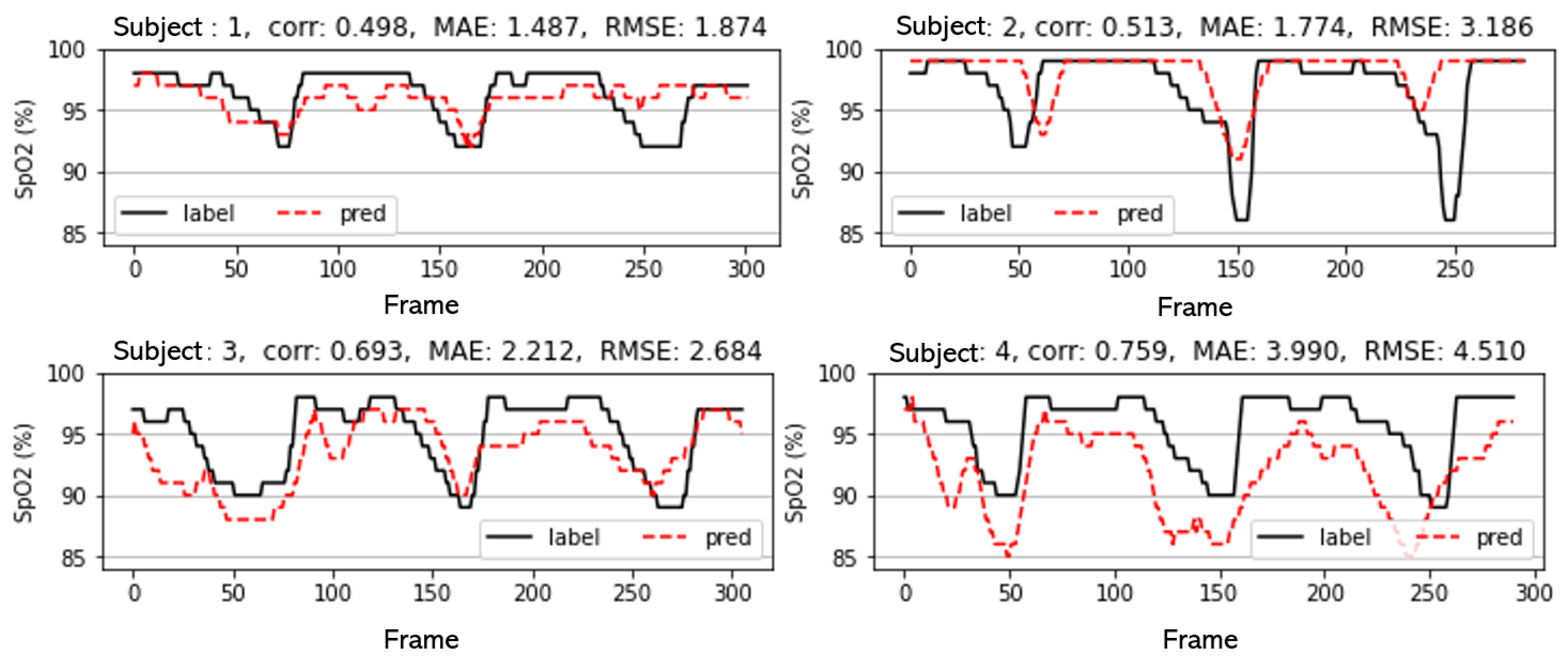
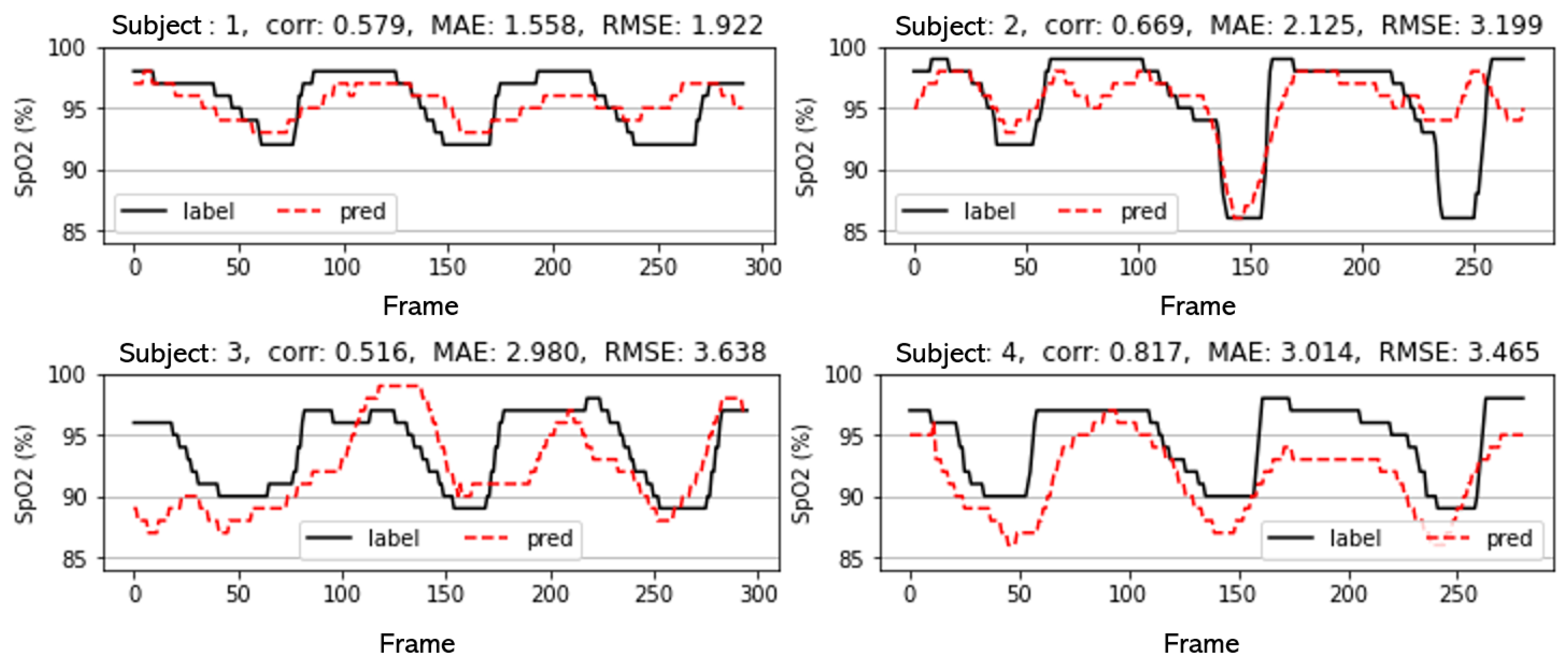
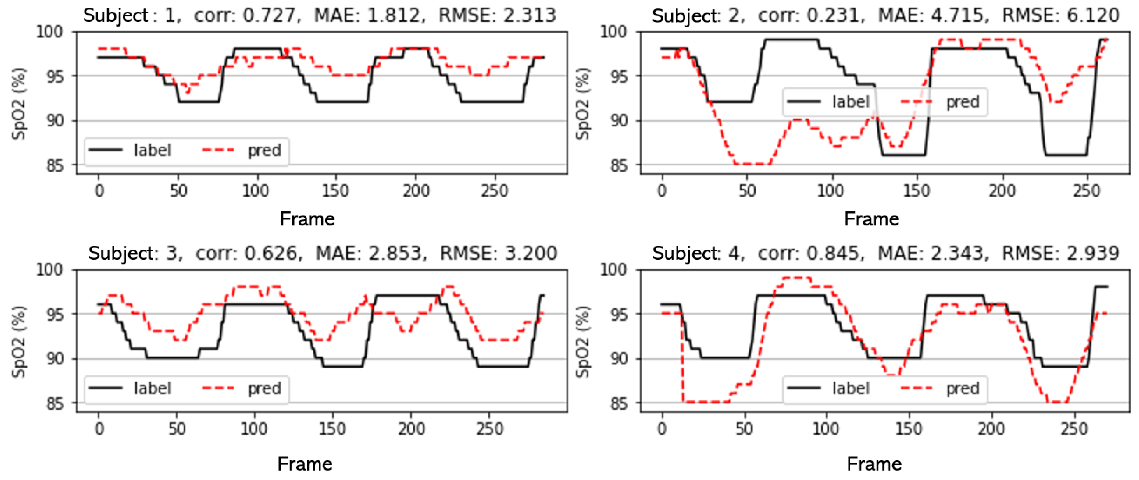
Figure 10,
Figure 11 and
Figure 12 show selected graphs comparing the oxygen saturation estimated using the model trained with data from 10, 20, and 30 s, respectively, with the oxygen saturation measured using the contact-based sensor. The complete results for all participants are summarized in
Table 6,
Table 7 and
Table 8. The intraclass correlation coefficient (ICC), which measures the agreement between two evaluations, ranged between 0 and 1.
Upon examining the results, it can be observed that the individual models performed either better or comparably to previous studies, and there was a significant difference in exactness compared to the ensemble model. In
Section 4.2, the reasons for the discrepancies in the output values between the individual and ensemble models are analyzed.
4.2. Feature Analysis
In order to analyze the features used by the trained model for prediction based on the observed differences in the output values between the individual and ensemble models in
Section 4.1, SHAP (Shapley additive explanations) was employed [
26]. SHAP is based on the concept of Shapley values, which is derived from cooperative game theory. Shapley values measure the worth of each player in a cooperative game. When applied to evaluating feature importance in machine learning models, SHAP values provide insights into the impact of features on model predictions.
The range of SHAP values varies depending on the characteristics of the features and the model’s structure. The absolute magnitude of a SHAP value represents the contribution of each feature, indicating the extent to which it influences the model’s prediction. A larger SHAP value indicates a greater impact of the corresponding feature on the model’s prediction.
When calculating the SHAP values for each feature, all combinations of features are considered to evaluate the model’s predictions. In other words, the difference between the model’s predictions when a feature is excluded and the original predictions is computed, and this difference represents the importance (SHAP value) of that feature.
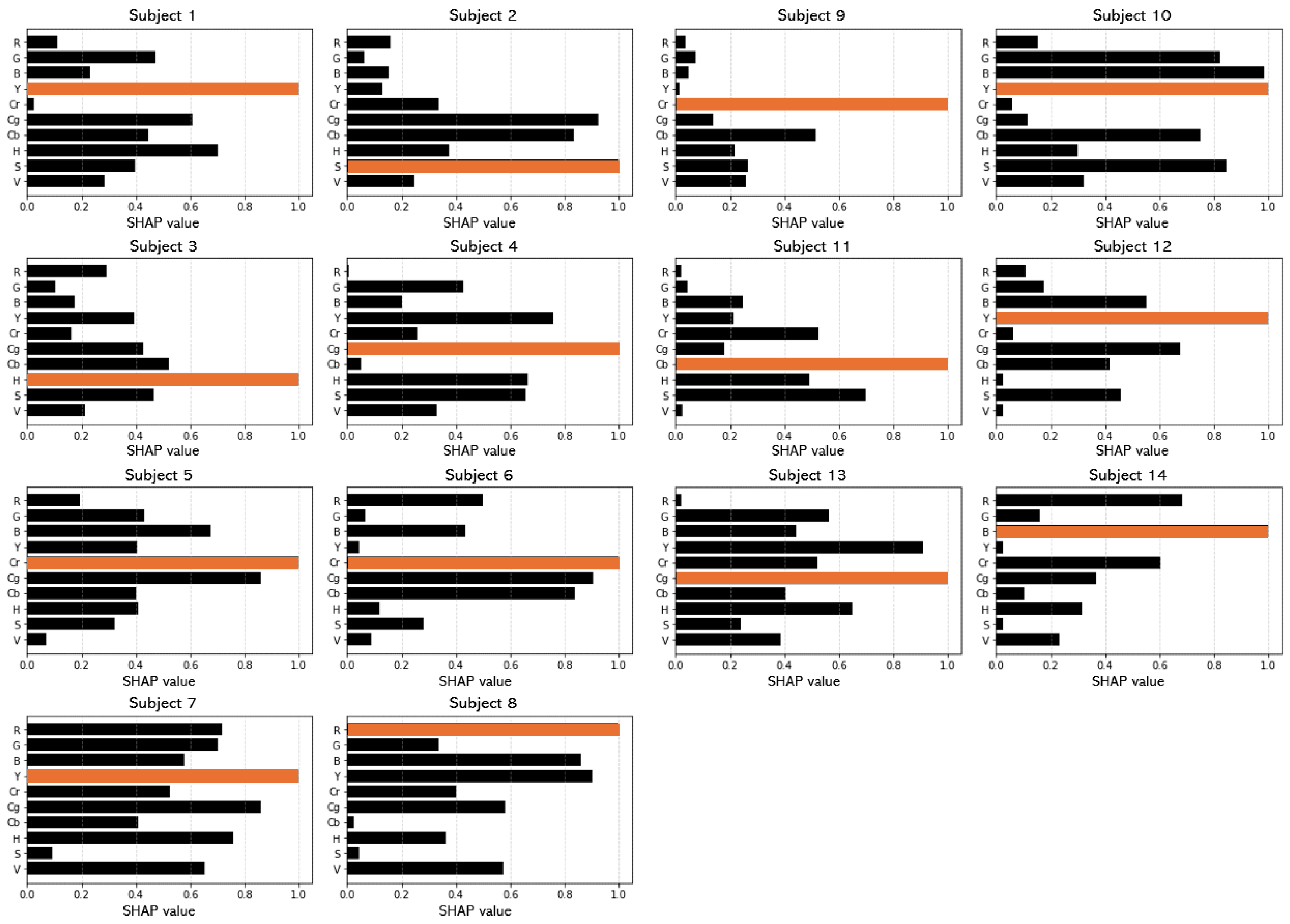
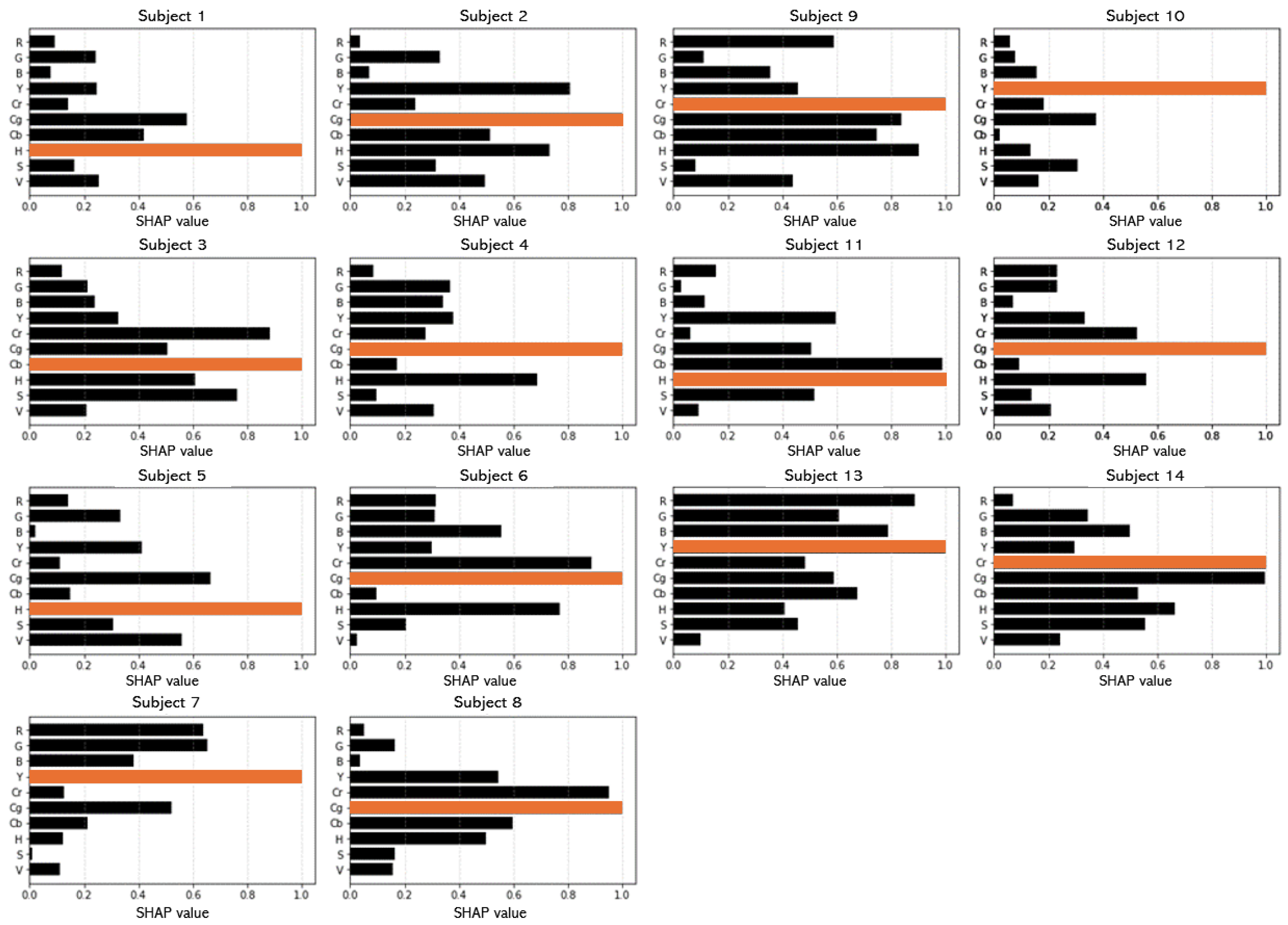
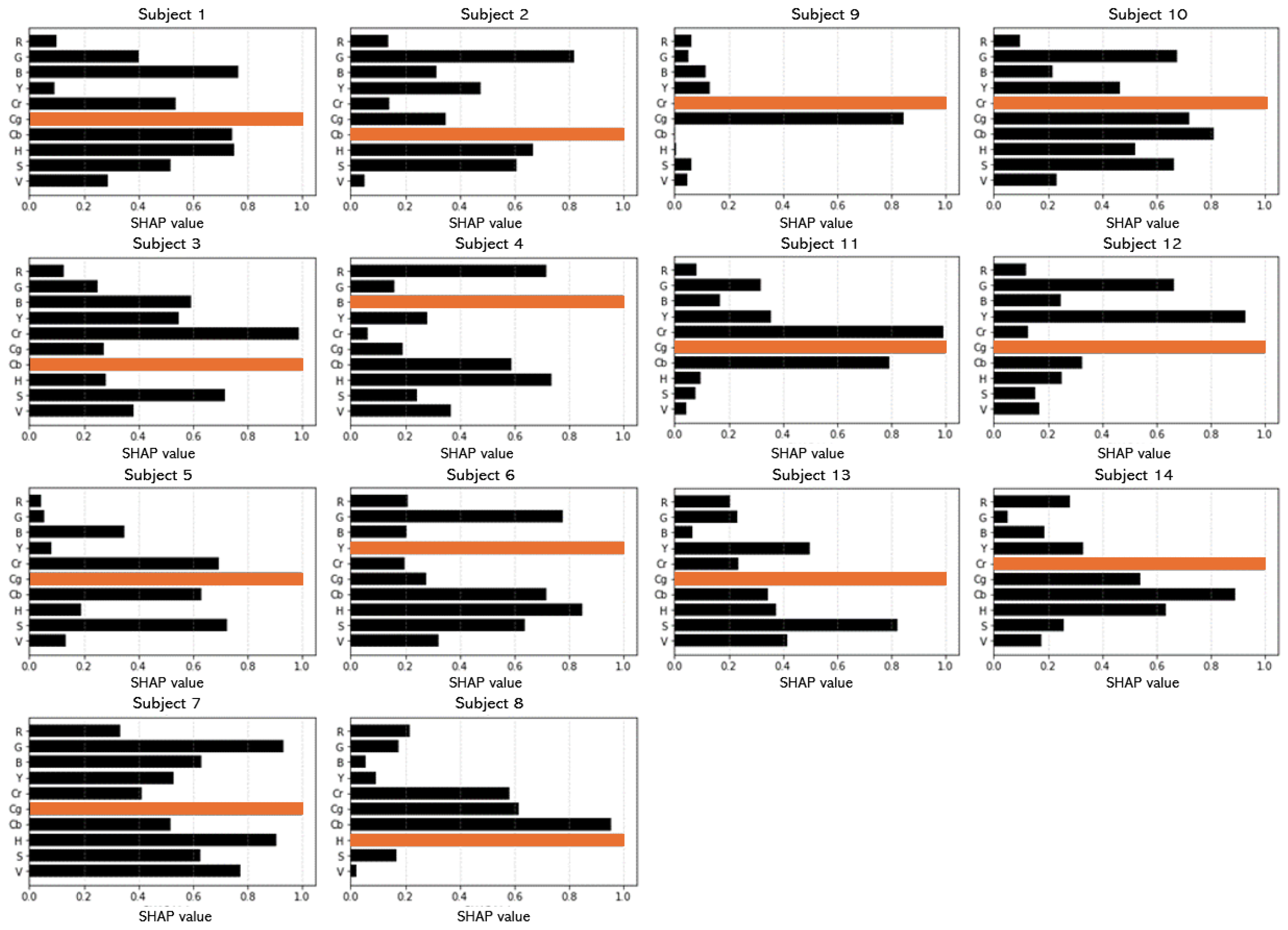
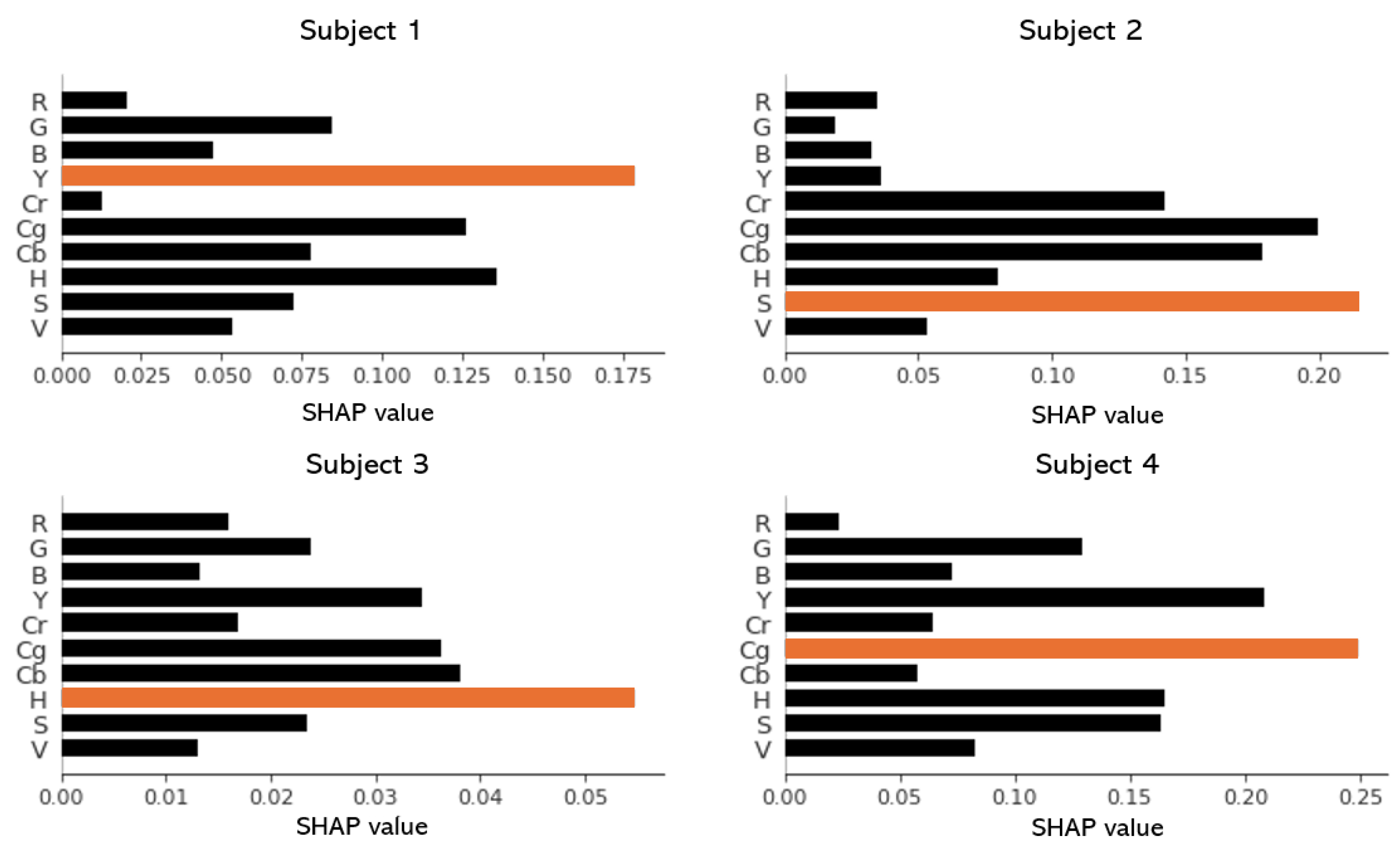
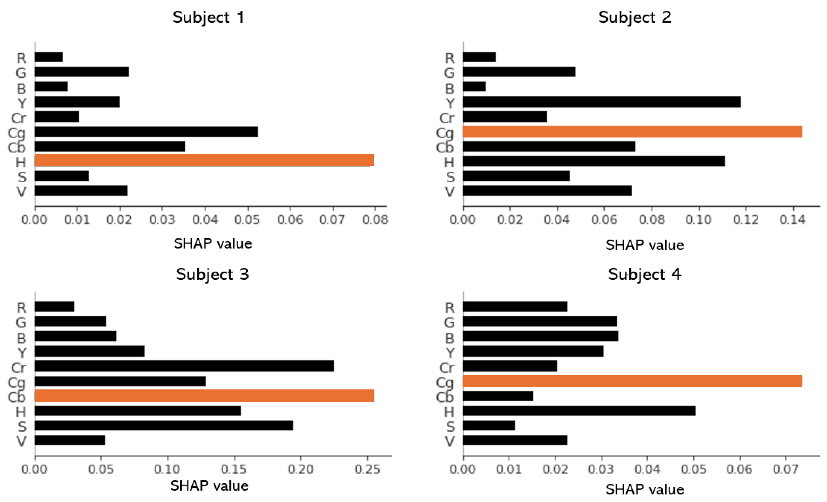
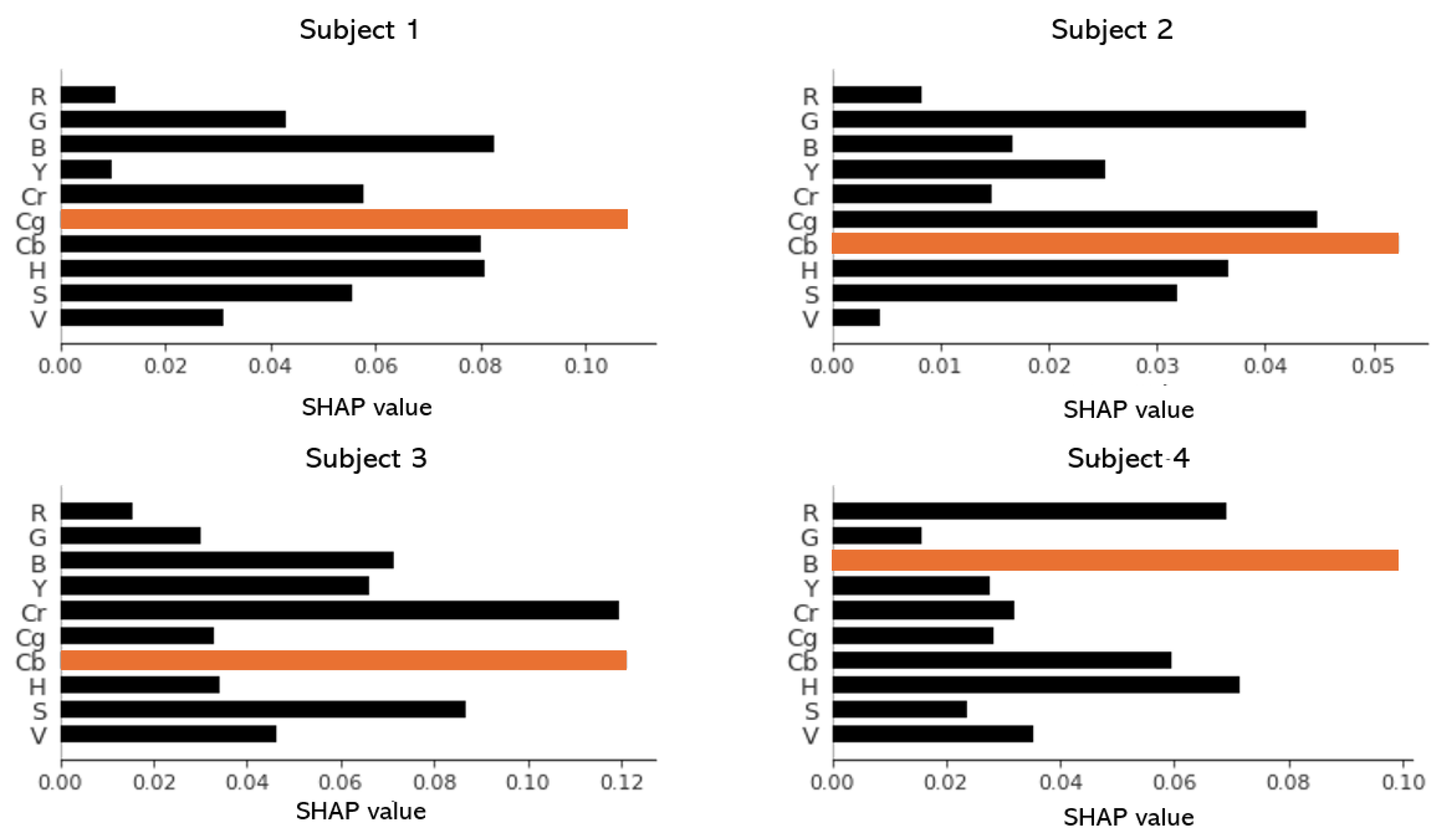
Figure 13,
Figure 14 and
Figure 15 depict the SHAP values and feature contributions for the individual models trained and tested on the data used in
Figure 10,
Figure 11 and
Figure 12. These visualizations were used to confirm whether the features with dominant contributions significantly impacted each individual participant.
Figure 13,
Figure 14 and
Figure 15 indicate significant variations in the importance of the features among different subjects. Furthermore, since these graphs demonstrate the contribution to the data used for training, it is confirmed whether the feature with the predominant contribution was important to each subject by confirming the contribution to the data used in testing.
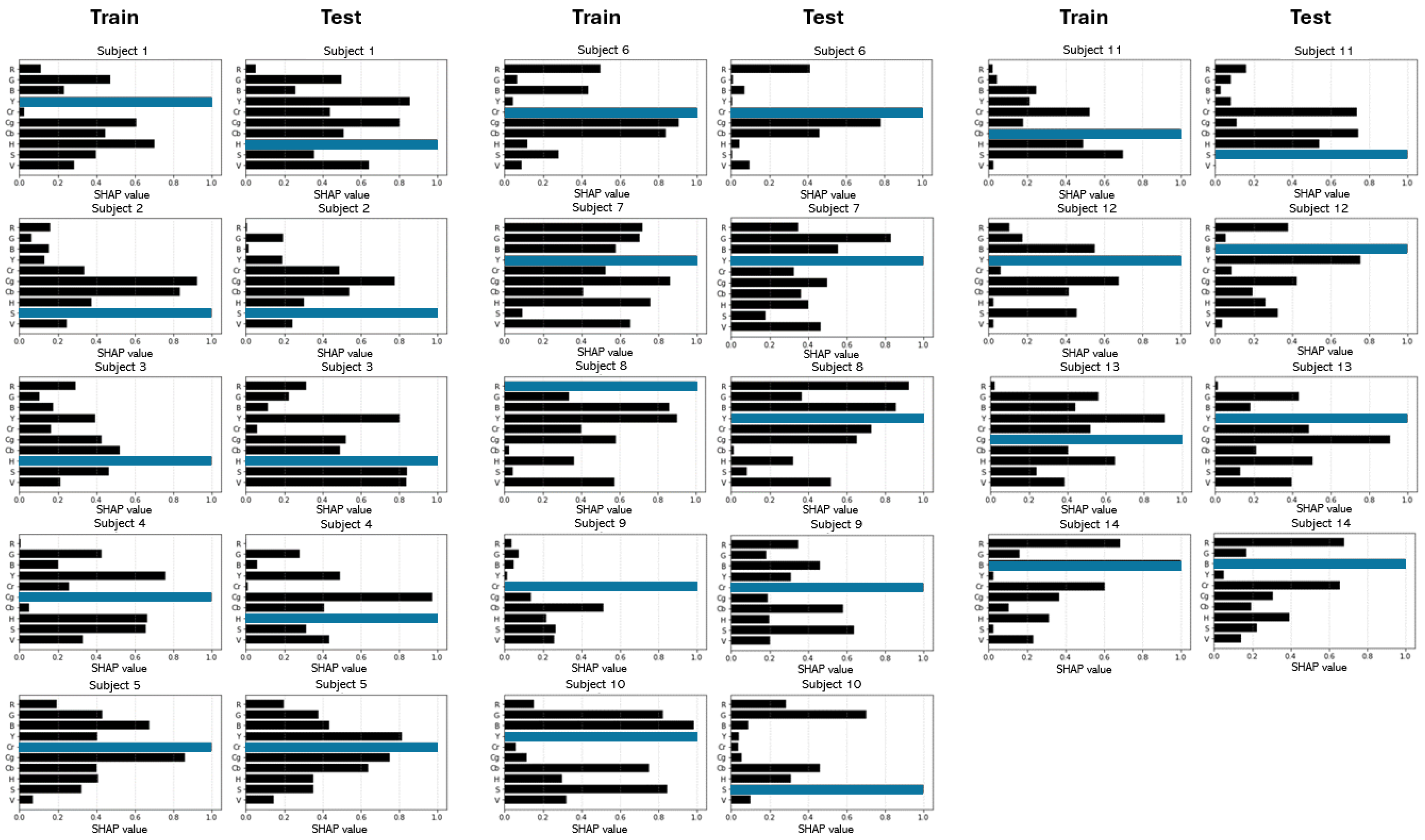
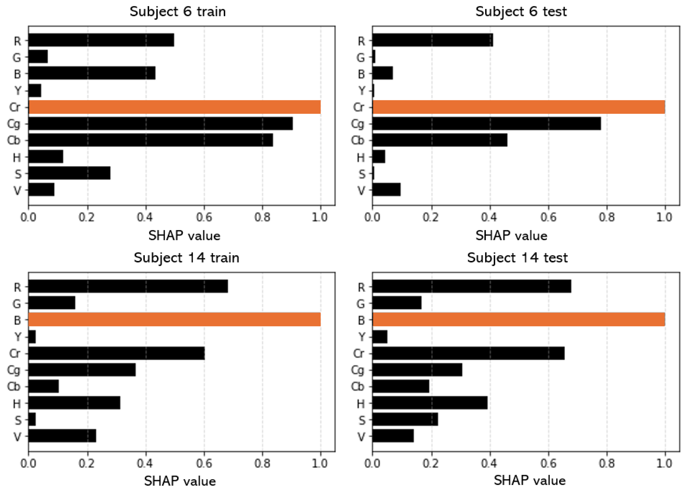
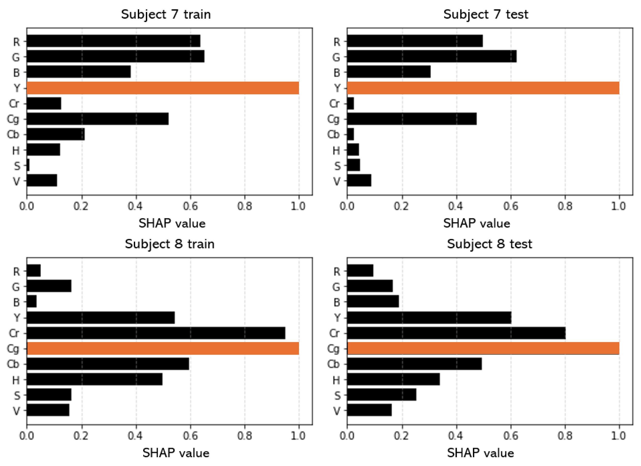
Figure 16,
Figure 17 and
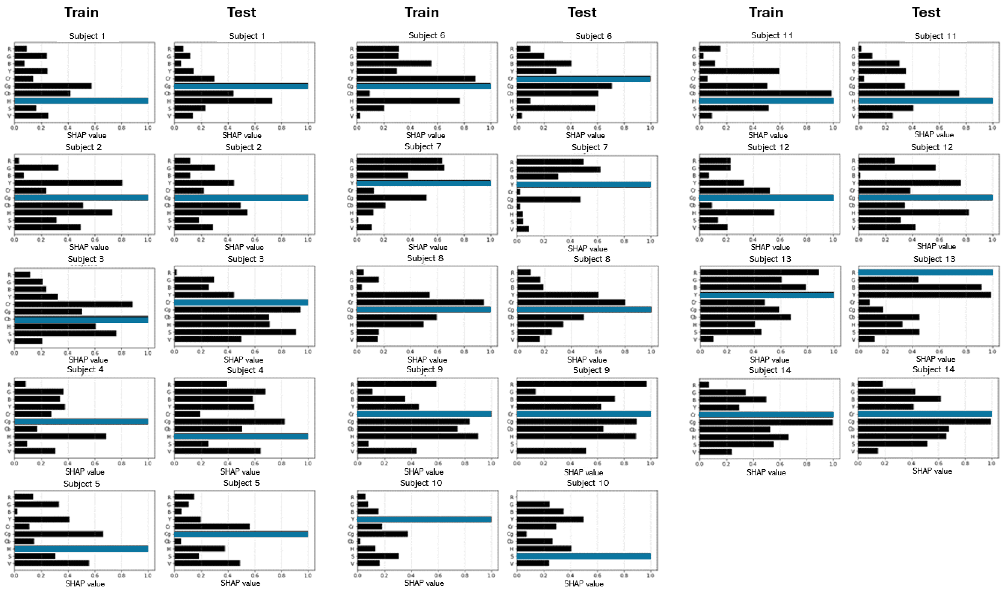
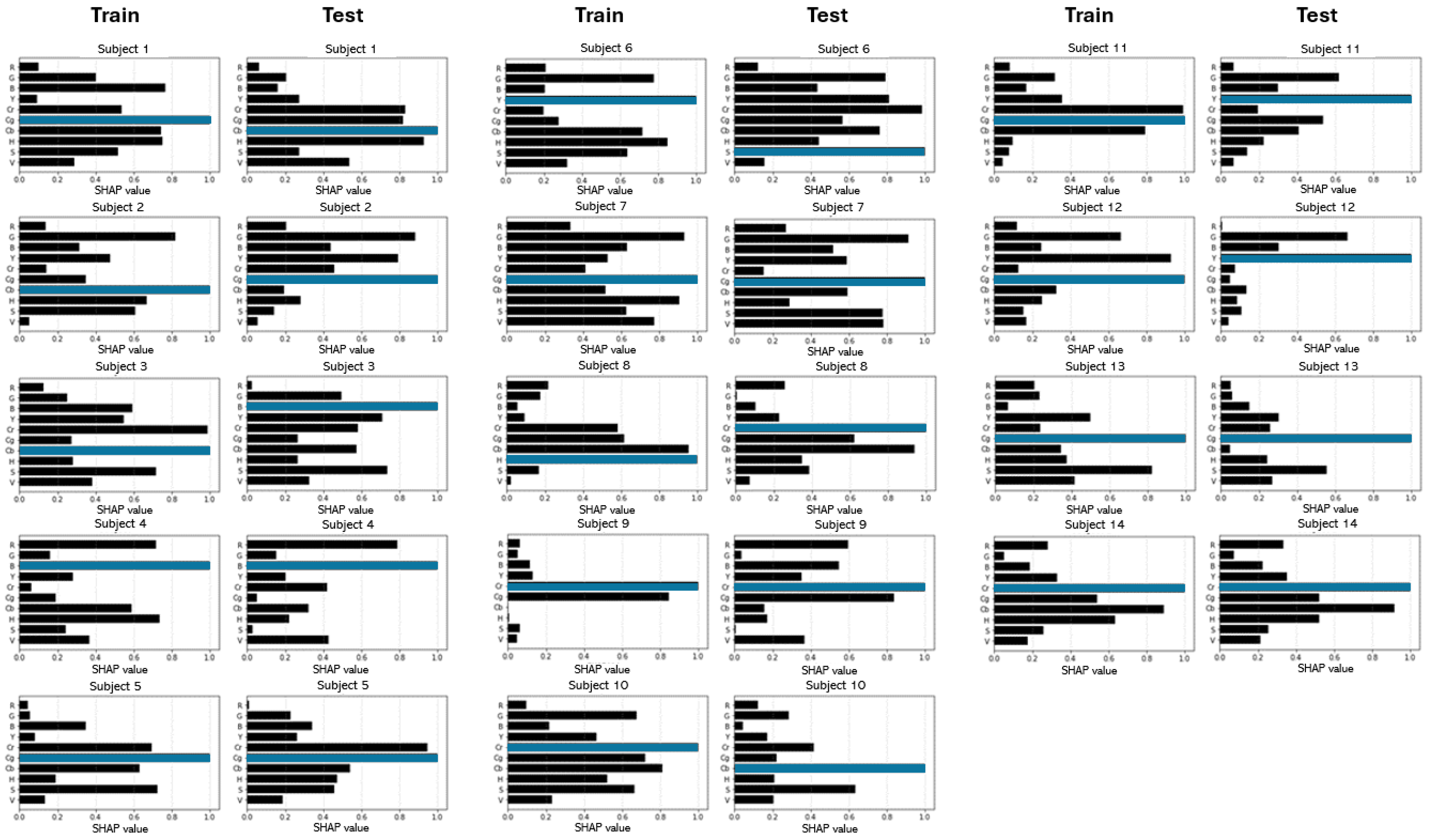
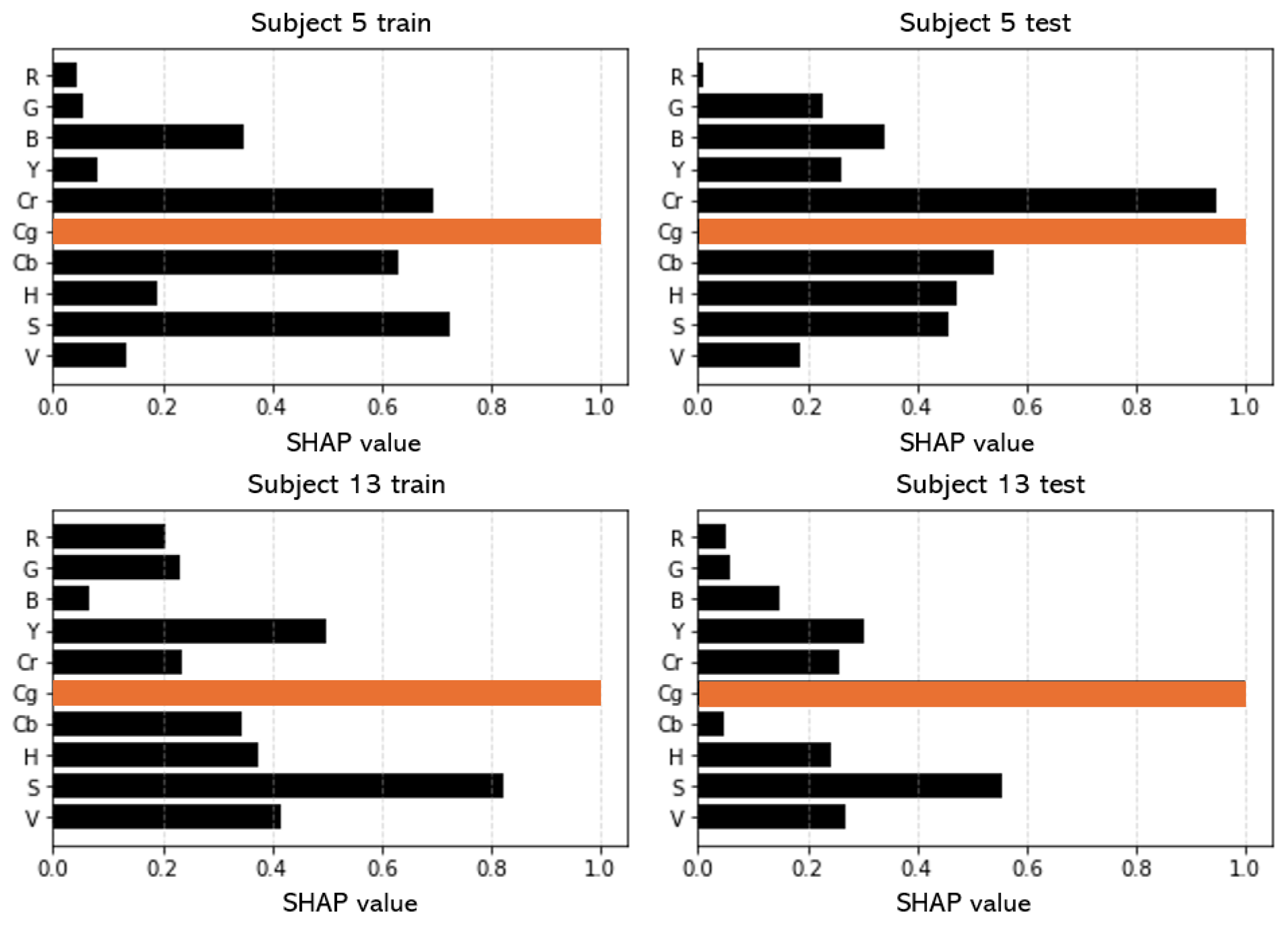
Figure 18 show the results, displaying the SHAP values for models trained on input data for 10 s, 20 s, and 30 s.
For each subject in
Figure 16, the Cr and B channels contributed the most. In
Figure 17, the Y and Cg channels were the primary contributors for each respective subject, and in
Figure 18, the Cg channel had the largest contribution. When examining individual models for all subjects, it became evident that most subjects had the same predominant features contributing to both the training and testing data. Considering not only the differences in feature importance but also the fact that the features contributing the most to the predictions vary from person to person, this supports the idea that personalized models perform better in predicting oxygen saturation than a unified model. Additionally, it suggests that in future research aimed at improving the exactness of oxygen saturation prediction, it may be necessary to individually select appropriate color channels for each subject rather than relying solely on the conventional approach of using specific color channels. Feature analysis graphs for all subjects are included in
Appendix A.
5. Discussion
This paper proposed a method for estimating oxygen saturation using convolutional neural networks and images acquired with an RGB camera. Because the AC and DC components, which are essentially calculated in the measurement of oxygen saturation, can vary sensitively depending on the calculation method, the time-series data of the image was directly utilized. Furthermore, to account for the significant time required for successful oxygen saturation measurement, experiments were conducted with varying input times.
Table 9 summarizes the oxygen saturation prediction results according to the input data lengths.
First, we trained a unified model using half of the images acquired from the subjects and conducted tests. The results were as follows: when using 10 s of data, the Pearson correlation coefficient was calculated as 0.414, with the MAE (mean absolute error) and RMSE (root mean square error) calculated as 2.592% and 3.108%, respectively. When using 20 s of data, the Pearson correlation coefficient was calculated as 0.473, with the MAE and RMSE calculated as 3.869% and 4.797%, respectively. When using 30 s of data, the Pearson correlation coefficient was calculated as 0.475, with the MAE and RMSE calculated as 3.025% and 3.547%, respectively. This can be considered as not accurately predicting oxygen saturation when compared to previous research. However, studies that measured oxygen saturation non-invasively and individually trained and tested for each subject generally. Therefore, in this study, similar to previous research, we conducted training and testing for each subject separately. As a result, for a 10-second input, the Pearson correlation coefficient was calculated as 0.570, with an MAE of 1.755% and RMSE of 2.284%, with an ICC (intraclass correlation coefficient) of 0.574. For a 20-second input, the Pearson correlation coefficient was calculated as 0.630, with an MAE of 1.720% and RMSE of 2.219%, with an ICC of 0.681. For a 30-second input, the Pearson correlation coefficient was calculated as 0.663, with an MAE of 2.142% and RMSE of 2.612%, with an ICC of 0.646. In comparison to the previous studies [
15,
17] that estimated oxygen saturation from the facial region of interest (ROI), their average correlation coefficients were 0.68 and 0.49, respectively, indicating that these prior studies performed well in predicting oxygen saturation. Furthermore, the method proposed in this paper is more efficient as it utilizes the signals obtained from images without the need to calculate additional AC and DC components.
In this study, we investigated the factors influencing oxygen saturation estimation by controlling various variables such as illumination, distance, and skin tone through SHAP (Shapley additive explanations) value analysis. Particularly, the analysis utilizing the SHAP values revealed significant variations in the feature importance contributions across different subjects when the trained model predicted oxygen saturation. This finding suggests that there may be diverse sets of features that exert the greatest influence on predictions for each individual. Therefore, to improve the accuracy of oxygen saturation predictions, it may be necessary to move beyond the conventional approach of using specific color channels and instead consider employing different color channels for each subject.
However, this study did not utilize a more diverse dataset encompassing various demographics such as gender, age, and skin tone. This limitation could impact the generalizability of the research findings. For instance, certain gender, age, or skin tone groups may have different color channels that affect oxygen saturation. Future research should analyze the color channels contributing to oxygen saturation prediction in greater detail by utilizing more diverse datasets, thereby enhancing our understanding of the influences of features and improving the predictive power of the model across different environments.
Furthermore, the database used in this study only included oxygen saturation values ranging from 85% to 100%, obtained by instructing participants to hold their breath. Therefore, models trained to predict oxygen saturation using this database may exhibit a tendency to predict lower oxygen saturation values than those used in training. To address this limitation, it is necessary to employ more diverse databases reflecting a wider range of oxygen saturation values. Considering that in the future, the International Organization for Standardization (ISO) will verify the accuracy of pulseoximeters through hypoxia-induced clinical trials that change oxygen saturation by 70 to 100%, the data needs to diversify the range of oxygen saturation changes. This will involve utilizing datasets with a more varied range of oxygen saturation changes for predicting oxygen saturation.
Therefore, future research plans involve conducting studies to predict oxygen saturation using more diverse datasets that consider gender, age, skin color, and varied ranges of oxygen. This will involve analyzing the color channels contributing to oxygen saturation prediction and diversifying prediction models by grouping individuals with similar contributions from each color channel without creating individualized models.
Author Contributions
Conceptualization, E.C.L.; methodology, H.A.S. and C.L.S.; data collection, H.A.S.; software, H.A.S. and C.L.S.; validation, H.A.S.; formal analysis, H.A.S. and C.L.S.; investigation, H.A.S. and C.L.S.; writing—original draft preparation, H.A.S. and C.L.S.; writing—review and editing, E.C.L.; visualization, H.A.S.; supervision, E.C.L.; project administration, E.C.L. All authors have read and agreed to the published version of the manuscript.
Funding
This paper was supported by the Field-oriented Technology Development Project for Customs Administration through the National Research Foundation of Korea (NRF) funded by the Ministry of Science and ICT and Korea Customs Service (2022M3I1A1095155).
Institutional Review Board Statement
Based on the 13-1-3 of the Enforcement Regulations of the Act on Bioethics and Safety of the Republic of Korea, ethical review and approval were waived (IRB-SMU-C-2023-1-008) for this study by Sangmyung University Institutional Review Board, because this study uses only simple contact measuring equipment or observation equipment that does not follow physical changes.
Informed Consent Statement
Informed consent was obtained from all subjects involved in the study.
Data Availability Statement
The original contributions presented in the study are included in the article, further inquiries can be directed to the corresponding author.
Conflicts of Interest
The authors declare no conflict of interest.
Appendix A
Figure A1.
SHAP values of the personalized model used in
Figure 10 (all subjects). The
x-axis represents the features and the
y-axis shows the contributions according to the features. Among them, the orange bar is the feature with the greatest contribution.
Figure A1.
SHAP values of the personalized model used in
Figure 10 (all subjects). The
x-axis represents the features and the
y-axis shows the contributions according to the features. Among them, the orange bar is the feature with the greatest contribution.
Figure A2.
SHAP values of the personalized model used in
Figure 11 (all subjects).
Figure A2.
SHAP values of the personalized model used in
Figure 11 (all subjects).
Figure A3.
SHAP values of the personalized model used in
Figure 12 (all subjects).
Figure A3.
SHAP values of the personalized model used in
Figure 12 (all subjects).
Figure A4.
SHAP values for the training and testing data of a model trained with 10 s of signals as the input data (all subjects).
Figure A4.
SHAP values for the training and testing data of a model trained with 10 s of signals as the input data (all subjects).
Figure A5.
SHAP values for the training and testing data of a model trained with 20 s of signals as the input data (all subjects).
Figure A5.
SHAP values for the training and testing data of a model trained with 20 s of signals as the input data (all subjects).
Figure A6.
SHAP values for the training and testing data of a model trained with 30 s of signals as the input data (all subjects).
Figure A6.
SHAP values for the training and testing data of a model trained with 30 s of signals as the input data (all subjects).
References
- Lewis, C.A.; Fergusson, W.; Eaton, T.; Zeng, I.; Kolbe, J. Isolated nocturnal desaturation in COPD: Prevalence and impact on quality of life and sleep. Thorax 2009, 64, 133–138. [Google Scholar] [CrossRef] [PubMed]
- American Academy of Sleep Medicine Task Force. Sleep-related breathing disorders in adults: Recommendations for syndrome definition and measurement techniques in clinical research. The Report of an American Academy of Sleep Medicine Task Force. Sleep 1999, 22, 667. [Google Scholar] [CrossRef]
- Starr, N.; Rebollo, D.; Asemu, Y.M.; Akalu, L.; Mohammed, H.A.; Menchamo, M.W.; Melese, E.; Bitew, S.; Wilson, I.; Tadesse, M.; et al. Pulse oximetry in low-resource settings during the COVID-19 pandemic. Lancet Glob. Health 2020, 8, e1121–e1122. [Google Scholar] [CrossRef] [PubMed]
- Severinghaus, J.W.; Honda, Y. History of blood gas analysis. VII. Pulse oximetry. J. Clin. Monit. 1987, 3, 135–138. [Google Scholar] [CrossRef] [PubMed]
- DeMeulenaere, S. Pulse oximetry: Uses and limitations. J. Nurse Pract. 2007, 3, 312–317. [Google Scholar] [CrossRef]
- Cheng, J.C.; Pan, T.S.; Hsiao, W.C.; Lin, W.H.; Liu, Y.L.; Su, T.J.; Wang, S.M. Using Contactless Facial Image Recognition Technology to Detect Blood Oxygen Saturation. Bioengineering 2023, 10, 524. [Google Scholar] [CrossRef]
- Sasaki, S.; Sugita, N.; Terai, T.; Yoshizawa, M. Non-Contact Measurement of Blood Oxygen Saturation Using Facial Video Without Reference Values. IEEE J. Transl. Eng. Health Med. 2023, 12, 76–83. [Google Scholar] [CrossRef]
- Prahl, S.A. Tabulated Molar Extinction Coefficient for Hemoglobin in Water. 1999. Available online: https://omlc.org/spectra/hemoglobin/summary.html (accessed on 18 January 2023).
- Chan, E.D.; Chan, M.M.; Chan, M.M. Pulse oximetry: Understanding its basic principles facilitates appreciation of its limitations. Respir. Med. 2013, 107, 789–799. [Google Scholar] [CrossRef] [PubMed]
- Sinex, J.E. Pulse oximetry: Principles and limitations. Am. J. Emerg. Med. 1999, 17, 59–66. [Google Scholar] [CrossRef] [PubMed]
- Humphreys, K.; Ward, T.; Markham, C. A CMOS camera-based pulse oximetry imaging system. In Proceedings of the 2005 IEEE Engineering in Medicine and Biology 27th Annual Conference, Shanghai, China, 17–18 January 2006. [Google Scholar]
- Tarassenko, L.; Villarroel, M.; Guazzi, A.; Jorge, J.; Clifton, D.A.; Pugh, C. Non-contact video-based vital sign monitoring using ambient light and auto-regressive models. Physiol. Meas. 2014, 35, 807–831. [Google Scholar] [CrossRef] [PubMed]
- Rahman, H.; Ahmed, M.U.; Begum, S. Non-contact physiological parameters extraction using facial video considering illumination, motion, movement and vibration. IEEE Trans. Biomed. Eng. 2019, 67, 88–98. [Google Scholar] [CrossRef] [PubMed]
- Sun, Z.; He, Q.; Li, Y.; Wang, W.; Wang, R.K. Robust non-contact peripheral oxygenation saturation measurement using smartphone-enabled imaging photoplethysmography. Biomed. Opt. Express 2021, 12, 1746–1760. [Google Scholar] [CrossRef] [PubMed]
- Wei, B.; Wu, X.; Zhang, C.; Lv, Z. Analysis and improvement of non-contact SpO2 extraction using an RGB webcam. Biomed. Opt. Express 2021, 12, 5227–5245. [Google Scholar] [CrossRef] [PubMed]
- Tian, X.; Wong, C.W.; Ranadive, S.M.; Wu, M. A Multi-Channel Ratio-of-Ratios Method for Noncontact Hand Video Based SpO2 Monitoring Using Smartphone Cameras. IEEE J. Sel. Top. Signal Process. 2022, 16, 197–207. [Google Scholar] [CrossRef]
- Akamatsu, Y.; Onishi, Y.; Imaoka, H. Blood Oxygen Saturation Estimation from Facial Video via DC and AC components of Spatio-temporal Map. arXiv 2022, arXiv:2212.07116. [Google Scholar]
- Logitech. Available online: https://www.logitech.com/ko-kr/products/webcams/c920e-business-webcam.960-001360.html (accessed on 12 March 2023).
- CMS50E Fingertip Pulse Oximeter. Available online: https://www.pulseoximeter.org/cms50e.html (accessed on 23 March 2023).
- Chai, D.; Ngan, K. Face segmentation using skin-color map in videophone applications. IEEE Trans. Circuits Syst. Video Technol. 1999, 9, 551–564. [Google Scholar] [CrossRef]
- De Dios, J.J.; Garcia, N. Face detection based on a new color space YCgCr. In Proceedings of the Proceedings 2003 International Conference on Image Processing, Barcelona, Spain, 14–17 September 2003. [Google Scholar]
- Saravanan, G.; Yamuna, G.; Nandhini, S. Real time implementation of RGB to HSV/HSI/HSL and its reverse color space models. In Proceedings of the 2016 International Conference on Communication and Signal Processing, Melmaruvathur, India, 6–8 April 2016. [Google Scholar]
- Rahman, A.E.; Ameen, S.; Hossain, A.T.; Jabeen, S.; Majid, T.; Afm, A.U.; Tanwi, T.S.; Banik, G.; Shaikh, M.Z.; Islam, M.J.; et al. Success and time implications of SpO2 measurement through pulse oximetry among hospitalised children in rural Bangladesh: Variability by various device-, provider-and patient-related factors. J. Glob. Health 2022, 12, 04036. [Google Scholar] [CrossRef] [PubMed]
- He, K.; Zhang, X.; Ren, S.; Sun, J. Deep residual learning for image recognition. In Proceedings of the IEEE Conference on Computer Vision and Pattern Recognition, Las Vegas, NV, USA, 27–30 June 2016. [Google Scholar]
- Kingma, D.P.; Ba, J. Adam: A method for stochastic optimization. arXiv 2014, arXiv:1412.6980. [Google Scholar]
- Lundberg, S.M.; Lee, S.I. A unified approach to interpreting model predictions. Adv. Neural Inf. Process. Syst. 2017, 30. [Google Scholar] [CrossRef]
Figure 1.
The wavelength of oxygenated hemoglobin and the deoxygenated hemoglobin absorption coefficient [
8].
Figure 1.
The wavelength of oxygenated hemoglobin and the deoxygenated hemoglobin absorption coefficient [
8].
Figure 2.
Entire process of the oxygen saturation prediction model.
Figure 2.
Entire process of the oxygen saturation prediction model.
Figure 3.
The distribution of skin colors for all the data.
Figure 3.
The distribution of skin colors for all the data.
Figure 4.
Comparison of the signals obtained from the Logitech C920e webcam, iPhone 14, and Galaxy Z Flip4.
Figure 4.
Comparison of the signals obtained from the Logitech C920e webcam, iPhone 14, and Galaxy Z Flip4.
Figure 5.
The result of calculating the average of the original signal of oxygen saturation measured with a pulseoximeter and the median value of the oxygen saturation value.
Figure 5.
The result of calculating the average of the original signal of oxygen saturation measured with a pulseoximeter and the median value of the oxygen saturation value.
Figure 6.
CNN model structure based on ResNet.
Figure 6.
CNN model structure based on ResNet.
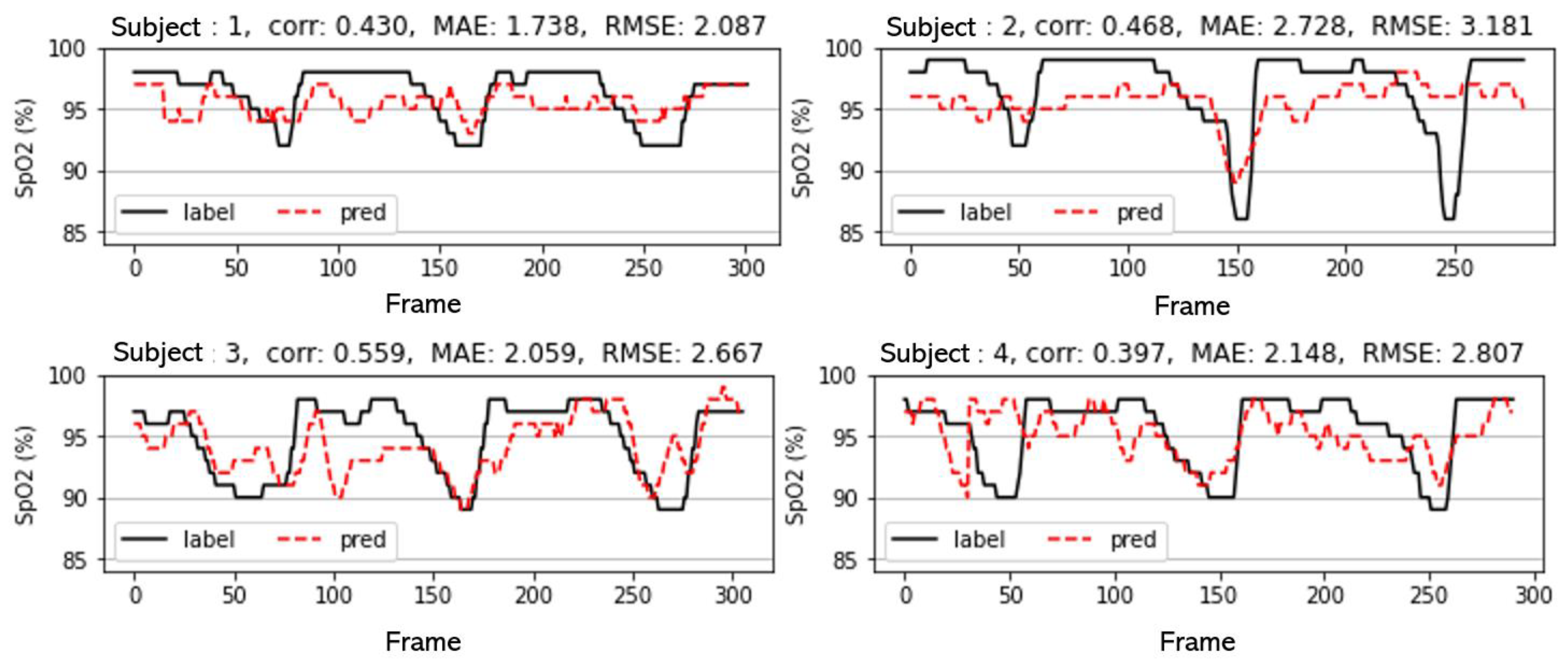
Figure 7.
Predicted oxygen saturation and actual oxygen saturation of a model trained using 10 s of signals as the input data (integrated model). For each subject, three indices were measured: corr, MAE, and RMSE: “corr” stands for the Pearson correlation coefficient, MAE stands for the “mean absolute error”, and RMSE stands for the “root mean square error”.
Figure 8.
Predicted oxygen saturation and actual oxygen saturation of a model trained using 20 s of signals as the input data (integrated model).
Figure 8.
Predicted oxygen saturation and actual oxygen saturation of a model trained using 20 s of signals as the input data (integrated model).
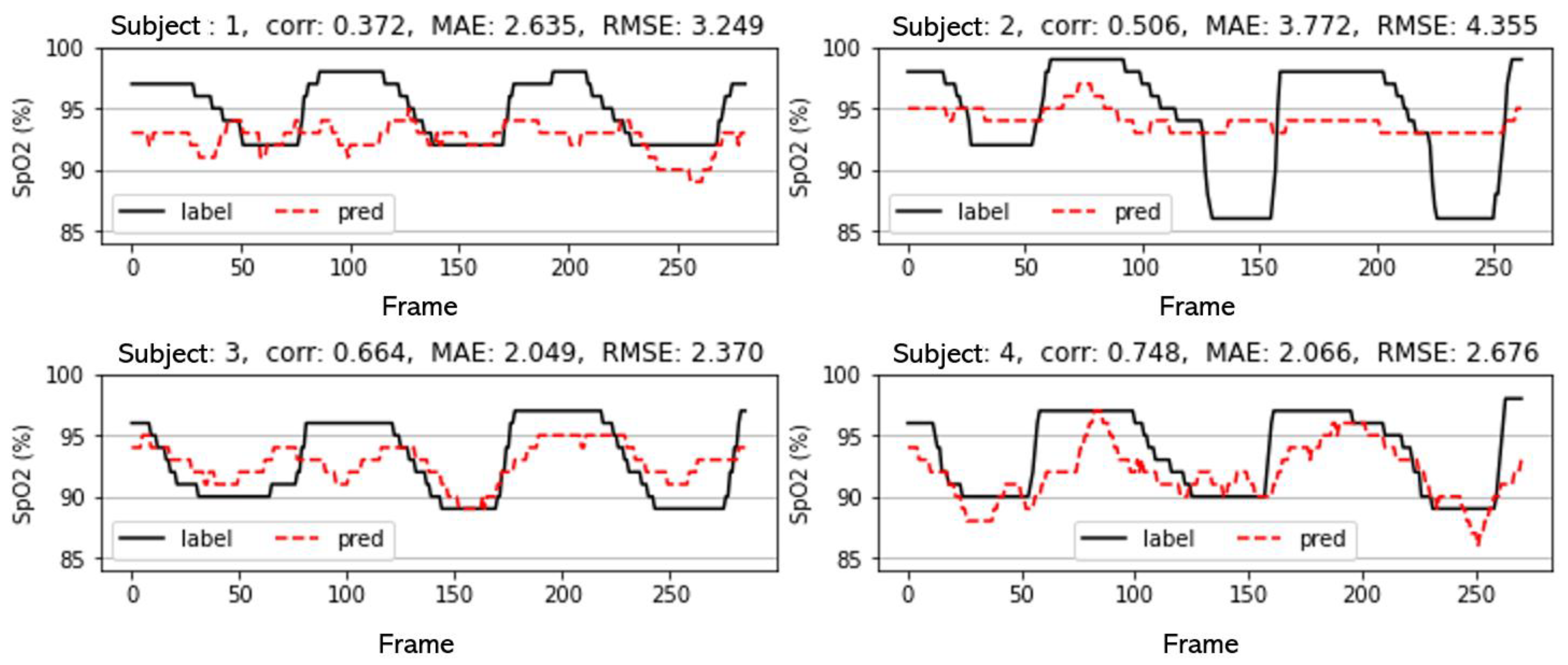
Figure 9.
Predicted oxygen saturation and actual oxygen saturation of a model trained using 30 s of signals as the input data (integrated model).
Figure 9.
Predicted oxygen saturation and actual oxygen saturation of a model trained using 30 s of signals as the input data (integrated model).
Figure 10.
Predicted oxygen saturation and actual oxygen saturation of a model trained using 10 s of signals as the input data (personalized model).
Figure 10.
Predicted oxygen saturation and actual oxygen saturation of a model trained using 10 s of signals as the input data (personalized model).
Figure 11.
Predicted oxygen saturation and actual oxygen saturation of a model trained using 20 s of signals as the input data (personalized model).
Figure 11.
Predicted oxygen saturation and actual oxygen saturation of a model trained using 20 s of signals as the input data (personalized model).
Figure 12.
Predicted oxygen saturation and actual oxygen saturation of a model trained using 30 s of signals as the input data (personalized model).
Figure 12.
Predicted oxygen saturation and actual oxygen saturation of a model trained using 30 s of signals as the input data (personalized model).
Figure 13.
SHAP values of the personalized model used in
Figure 10. The
x-axis represents the features and the
y-axis shows the contribution according to the features. Among them, the orange bar is the feature with the greatest contribution.
Figure 13.
SHAP values of the personalized model used in
Figure 10. The
x-axis represents the features and the
y-axis shows the contribution according to the features. Among them, the orange bar is the feature with the greatest contribution.
Figure 14.
SHAP values of the personalized model used in
Figure 11.
Figure 14.
SHAP values of the personalized model used in
Figure 11.
Figure 15.
SHAP values of the personalized model used in
Figure 12.
Figure 15.
SHAP values of the personalized model used in
Figure 12.
Figure 16.
SHAP values for the training and testing data of a model trained with 10 s of signals as the input data.
Figure 16.
SHAP values for the training and testing data of a model trained with 10 s of signals as the input data.
Figure 17.
SHAP values for the training and testing data of a model trained with 20 s of signals as the input data.
Figure 17.
SHAP values for the training and testing data of a model trained with 20 s of signals as the input data.
Figure 18.
SHAP values for the training and testing data of a model trained with 30 s of signals as the input data.
Figure 18.
SHAP values for the training and testing data of a model trained with 30 s of signals as the input data.
Table 1.
Summary of the related works.
Table 1.
Summary of the related works.
| Method | Author | Result |
|---|
| Metric | Value |
|---|
Use two
waves | Face ROI | Calculate the RoR and measure the oxygen saturation by estimating the AC and DC components for red and blue wavelengths | Tarassenko et al. [12] | Corrcoef | −0.8 |
| Calculate the RoR and measure the oxygen saturation by estimating the AC and DC components for red and blue wavelengths | Rahman et al. [13] | Corrcoef | 0.95 |
| Hand ROI | Calculate the RoR and measure the oxygen saturation by estimating the AC and DC components for red and blue wavelengths | Sun et al. [14] | | 0.87 |
| Use three waves | Face ROI | Calculate the AC and DC components and measure the oxygen saturation using all red, green, and blue wavelengths | Wei et al. [15] | Corrcoef | 0.68 |
| Hand ROI | Calculate the AC and DC components and measure the oxygen saturation using all red, green, and blue wavelengths | Tian et al. [16] | MAE | 1.26 |
| CNN | Face ROI | The space-time map is input to the CNN model using the AC and DC components calculated using the data of the red, green, and blue wavelengths. | Akamatsu et al. [17] | Corrcoef | 0.496 |
Table 2.
Demographic characteristics and the average values of the Cg and Cb color channels for the participants.
Table 2.
Demographic characteristics and the average values of the Cg and Cb color channels for the participants.
| ID | Gender | Age | Nationality | Cb Channel
Average | Cr Channel
Average |
|---|
| 1 | Male | 25 | Korean | 116.0 | 145.6 |
| 2 | Female | 25 | Korean | 115.0 | 143.5 |
| 3 | Male | 27 | Korean | 118.0 | 143.3 |
| 4 | Male | 27 | Korean | 117.4 | 142.8 |
| 5 | Female | 26 | Korean | 116.9 | 142.7 |
| 6 | Female | 30 | Korean | 117.3 | 142.8 |
| 7 | Male | 28 | Korean | 117.5 | 143.1 |
| 8 | Female | 24 | Korean | 117.6 | 144.0 |
| 9 | Female | 24 | Korean | 117.6 | 143.6 |
| 10 | Female | 25 | Korean | 120.1 | 140.6 |
| 11 | Male | 26 | Korean | 118.0 | 142.5 |
| 12 | Male | 28 | Korean | 114.9 | 143.9 |
| 13 | Male | 27 | Korean | 115.0 | 144.4 |
| 14 | Male | 32 | Korean | 114.0 | 146.3 |
Table 3.
Statistical results of a model trained using 10 s of signals as the input data (integrated model). For each subject, three indices were measured: the correlation coefficient, MAE, and RMSE: “correlation coefficient” stands for the Pearson correlation coefficient, MAE stands for the “mean absolute error”, and RMSE stands for the “root mean square error”.
| Subject | Correlation
Coefficient | MAE | RMSE |
|---|
| 1 | 0.430 | 1.738 | 2.087 |
| 2 | 0.468 | 2.728 | 3.181 |
| 3 | 0.559 | 2.059 | 2.667 |
| 4 | 0.397 | 2.148 | 2.807 |
| 5 | 0.502 | 3.208 | 3.649 |
| 6 | 0.417 | 3.482 | 3.782 |
| 7 | 0.500 | 3.987 | 4.763 |
| 8 | 0.569 | 2.812 | 3.201 |
| 9 | 0.337 | 3.358 | 3.979 |
| 10 | 0.476 | 3.021 | 3.623 |
| 11 | 0.294 | 1.550 | 2.035 |
| 12 | 0.200 | 1.358 | 1.691 |
| 13 | 0.357 | 2.375 | 2.980 |
| 14 | 0.294 | 2.463 | 3.060 |
| Mean | 0.414 | 2.592 | 3.108 |
Table 4.
Statistical results of a model trained using 20 s of signals as the input data (integrated model).
Table 4.
Statistical results of a model trained using 20 s of signals as the input data (integrated model).
| Subject | Correlation
Coefficient | MAE | RMSE |
|---|
| 1 | 0.586 | 0.825 | 6.338 |
| 2 | 0.512 | 3.062 | 3.816 |
| 3 | 0.696 | 1.760 | 2.373 |
| 4 | 0.672 | 5.840 | 6.343 |
| 5 | 0.496 | 2.461 | 2.978 |
| 6 | 0.582 | 6.102 | 6.692 |
| 7 | 0.512 | 3.320 | 3.678 |
| 8 | 0.377 | 3.746 | 4.259 |
| 9 | 0.241 | 5.033 | 5.852 |
| 10 | 0.468 | 7.690 | 8.289 |
| 11 | 0.594 | 4.260 | 4.737 |
| 12 | 0.378 | 2.413 | 2.903 |
| 13 | 0.056 | 3.762 | 4.459 |
| 14 | 0.448 | 3.888 | 4.437 |
| Mean | 0.473 | 3.869 | 4.797 |
Table 5.
Statistical results of a model trained using 30 s of signals as the input data (integrated model).
Table 5.
Statistical results of a model trained using 30 s of signals as the input data (integrated model).
| Subject | Correlation
Coefficient | MAE | RMSE |
|---|
| 1 | 0.372 | 2.635 | 3.249 |
| 2 | 0.506 | 3.772 | 4.355 |
| 3 | 0.664 | 2.049 | 2.370 |
| 4 | 0.748 | 2.066 | 2.676 |
| 5 | 0.529 | 1.855 | 2.264 |
| 6 | 0.584 | 3.628 | 4.050 |
| 7 | 0.492 | 2.993 | 3.360 |
| 8 | 0.475 | 3.190 | 3.788 |
| 9 | 0.395 | 5.662 | 6.489 |
| 10 | 0.401 | 5.686 | 6.168 |
| 11 | 0.570 | 1.720 | 2.390 |
| 12 | 0.199 | 1.785 | 2.079 |
| 13 | 0.238 | 2.714 | 3.438 |
| 14 | 0.481 | 2.598 | 2.981 |
| Mean | 0.475 | 3.025 | 3.547 |
Table 6.
Statistical results of a model trained using 10 s of signals as the input data (personalized model).
Table 6.
Statistical results of a model trained using 10 s of signals as the input data (personalized model).
| Subject | Correlation
Coefficient | MAE | RMSE | ICC | 95% Confidence Interval |
|---|
| 1 | 0.498 | 1.487 | 1.874 | 0.592 | 0.487~0.675 |
| 2 | 0.513 | 1.774 | 3.186 | 0.562 | 0.369~0.686 |
| 3 | 0.693 | 2.212 | 2.684 | 0.763 | 0.524~0.862 |
| 4 | 0.759 | 3.990 | 4.510 | 0.601 | −0.213~0.852 |
| 5 | 0.451 | 1.343 | 1.922 | 0.615 | 0.517~0.693 |
| 6 | 0.653 | 1.741 | 1.973 | 0.434 | −0.196~0.751 |
| 7 | 0.509 | 2.378 | 2.828 | 0.375 | −0.184~0.662 |
| 8 | 0.620 | 1.718 | 2.279 | 0.677 | 0.597~0.742 |
| 9 | 0.411 | 0.872 | 1.374 | 0.297 | 0.005~0.494 |
| 10 | 0.576 | 0.357 | 0.694 | 0.714 | 0.639~0.773 |
| 11 | 0.713 | 1.082 | 1.444 | 0.770 | 0.710~0.817 |
| 12 | 0.403 | 2.735 | 3.238 | 0.353 | 0.004~0.564 |
| 13 | 0.496 | 1.267 | 1.709 | 0.538 | 0.418~0.632 |
| 14 | 0.684 | 1.618 | 2.255 | 0.743 | 0.631~0.815 |
| Mean | 0.570 | 1.755 | 2.284 | 0.574 | - |
Table 7.
Statistical results of a model trained using 20 s of signals as the input data (personalized model).
Table 7.
Statistical results of a model trained using 20 s of signals as the input data (personalized model).
| Subject | Correlation
Coefficient | MAE | RMSE | ICC | 95% Confidence Interval |
|---|
| 1 | 0.579 | 1.558 | 1.922 | 0.664 | 0.577~0.733 |
| 2 | 0.669 | 2.125 | 3.199 | 0.750 | 0.682~0.803 |
| 3 | 0.516 | 2.980 | 3.638 | 0.636 | 0.467~0.742 |
| 4 | 0.817 | 3.014 | 3.465 | 0.725 | −0.189~0.907 |
| 5 | 0.512 | 1.935 | 2.555 | 0.586 | 0.293~0.737 |
| 6 | 0.767 | 1.044 | 1.257 | 0.678 | −0.195~0.882 |
| 7 | 0.572 | 1.490 | 2.040 | 0.620 | 0.519~0.700 |
| 8 | 0.688 | 2.214 | 2.934 | 0.603 | 0.389~0.729 |
| 9 | 0.269 | 1.165 | 1.570 | 0.369 | 0.174~0.513 |
| 10 | 0.723 | 0.630 | 0.858 | 0.816 | 0.756~0.859 |
| 11 | 0.756 | 1.157 | 1.586 | 0.827 | 0.713~0.887 |
| 12 | 0.577 | 1.224 | 1.560 | 0.687 | 0.567~0.768 |
| 13 | 0.671 | 1.308 | 1.706 | 0.787 | 0.709~0.841 |
| 14 | 0.698 | 2.241 | 2.772 | 0.783 | 0.612~0.865 |
| Mean | 0.630 | 1.720 | 2.219 | 0.681 | - |
Table 8.
Statistical results of a model trained using 30 s of signals as the input data (personalized model).
Table 8.
Statistical results of a model trained using 30 s of signals as the input data (personalized model).
| Subject | Correlation
Coefficient | MAE | RMSE | ICC | 95% Confidence Interval |
|---|
| 1 | 0.727 | 1.812 | 2.313 | 0.613 | 0.112~0.797 |
| 2 | 0.231 | 4.715 | 6.120 | 0.363 | 0.191~0.498 |
| 3 | 0.626 | 2.853 | 3.200 | 0.590 | 0.085~0.783 |
| 4 | 0.845 | 2.343 | 2.939 | 0.854 | 0.697~0.917 |
| 5 | 0.821 | 2.837 | 3.336 | 0.706 | 0.376~0.836 |
| 6 | 0.440 | 1.775 | 2.210 | 0.428 | 0.105~0.617 |
| 7 | 0.562 | 1.074 | 1.445 | 0.686 | 0.589~0.758 |
| 8 | 0.700 | 2.412 | 3.105 | 0.614 | 0.423~0.731 |
| 9 | 0.759 | 0.857 | 1.152 | 0.840 | 0.785~0.879 |
| 10 | 0.636 | 2.376 | 2.638 | 0.385 | −0.196~0.707 |
| 11 | 0.688 | 1.428 | 1.766 | 0.775 | 0.681~0.837 |
| 12 | 0.797 | 0.676 | 0.855 | 0.850 | 0.790~0.891 |
| 13 | 0.618 | 3.025 | 3.392 | 0.505 | −0.215~0.782 |
| 14 | 0.828 | 1.804 | 2.092 | 0.831 | 0.785~0.867 |
| Mean | 0.663 | 2.142 | 2.612 | 0.646 | - |
Table 9.
Summary of the oxygen saturation prediction results according to the input data lengths.
Table 9.
Summary of the oxygen saturation prediction results according to the input data lengths.
| | Correlation Coefficient | MAE | RMSE |
|---|
| Integrated Model | 10 s | 0.414 | 2.592 | 3.108 |
| 20 s | 0.473 | 3.869 | 4.797 |
| 30 s | 0.475 | 3.025 | 3.547 |
| Personalized Model | 10 s | 0.570 | 1.755 | 2.284 |
| 20 s | 0.630 | 1.720 | 2.219 |
| 30 s | 0.663 | 2.142 | 2.612 |
| Previous Research [15] | 0.680 | - | 1.819 |
| Previous Research [17] | 0.496 | 1.18 | 1.4 |
| Disclaimer/Publisher’s Note: The statements, opinions and data contained in all publications are solely those of the individual author(s) and contributor(s) and not of MDPI and/or the editor(s). MDPI and/or the editor(s) disclaim responsibility for any injury to people or property resulting from any ideas, methods, instructions or products referred to in the content. |
© 2024 by the authors. Licensee MDPI, Basel, Switzerland. This article is an open access article distributed under the terms and conditions of the Creative Commons Attribution (CC BY) license (https://creativecommons.org/licenses/by/4.0/).


