Transportation Simulation Modeling and Location-Based Services Data Completion Based on a Data and Model Dual-Driven Approach

Abstract

The evolving economic and technological landscape has brought about significant changes in travel behaviors and traffic patterns. These changes have led to the emergence of complex, multi-modal travel demands that interact with transportation networks, posing new challenges in transportation analysis and control. The primary objective of this study is to address these challenges by improving transportation modeling and data completeness using advanced modeling tools and transportation big data. We propose a dual-driven simulation model that integrates transportation simulation and big data. The approach begins by utilizing initial Location-Based Services (LBS) data to establish a mesoscopic multi-modal simulation model, which is then calibrated. This calibrated model is then employed to complete the missing trajectories of the LBS data. The innovative aspect of this dual-driven simulation model lies in its novel approach to constructing transportation models and completing LBS data, thereby enhancing both the simulation accuracy and the results of missing path completion. We conduct tests using the urban area of Hangzhou as an example, and the results show that the Normalized Root Mean Square Error (NRMSE) between the average link speeds in the simulation model and in real world observation is reduced to 24.1%. In the LBS data completion process, our proposed method achieves a travel mode identification accuracy of 95.3% for private car travel. Compared to the two baseline methods, the average accuracy of completed trajectories increases by 6.31% and 2.46%, respectively.

1. Introduction

With the development of the economy and technology, the scenarios of people traveling and traffic flow have been changing over time. The complex multi-modal travel demand and corresponding interactions with multi-modal transportation networks bring new challenges to system-wide transportation analysis, deduction, and control. Both advanced system modeling tools and transportation big data are required to fulfill the aforementioned tasks. All along, transportation simulation has a rich accumulation in the literature [1,2,3,4], and transportation data-driven studies have been attracting attention recently. Therefore, the fusion of transportation simulation and transportation big data, i.e., model and data dual-driven simulation, will make a difference.

Transportation simulation is an essential approach to understanding and predicting traffic dynamics of city-wide transportation networks. It can capture the complex interactions between different elements in transportation systems, evaluate and compare the influences of different planning schemes, and assist the design of operations management strategies to seek the optimal solution to transportation problems [5,6,7]. Over the years, there has been a significant shift in the transportation modeling paradigm. The traditional Four-Stage Models have evolved into more advanced Activity-Based Models. Concurrently, modeling approaches have shifted from static to dynamic models [8], expanding from a macroscopic perspective to a microscopic level. Additionally, there has been a transition from discrete-event models to agent-based models [7,9]. These transformations have led to more complex data required for transportation simulations. Consequently, the acquisition and processing of such complex data have become a major bottleneck for system modeling. Recently, the emergence of data-driven simulation has offered a promising solution, which leverages massive amounts of data generated using transportation systems to develop models that are more accurate and efficient [10]. By relying on data-driven simulations, researchers can capture the complexity of transportation systems while minimizing the need for extensive manual data collection and processing.

The field of transportation planning has evolved significantly with the advent of big data. Initially, transportation planning research primarily relied on traditional travel survey data for information gathering [11], constrained by limitations such as insufficient sample sizes and poor data real-time performance. With the advancements in information technology, numerous sources of real-time data have become available for modeling purposes, such as traffic flow data from checkpoints [12], mobile signaling data [13], and public transit card swiping data [14]. Moreover, the rise of Location-Based Services (LBS) data has introduced new possibilities and advantages. LBS data provide detailed information on individuals’ spatial and temporal behaviors, allowing for a more granular understanding of travel demand patterns. It gains insights into origin–destination (OD) flows, route choices, and mode selection, among other valuable information. Recently, a growing number of studies have used LBS data from telecom carriers, smartphone-based apps, and Bluetooth devices for transportation applications [15,16]. However, due to insufficient data coverage, data-network mismatching and privacy issues, the usage of LBS data in transportation studies is still in its infancy, necessitating further dedicated research. Such issues need to be addressed to ensure data robustness and reliability. To tackle these challenges, mitigating potential data gaps and ensuring data integrity is imperative. Currently, the completion of LBS data primarily relies on statistical learning and machine learning, with no existing method for data completion through transportation simulation. This gap in the research represents a significant opportunity for exploration and innovation.

This paper proposes a model and data dual-driven transportation modeling approach based on simulation model development and LBS data-driven analysis. Using the mesoscopic simulation software MATSim (v.13.0) as a case study, the proposed approach is evaluated through the utilization of LBS data provided using AMap (https://ditu.amap.com/, accessed on 12 October 2022), a leading digital map and navigation service provider in China. First, the original LBS data with partly missing information (trajectories and mode choices in some trips) are used to extract the initial travel demand and link/route traffic information, and the information is utilized to build and calibrate a mesoscopic multi-modal transportation simulation model, which reflects the actual traffic conditions. Second, the calibrated simulation model is adopted to complete the missing information in the original LBS, which achieves simulation-based data completion and the recalibration of the initial multi-modal travel demand.

The main contributions of this paper are threefold: (a) Solving the problem of data dependence and data completion for transportation simulation development simultaneously; (b) the dual-driven simulation model (DDSM) provides a new paradigm for the construction of subsequent transportation simulation models and the completion of LBS data; (c) the completion process of DDSM has a higher accuracy for recognizing travel modes, and the completion of missing travel paths is more authentic and reliable than other methods. We tested our proposed DDSM in the urban area of Hangzhou, and the results demonstrated that our algorithm outperforms other completion algorithms in LBS data complement.

The remainder of this paper is organized as follows. Section 2 reviews the transportation simulation modeling methods and LBS data completion methods. Section 3 describes the research methodology for traffic simulation modeling and calibration, as well as LBS data completion, based on a dual-drive approach incorporating both data and models. In Section 4, we analyze the results of multi-modal simulation modeling and calibration, as well as simulation-based data completion. We show the model calibration and data completion performance compared to other completion algorithms. Concluding remarks and future work are presented in Section 5.

2. Literature Review

2.1. Data-Driven Transportation Simulation

Transportation simulation has been a long-standing tool for system analysis, which uses computer digital models/methods to reflect complex traffic phenomena. According to the resolution level of the system, transportation simulation models can be classified into three types: macroscopic, mesoscopic, and microscopic simulation. The comparison of them is summarized in

Table 1. Comparison of macro-, meso-, and micro-simulation models.

Simulation Model	Common Software	Granularity	Object Description	Ease of Data Fusion
Macroscopic simulation	TransCAD [17,18], VISUM [19]	lower	traffic flow	lower
Mesoscopic simulation	MATSim [20], DTALite [21], DynusT [22,23]	medium	specific vehicles	medium
Microscopic simulation	VISSIM [24], SUMO [25]	higher	each vehicle	higher

.

Macroscopic models consider traffic flow as a continuous stream and plan the regional or overall city traffic layout. These models primarily focus on general traffic flow trends and macroscopic characteristics, e.g., traffic volume, velocity, and density. The study utilized TransCAD to estimate evacuation and sheltering demands [17]. The study used VISUM to implement urban public transport allocation [26]. Macroscopic simulation requires a few network data (e.g., basic road topology, fundamental road segment attributes, road segment capacity, and free-flow speed.), and uses survey data as the input for OD demand. The study incorporated road network information (nodes, zones, and links within Dublin city) from VISUM and the Irish National Transport Model into its macroscopic simulation. Travel demand data encompassed OD matrix data in the form of both cars and heavy goods vehicles [27].

Based on the macroscopic traffic network, mesoscopic models position individual vehicles within the macroscopic flow to estimate traffic conditions. It emphasizes traffic flow and vehicle interactions over a broader area, and reveals metrics such as traffic volume distribution, vehicle travel times, and delays. The study employed DynusT to evaluate the system performance of different link toll schemes on real highways [22]. DTAlite [28] and MATSim [20] are widely used in multi-modal systems for their flexibility and ease of customization offered using open-source software. Compared to macroscopic simulation models, mesoscopic simulation requires higher data resolution, such as detailed road topology and lane configuration in road network data. The study utilized road network and demand data provided by the government officially. The researchers highlighted the potential use of more detailed preference data for developing and calibrating more sophisticated travel demand models under evacuation scenarios.

Microscopic models focus on the interaction between each vehicle/traveler. The study rigorously evaluated various signal phase settings using the developed system interfaced with CORSIM microsimulation [29]. The study estimated the vehicle states based on connected vehicle data and simulated a real intersection in VISSIM for testing [30]. Transmodeler was applied to match vehicles operating characteristics for the purpose of emissions reduction and safety [31,32]. Microscopic simulation has the most rigorous demand for network data, requiring complete road geometries and traffic signal timing data. It also requires detailed time-dependent traffic demand data, such as route choice, trip chaining, and vehicle attribute data.

Recently, research focus has gradually shifted from single simulation to hybrid simulation, i.e., macro- and micro-integrated transportation modeling and simulation [33], and meso- and micro-integrated simulation [34]. Additionally, with the rapid development of intelligent transportation systems (ITS), the volume of traffic data has surged significantly, driving transportation simulation towards a more data-driven direction with better data utilization, making the application of data in traffic simulation more extensive and profound. Regarding road networks, OpenStreetMap (https://www.openstreetmap.org/, accessed on 12 October 2022) (OSM) is a frequently used road network data source. As for travel demand, fast-growing communication networks and positioning systems have promoted the emergence of LBS data. Data development improves the accuracy and diversity of transportation simulation. This, in turn, enables exploring a more comprehensive range of application scenarios and possibilities, providing enhanced support and guidance for transportation planning and management.

Table 2. Data-driven transportation simulation.

Researchers	Simulation Demand Data	Simulation Network Data	Main Work
Griggs et al. [10]	Real and virtual vehicle	Network of the local University’s campus	Present a simulation platform to examine real-world driver responses to feedback control.
Zhang et al. [16]	GPS (LBS)	Network of Shanghai	Highlight the potential of MATSim in simulating large-scale dynamic transport scenarios.
Horl and Balac [35]	Census data set	Network of Paris and its surroundings	Introduce the process for generating a synthetic travel demand based on open data/software.
Gurrame et al. [15]	Phone GPS (LBS)	Network of the entire North America	Illustrate the value of data-driven simulations in estimating and predicting travel demand.
Patel et al. [36]	Virtual vehicle	Two roads (34 km and 8 km) in the city	Upgrade the SiMTraM model to better suit Indian traffic scenarios.
Onelcin et al. [37]	Survey data	Network of the town with a petrochemical enterprise	Conduct evacuation time estimates and obtain reliable evacuation simulation results.

presents a summary of some previous simulation models’ data sources and simulation scales. Conventionally, traditional transportation simulation modeling mainly relies on non-LBS data (data not based on Location-Based Services), which has several disadvantages: First, its limited resolution undermines the precision required for accurate simulations. Second, the inability to update in real-time hinders the timely reflection of changing traffic conditions. Third, the spatial resolution is limited, and it is difficult to delicately depict the traffic network. Additionally, spatial resolution constraints hinder the detailed depiction of the traffic network. Finally, the difficulty in capturing individual behaviors and external factors closely related to traffic metrics results in discrepancies between simulation outcomes and real-world scenarios. For accuracy, researchers are exploring the adoption of LBS data sources such as data from telecom carriers, smartphone-based apps, and Bluetooth devices. A few studies have fully used geospatially accurate Global Positioning System (GPS) data for the simulation [15,16]. However, they only retain the start and end point information of GPS data, and discard the key waypoint data extracted from GPS data during the research process. Both methods fail to fully utilize the precise information provided using LBS (such as the individual’s actual route choices), which not only affects the accuracy of the simulation, but also increases the complexity and difficulty of subsequent model calibration.

2.2. LBS Data Completion

In practice, the availability and efficiency of LBS data are hindered by issues such as detector malfunctions, adverse weather conditions, and communication system failures. The partial absence of movement trajectory is a common occurrence. Specifically, within a specific time period, intermediate details in the travel (positional information and timestamp data) are missing, and only the OD information is retained. This situation seriously disrupts data continuity, making it impossible to accurately reconstruct the traveler’s path choice and travel mode. Hence, it becomes necessary to employ specific technical methods to supplement the incomplete data, a process known as LBS data completion.

Based on the idea of the shortest path method, the study proposed a macro–micro-integrated framework, combining particle filter (PF) and path flow estimation (PFE) to reconstruct the running path of vehicles. Their experiments with the VISSIM simulation model showed outstanding performance over a single PFE model [38]. The study proposed a trajectory-matching algorithm for emission-exceeding vehicles based on network topology and weights. Researchers select a group of adjacent matching trajectory candidate road segments using topological and spatial constraints. A composite weight, considering factors such as distance, direction, and relative position relationships, is then calculated for each candidate segment as its new evaluation criterion. Finally, the Dijkstra algorithm is employed to obtain the optimal matching path sequence based on these weights [39]. A researcher used the topological optimization based on the speed constraint (SC + TO) method combined with the technique for order preference by similarity to the ideal solution method (TOPSIS) to complete the extraction and reconstruction of vehicle travel paths [40]. The study constructed the feasible solution set of travel paths based on the K-th shortest paths algorithms (KSP). By establishing indicators such as path distance, travel time consistency, the number of signalized intersections, the degree of path preference, number of turns, and other decision indicators, the gray relational algorithm (GRA) determines the optimal completion path with a comprehensive accuracy of 92% [41]. Based on the idea of semi-supervised learning, the study constructed a path selection model based on sparse data by estimating the parameters of the maximum likelihood function. The experimental results showed that the method effectively improved the accuracy of the path selection model [42].

In the era of transportation big data, traditional methods (e.g., shortest path method and topology optimization method based on speed limit) are not satisfactory for LBS travel path completion. Machine learning algorithms can explore the complex relationships behind data, but due to their black-box nature, subsequent analysis often lacks sufficient theoretical and model support, limiting the ability to understand and optimize model behavior. The emergence of multi-modal transportation (including bike-sharing and ride-sharing) has posed challenges in finding the most efficient path, as traditional methods only consider one travel mode. Completing a travel path using LBS involves various factors, e.g., traffic conditions, weather, road closures, and construction. Traditional methods that rely solely on speed limits or road topology are insufficient to address these complex scenarios effectively. Therefore, it is of great significance to establish a new modeling approach to improving imputation accuracy for missing travel paths in large-scale LBS data.

2.3. Summary

To this end, the development of simulations emphasizes the use of multi-modal options and trip chains. Traditional non-LBS data modeling has significant limitations due to the difficulties and high costs in obtaining multi-modal intermodal survey data. As a result, modeling with LBS for simulation purposes has become a trend in urban transportation systems. Simultaneously, LBS data quality issues need to be addressed via methods that offer better interpretability, accuracy, and reflection of real-world situations. In conclusion, the dual-driven simulation modeling (DDSM) approach can effectively address both issues.

3. Materials and Methods

3.1. Flowchart of the Dual-Driven Simulation Model

The flowchart of the proposed DDSM is presented in Figure 1. The initial data needed for the model are the demand and supply of the transportation network. The transportation demand data consist of trip chains from LBS data, and the actual traffic flow is obtained via extracting the travel chain information. The supply data of the transportation network includes the road network topology and public transportation hubs, which together constitute the facility foundation for transportation operations. Given the initial data, the development of DDSM includes three major steps: model initialization, model calibration, and LBS missing path completion. Model initialization is a preparatory process that begins with selecting the study area, followed by filtering and processing the aforementioned raw data according to the spatial-temporal coverage, ultimately completing model construction. Model calibration is the process of enhancing the credibility and predictive capability of simulation models using LBS data. The calibration goal is to align the outputs of simulation models as closely as possible with observed data, primarily through supply calibration (identifying and calibrating the incorrect values of road speed limits and capacities) and demand adjustment (selecting key road segments for demand adjustment based on the error between actual and simulated traffic conditions, and subsequently scaling the OD demand of passing these road segments) to minimize the discrepancies between simulated and observed traffic attributes. This process helps to improve the fitting degree of the model to the actual traffic conditions. A completion operation is performed to address the missing path issue in the LBS data. Specifically, the calibrated model is used to generate optional driving paths for LBS trips with missing paths. The reliability of each path is then evaluated based on relevant indicators such as travel time, and the best path is selected for completion. After completion, the differences between simulated and actual traffic attributes are reassessed. If the path completion deteriorates the calibration results (with the new error exceeding a preset threshold), the calibration process is revisited, and demand adjustment is performed again. Finally, a performance check is conducted on the completed data to analyze the accuracy and effectiveness of the completion results.

3.2. Data Acquisition

The proposed DDSM requires supply and demand data, which refer to road network, public transit, and LBS demand data.

Road network data is a collection of information about roads, typically used in the applications such as geographic information system, transportation planning, traffic simulation, and navigation systems, and can be obtained through open data platforms like Google Maps API and OSM. To acquire precise road network data, this study drew upon comprehensive data resources from AMap and OpenStreetMap. The information in road network data can be categorized into road segment information and key road node/intersection information. Attributes of road segment information include link name (or link ID), length, width, speed limit, level, type, and number of lanes. Key road node/intersection information includes intersection ID, intersection coordinates (latitude and longitude), as well as the latitude (lat) and longitude (lon) of key nodes for road alignment between intersections. Aside from the foundational road network data mentioned above, a multi-modal road network also requires public transportation information, including bus and subway operational information. The pertinent details pertaining to public transportation routes and schedules were gathered from AMap, along with the official online platforms of local public transportation operators. These data primarily encompass public transit schedules (departure times and estimated arrival times), route planning, station waiting times, the coordinates of stations (latitude and longitude), and public transit vehicle information.

In addition to multi-modal road network data, LBS data are needed for modeling OD and mode-level travel demand in the network. LBS data collection typically begins with users using devices or applications equipped with location-aware capabilities (e.g., social media, navigation apps, and weather apps), which acquire the geographical coordinates of the device/user along with timestamp information. The LBS data obtained in this paper were derived from the navigation data of AMap in Hangzhou City, Zhejiang Province. The data recorded the navigation trajectory information generated by users when using AMap from 23 to 29 May 2022. Taking into account the protection of user privacy, the data anonymized identifiable information such as user IDs, while preserving the user’s spatial-temporal trajectory points, travel modes, and the travel duration of the entire trip. The more densely detailed LBS data that record the traveler’s frequent travel trajectory points make it possible to infer the traveler’s travel path (e.g., information about the sequence of road segments entered and entry times). However, the accrual path information of some trajectories is missing. It is challenging to infer due to the large number of alternative routes connecting the OD pair. The data with missing trajectories are the target for LBS data path completion.

3.3. Model Initialization

We select MATSim, an open-access mesoscopic simulation package, as the simulation platform for developing DDSM. As a dynamic and agent-based transportation simulation, MATSim allows for large-scale simulations (with millions of agents) and supports multi-modal scenarios (including private cars and public transportation). With versatile analysis and simulation outputs, MATSim is suitable for extending algorithms for model calibration and LBS path completion.

3.3.1. Study Area Selection

To develop DDSM via MATSim, we need to filter and process initial demand and supply data. Since coverage areas of road network raw data and LBS that demand raw data are inconsistent, we first select a study area and perform temporal and spatial filtering of the raw data according to the area scope. We selected a study area in Hangzhou, China, the host city of the 19th Asian Games in 2023. The research area covers an approximate area of 46.5 square kilometers above the Rainbow Expressway in Binjiang District of Hangzhou, including the river crossing road at the edge of the region. According to local government statistical yearbooks, the resident population within this area was about 338,000 people in the year 2021.

3.3.2. Data Processing

MATSim requires an initial travel demand plan, which includes detailed fixed-place activities (e.g., home, work, shopping), their locations, start times, and durations for each agent (traveler). These plans are loaded into the travel network for route planning and travel mode assignment, while travel paths and modes can also be predefined. It allows for better integration with LBS data and supports various multi-modal travel options. We perform the following data processing steps to convert the original data to MATSim demand and supply files.

(a) Adaptation of Supply Data to Simulation Modeling.

The road network is stored in the format of XML (Extensible Markup Language), consisting of two core data sets: intersection nodes and roads, which correspond to vertices and edges in graph theory, respectively. The road network data in Section 3.2 and their corresponding relationships with the required network format of MATSim are shown in

Table 3. Correspondence between Initial Network and MATSim Network.

Initial Network	Road Segments						Key Road Nodes
Initial tag	name	length	limit	/	type	lanes	name	lat and lon
MATSim tag	ID	length	limit	capacity	type	lanes	ID	X and Y
MATSim Network	Links						Nodes

, in which roads and key road nodes are abbreviated as “links” and “nodes” in the simulation. The information in the road segment data can be directly mapped to similar attribute labels in MATSim. Since the original data lack “link capacity” information, we derive the capacity of links according to their levels and the number of lanes (see

Table 4. Functionality level of links in the transportation network.

Hierarchy	Highway Type	Lane Capacity (Vehicles/Hour)
1	Motorway	2000
2	Trunk	1500
3	Primary	1500
4	Secondary	1000
5	Tertiary	600

[43]). The link capacity ($L_{cap}$) is the multiplication between level-based lane capacity ($L_{lev-cap}$) and the number of lanes ($L_{lanes}$), shown as follows:

$$L_{cap}=L_{lev-cap}\ast L_{lanes}$$

(1)

The conversion from raw data format to the MATSim road network format is accomplished by utilizing the josm-matsim-plugin (https://github.com/matsim-org/josm-matsim-plugin, v.d70ae5a) in Python (v.3.8). Moreover, since the original road network data contain a large amount of non-road information and small roads with low traffic demand, it burdens our simulation in the route planning and LBS completion process. As a result, we conduct a filtering process to extract the road network information required for the simulation, excluding links with speed limits below 20 km/h, typically associated with residential area roads. After the screening process was completed, we once again conducted a thorough check and confirmation of the connectivity of the road network.

In terms of integrating public transportation supply, we utilize public transportation information data, including schedules, route planning, station waiting times, and stop locations. Public transportation vehicle information is obtained through configuring different vehicle types, seat capacities, and standing passenger capacities for various public transportation routes. By consolidating and summarizing the public transportation data along with the basic road network data, we ultimately generate a multi-modal simulation road network. The final road network encompassed both highway and railway transportation. As shown in Figure 2, the multi-modal simulation road network included 999 nodes, 1990 links (white lines), 30 public transportation routes (lines with dark blue shading), and 5 subway lines (red dashed lines), with blue dots representing public transportation stops. During the road network generation process, we used Java OSM (JOSM, v.18746) for network visualization and manual adjustments. Additionally, we utilized the josm-matsim-plugin in Python to convert the OSM format to the MATSim road network format.

(b) Adaptation of Demand Data to Simulation Modeling.

Based on the sparsity of the track points, anonymous LBS data records mentioned in Section 3.2 can be categorized into two types: one that meticulously records travelers’ detailed travel trajectory points, facilitating the easy inference of their actual travel information (referred to as Type A data in this paper), and the other records trajectory points with multiple possible map-matching path options between these points, thus making it challenging to infer their actual path information, as they are considered to include OD points only (referred to as Type B data). In Type B data, departure and arrival times are not specific timestamps but approximate time ranges. For the both types of LBS data, we first filter LBS travel records with the origin (O) or destination (D) falling within the study area. For transiting data, only the portion within the study area is considered. For Type A data, we need to obtain the travel path on the road network by associating its temporal and spatial sequences through a map-matching algorithm. Then, we generate agent plans for demand modeling using the LBS data mentioned above. We set the simulation time horizon from 6:30 a.m. to 9:30 a.m., with a warm-up period of 30 min (6:30–7:00). Specifically, the modeling area and time horizon include 50,533 Type A data records (car mode only) and Type B data (18,317 car mode and 16,324 public transportation mode) records. We only load private car travel in the initial modeling process. As a result, we obtained a total of 68,850 MATSim travel plans.

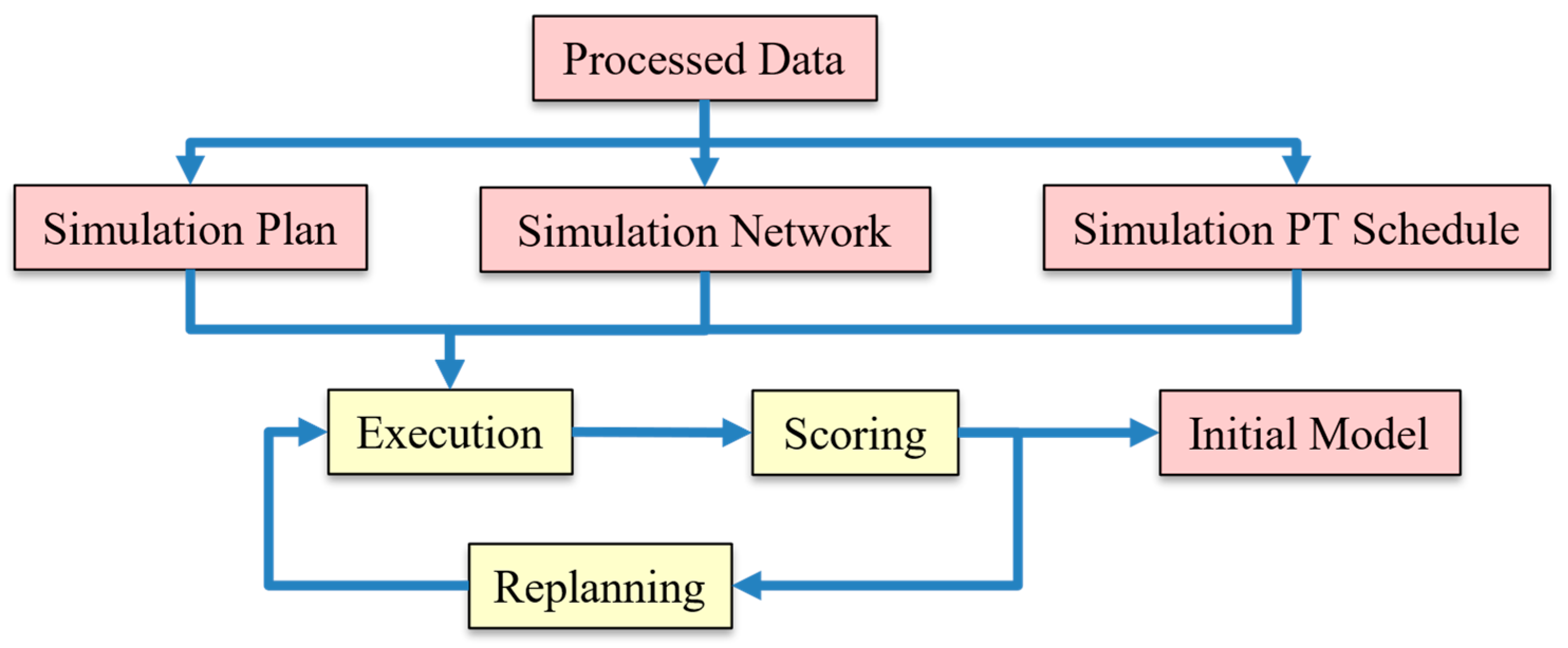
3.3.3. Model Initialization

We establish a typical model of a general day during weekdays, serving as an illustration of the methodological framework. Considering computational efficiency and application requirements, we have harmonized the time range mentioned above in Type B data (referred to as the duration of a time period) with the time range used during the calibration process, setting it to 15 min. We filter the fields such as OD coordinates, departure, and arrival times from Type A and Type B data, and organize them into the format required for MATSim plan files. In this process, the departure and arrival times for Type A data are specific timestamps recorded in the data, while for Type B data, the departure and arrival times are randomly generated within their respective time periods. Additionally, the travel path for Type A data is predefined and represented as a set of link ID sequences.

During the simulation execution, MATSim tracks the spatiotemporal movements of agents along their estimated or predefined travel routes (entry and exit timestamps for each road link) and their activity participation (start and end timestamps for each fixed location activity). This information is scored and stored in memory as events. Then, the simulated replanning process generates different potential travel scenarios, which can provide data support for the subsequent completion of LBS data. The illustration of the iterative calculation of traffic states in MATSim is shown in Figure 3.

Apart from being used in simulation model initialization, the demand data can also be extended to subsequent stages of simulation model calibration and LBS data complement validation. Specifically, information about sequentially entered road segments such as road segment IDs and entry times in Type A data provides us with travel time on each road segment. Consequently, we can calculate the actual average speed of the link as an indicator for model calibration. By intentionally creating missing path information within Type A data and forming it into a test dataset, we can assist in validating the effectiveness of the data completion methods.

3.4. Simulation Model Calibration

Model calibration is a task for any transportation simulation to estimate and reflect transportation dynamics. In the calibration process of transportation simulation models, compared to other data calibration methods, LBS data calibration poses unique challenges. Due to the limitations of LBS data coverage, not all travelers use the same app that provides LBS information, leading to incomplete capture of travel information, hindering the accurate reflection of actual traffic demand. This gap between data and real demand is difficult to narrow through adjustments to the model’s own parameters. To overcome these challenges, in addition to adjusting road attributes (such as rectifying erroneous speed limits and recalculating capacity information), we also select representative links (with trajectory data for all time periods) as the target links for simulation calibration. To capture the temporal variations in traffic conditions, a time-period-by-time-period calibration strategy is employed. By computing the average segment speed for each road segment during the current travel period, we gain a deeper understanding of the traffic conditions within that specific time period. Based on this analysis, the links exhibiting the largest errors during the current time period are identified as the key links for each calibration iteration, serving as the primary focus for adjustments to travel demand. By individually calibrating the traffic data for each time period, the model is able to more accurately reflect the temporal variations in traffic conditions, thereby enhancing its overall accuracy and reliability. Specific methods are as follows.

3.4.1. Links Selection and Evaluation Metrics for Simulation Calibration

As indicated in Section 3.3, the processed Type A data retains the actual route information of the vehicles, including the id of each link they enter and the corresponding entry time. The average speed of the vehicle on the link can be calculated as follows:

$$S_{m,i}=\frac{l_m}{U_{m,i}^{+}-U_{m,i}^{-}}$$

(2)

where $S_{m,i}$ is the average speed of vehicle $i$ on link $m$, $l_m$ is the length of link $m$, $U_{m,i}^{-}$ and $U_{m,i}^{+}$ are the moment that vehicle $i$ enters and exists link $m$ respectively.

Then, according to the 15 min time period length, the simulation time is divided into 8 periods, and the real average road speed in each period is calculated. The specific calculation method is shown as follows:

$$S_{m,t}=\frac{l_m}{{{\displaystyle \sum }}_{T_{l.i}\in t}^{N_{m,t}}\left(U_{m,i}^{+}-U_{m,i}^{-}\right)/N_{m,t}}$$

(3)

where $S_{m,t}$ is the average speed of link $m$ in time period $t$, $l_m$ is the length of link $m$, $U_{m,i}^{-}$ and $U_{m,i}^{+}$ are the moment that vehicle $i$ enters and exists link $m$ in time period $t$ respectively, and $N_{m,t}$ is the number of vehicles using this link during the time period.

Through this process, we obtain the actual average speeds of links with trajectory data passing through them during each time period. Subsequently, we select those roads that have trajectory data passing through them during all time periods as the target links for simulation calibration. Fifty target roads are chosen as the calibration objects in this study, and their distribution details are shown in Figure 4. The selection of these target roads aims to ensure that the calibration results can cover and represent the actual conditions of the entire transportation network.

Similarly, the simulation output from MATSim directly provides the entry and exit times for each vehicle on links. The simulated average link speed within can be obtained using the abovementioned methods.

In this study, Root Mean Square Error (RMSE) and Normalized Root Mean Square Error (NRMSE) are selected as evaluation metrics for simulation calibration. These metrics are primarily used to measure the magnitude of the error between the predicted average link speeds from the model and the actual observed link speeds. We count the RMSE and NRMSE between real-world and simulated speeds as follows:

$$RMS{E}_t=\frac{{{\displaystyle \sum }}_{i=1}^M{\left(S_{m,t}-S_{m,t}^{\prime }\right)}^2}{M}$$

(4)

$$NRMS{E}_t=\frac{{{\displaystyle \sum }}_{i=1}^M{\left(S_{m,t}-S_{m,t}^{\prime }\right)}^2}{{{\displaystyle \sum }}_{m=1}^M{S}_{m,t}^2}$$

(5)

where $RMS{E}_t$ and $NRMS{E}_t$ are the RMSE and NRMSE values of time period $t$ respectively, $S_{m,t}^{\prime }$ is the simulated average speed of link $m$ in time period $t$, and $M$ is the number of target links selected for calibration.

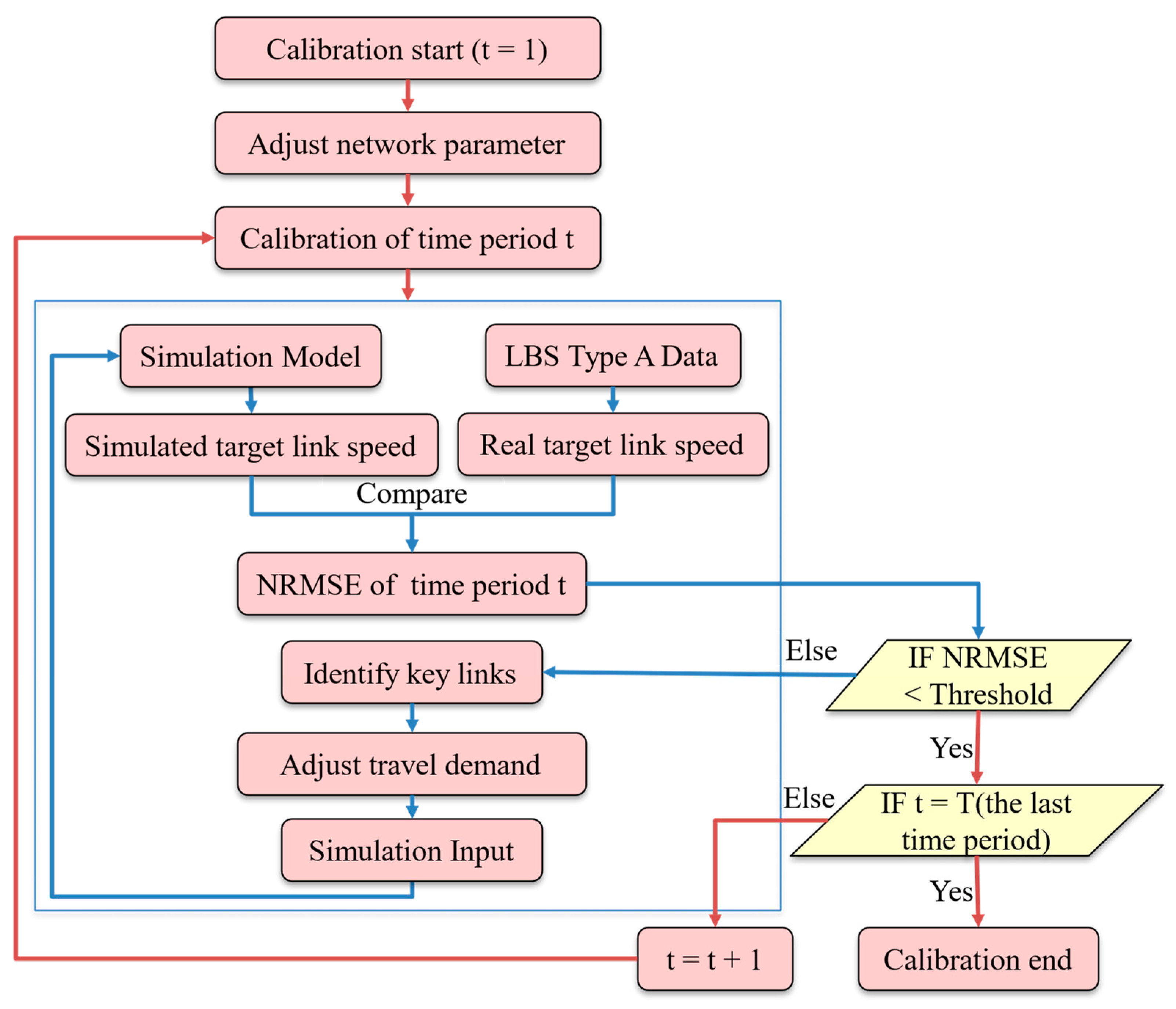
3.4.2. Simulation Model Calibration Method

The calibration goal is that NRMSEs are below a specified threshold for all periods. The process of simulation model calibration is shown in Figure 5.

First, the identification and correction of errors in road segment information are conducted: We start by loading the initial simulation demand over time onto the road network, obtaining simulation results for all time intervals, and assessing whether there are instances of generally higher or lower speeds compared to actual values over all or most time periods. This occurrence may stem from notable differences between the predetermined link capacity/speed limit and the actual functional value. During the link attribute calibration process, three links had significantly higher or lower simulated speeds than real-world observations. The speed limits of these links in the initial simulation (based on the preprocessing rule in Table 3 and Table 4) are inherently lower than the actual speeds. It could result from errors in the speed limit information of the original network data. In such cases, we use the street view feature of Amap to check their speed limit and make corrections accordingly. And for links where the simulated speeds are notably higher than the reality, we appropriately reduce their capacities to model real-world congestions.

After the aforementioned calibration steps, the identification and elimination of the universal deviation between the simulated link speeds and the actual link speeds have been accomplished, thus completing the calibration of the supply aspect of the simulation model. Subsequently, taking into account the time-dependency of traffic flow, the calibration of OD pairs on road segments is conducted in a time-specific manner to adjust the travel demand on the links. The following steps are involved:

Step 1: Calculation of overall error for the current time period. Commencing with the calibration of the first time period, we calculate the RMSE and NRSME between the average speeds of all links in the simulation and those in reality for the current time period t. If the NRSME falls below the threshold γ, it indicates that the error between the simulated average link speeds and the actual average speeds is within the permissible range for that time period. Subsequently, the travel demand for the fixed time period t is maintained, and calibration proceeds to the next time period (t = t + 1) until t = T (the last time period). However, if the NRSME exceeds the threshold γ, calibration for the current time period continues.

Step 2: Selection of key links for demand calibration. The deviation between the simulated and actual speeds is calculated as follows to obtain the deviation value $D{V}_{m,t}$ for each link during the current time period t.

$$D{V}_{m,t}=\left|{\log }_C{S}_{m,t}^{\prime }/S_{m,t}\right|$$

(6)

where $D{V}_{m,t}$ represents the deviation between the simulated and actual average speeds of link m during time period t, $S_{m,t}^{\prime }$ is the average speed of link m in the simulation during time period t, $S_{m,t}$ is the average speed of link m in reality during time period t, C is a deviation multiplier constant, set to 2 in this study. When the simulated and actual average speeds are identical, the deviation $D{V}_{m,t}$ is 0, whereas, when the simulated average speed is half or double the actual average speed, the deviation $D{V}_{m,t}$ is 1.

Subsequently, the K links with the largest deviations are selected from the set of target links. A small value of K means that calibration is only conducted on a few road segments within the target set, leading to a slow and lengthy calibration process. Conversely, a large value of K can result in excessive adjustment of OD flows due to their potential impact on multiple target road segments, potentially leading to issues such as over-adjustment and insignificant results. Therefore, through trials with various K values (including 5, 10, 20, 25, 30, and 50), this study evaluates the calibration effectiveness for the first time period. Considering both accuracy and efficiency, K is ultimately set to 20, slightly lower than half of the total number of target road segments (50). This setting aims to balance calibration effectiveness with practical convenience and can serve as a reference for other calibration studies.

Step 3: Calculating the rescaling factor for OD demand on key links. By analyzing the simulation’s travel path output files, the travel paths containing the identified critical roads are extracted, and the current demand for the critical OD pairs is further quantified. Adjustments to the travel demand on these roads are made based on the ratio of simulated link speeds to actual link speeds. Specifically, the rescaling factor for OD pairs on critical road segment m is calculated as follows:

$$F_{m,t}^{\prime }=\frac{S_{m,t}^{\prime }}{S_{m,t}}$$

(7)

where $F_{m,t}^{\prime }$ is the rescaling factor for OD pairs using key link m during time period t in the current iteration; $S_{m,t}^{\prime }$ and $S_{m,t}$ are the average speeds observed on link m during time period t from the simulation model and LBS data, respectively.

When the simulated link speed is higher than the actual speed, the ratio in the rescaling factor will be greater than 1, indicating smoother traffic flow on the same link in the simulation compared to reality. This implies that the current simulation underestimates the travel demand on this link, necessitating the expansion of demand to simulate more congested conditions. Conversely, when the simulated link speed is lower than the reality, the ratio will be less than 1, reflecting more congestion in the simulation than in reality. In this case, the current simulation overestimates the travel demand, requiring a reduction in demand to simulate smoother traffic.

Step 4: Determining the OD volume on key links for the next calibration iteration. During the calibration iterations, a coefficient that gradually decreases from 1 to 0 as the calibration process for the current time period progresses is introduced. This ensures efficient adjustments during the initial stages of calibration and finer, more stable adjustments later on. Based on the current number of vehicles (or OD pairs) using the key link during the current time period in the current simulation calibration iteration and its rescaling factor, the number of vehicles (or OD pairs) expected to use the key link during the same time period in the next calibration iteration is calculated as follows:

$$N_{it+1,m,t}^{\prime }=\left\{\begin{array}{c}{N}_{it,m,t}^{\prime }\ast \left[1+k\ast \left(F_{m,t}^{\prime }-1\right)\right], \hspace{1em}{F}_{m,t}^{\prime }>1\\ N_{it,m,t}^{\prime }\ast \left[1-k\ast \left(1-F_{m,t}^{\prime }\right)\right], \hspace{1em}{F}_{m,t}^{\prime }<1\end{array}\right.$$

(8)

where $F_{m,t}^{\prime }$ is the rescaling factor for the OD volume using key link m in time period $t$ during the current iteration $it$, $S_{m,t}$ and $S_{m,t}^{\prime }$ denote the average speeds of the link as observed from LBS data and in the simulation model, respectively. $N_{it+1,m,t}^{\prime }$ is the number of vehicles (or OD) that will use key link $m$ in time period $t$ during the next calibration iteration $it+1$ in simulation model, $N_{it,m,t}^{\prime }$ is the number of vehicles (or OD) that will use key link $m$ in time period $t$ during the current calibration iteration $it$ in simulation model, $k$ is a speed coefficient for the calibration process, gradually decreasing from 1 to 0 as the current time period calibration progresses.

During the process of demand resampling on links, we initially retain all travel demands passing through the key links within the current time period. Subsequently, we calculate the variation in demand by determining the difference between the new and original demand quantities. Based on this variation, we conduct a random sampling of the original travel demand set to generate a collection reflecting the changes in demand. This modified set is then merged with the existing travel demand set for the current time period. Notably, due to the limited coverage of LBS data, the calibration process infrequently involves the reduction in original LBS travel records. Instead, the focus of the demand reduction process is primarily on addressing excessive resampling on links. In such scenarios, all original LBS travel records and their corresponding demands are preserved, and the random sampling is solely applied to the modified demand set.

This comprehensive approach ensures the accuracy and reliability of the travel demand data, thereby enhancing the effectiveness of the simulation model. Additionally, we generally need a warming-up period before the initial calibration time period. This warming-up period does not require any calibration or statistical analysis.

3.5. LBS Missing Path Completion

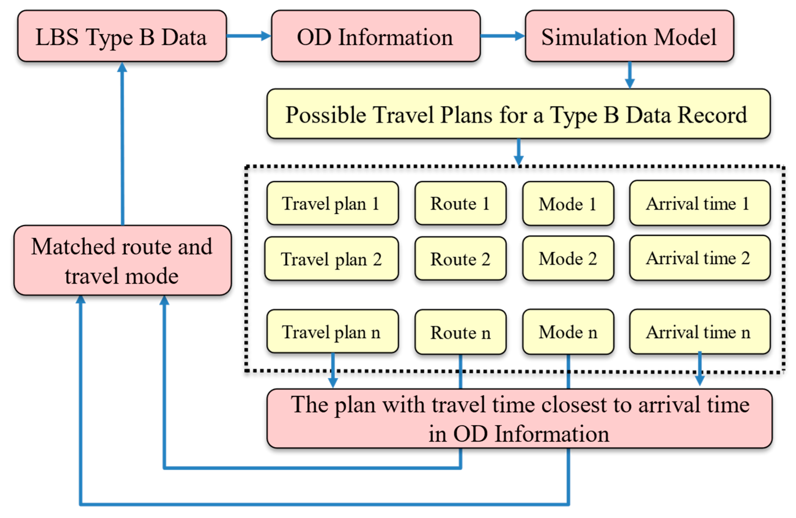
3.5.1. Completion of Missing Paths for LBS Sparse Trajectory Points

Completing missing personal travel path information can improve the accuracy of LBS data and enhance the robustness of travel decision-making studies. As discussed in Section 3.3, Type B data exhibit significant spatial-temporal gaps between trajectory points, resulting in multiple possible paths. Therefore, conducting missing path completion for Type B data becomes necessary. The known information in Type B LBS data mainly consists of the spatial-temporal information of OD (i.e., the coordinates and time of departure and arrival), with some containing travel mode information. Through a series of steps, including traffic assignment, time point alignment, and others, we have established a core process to complement the missing travel paths, forming the essence of this research. The entire LBS missing path completion process is shown in Figure 6, demonstrating every step from plan generation, through screening and filtering, to the final path completion.

Step 1: Generating travel plans with different route choices for travel demands. Since the original travel demands generated from these Type B LBS travel trajectory data do not specify the travel route information, we first generate the shortest S travel plans containing various possible shortest travel routes as the possible solution set for completing the missing paths based on simulation. When the value of S is too small, the travel solution set may not include the actual route selection. Conversely, when the value of S is too large, the efficiency of completion will decrease. Therefore, in this study, the value of S is set to 20 for paths with different degrees of deletion. In these travel plans, the planned departure time and location are consistent with the information of the starting O point in the Type B LBS travel demands. Similarly, the planned destination location is the same as the coordinate of the destination D point in the Type B LBS travel demands. The planned travel mode is consistent with the travel mode attribute of the Type B LBS travel demands. When the travel mode information in the original travel demand is unknown, the 20 possible travel routes generated include different route choices under various travel modes (private car, bus, and subway).

Step 2: Obtaining travel time for each route through simulation. The different travel routes under the travel demands are input into the calibrated simulation model, and the travel time corresponding to each travel route in the feasible solutions of the travel demands is obtained through simulation execution:

$$\left\{(p_{i,k,1},T_{{\mathrm{O}}_i,{\mathrm{D}}_k,1}^{\prime }), (p_{i,k,2},T_{{\mathrm{O}}_i,{\mathrm{D}}_k,2}^{\prime }),\dots , (p_{i,k,n},T_{{\mathrm{O}}_i,{\mathrm{D}}_k,n}^{\prime })\right\}$$

(9)

where $p_{i,k,1}$ represents the n-th shortest path between the origin ${\mathrm{O}}_i$ and the destination ${\mathrm{D}}_k$, and $T_{{\mathrm{O}}_i,{\mathrm{D}}_k,n}^{\prime }$ corresponds to the travel time of the path.

Step 3: Matching and completion of feasible travel paths. The travel time between the origin and destination of the original travel demand is calculated as the actual travel duration on the vehicle’s true path, shown as follows:

$${\mathrm{T}}_{{\mathrm{O}}_i,{\mathrm{D}}_k}={ \mathrm{t}}_{{\mathrm{D}}_k}-{\mathrm{t}}_{{\mathrm{O}}_i}$$

(10)

where ${\mathrm{T}}_{{\mathrm{O}}_i,{\mathrm{D}}_k}$ represents the actual travel time of the trip between the origin ${\mathrm{O}}_i$ and the destination ${\mathrm{D}}_k$ corresponding to the LBS data, ${\mathrm{t}}_{{\mathrm{D}}_k}$ is the time at which the travel demand is at ${\mathrm{D}}_k$, and ${\mathrm{t}}_{{\mathrm{O}}_i}$ is the time at which the travel demand starts at ${\mathrm{O}}_i$.

Next, the absolute difference between the travel time of all possible travel paths obtained from the simulation and the actual travel time is calculated, shown as follows:

$$\Delta {\mathrm{T}}_{{\mathrm{O}}_i,{\mathrm{D}}_k,n}=\left|{\mathrm{T}}_{{\mathrm{O}}_i,{\mathrm{D}}_k}-T_{{\mathrm{O}}_i,{\mathrm{D}}_k,n}^{\prime }\right|$$

(11)

where $\Delta {\mathrm{T}}_{{\mathrm{O}}_i,{\mathrm{D}}_k,n}$ is the absolute difference between the actual travel time and the simulated travel time between the origin ${\mathrm{O}}_i$ and the destination ${\mathrm{D}}_k$, $T_{{\mathrm{O}}_i,{\mathrm{D}}_k,n}^{\prime }$ is the travel time of the n-th travel path.

Then, we select the travel path $p_{i,k,n}$ corresponding to the minimum absolute difference in travel time $\Delta {\mathrm{T}}_{{\mathrm{O}}_i,{\mathrm{D}}_k,n}$ as the path completion result for the travel demand, and the travel mode $mod{e}_{\left(n\right)}$ corresponding to this path is used as the travel mode completion result when the travel mode is missing, shown as follows:

$$\Delta {\mathrm{T}}_{{\mathrm{O}}_i,{\mathrm{D}}_k}= \min \left(\Delta {\mathrm{T}}_{{\mathrm{O}}_i,{\mathrm{D}}_k,1}, \Delta {\mathrm{T}}_{{\mathrm{O}}_i,{\mathrm{D}}_k,2},\cdots , \Delta {\mathrm{T}}_{{\mathrm{O}}_i,{\mathrm{D}}_k,n} \right)$$

(12)

Furthermore, after the completion, we reassessed the average speed of the target links and calculated a new NRMSE value. If the path completion deteriorates the calibration results (the new error exceed the preset threshold), then we return to the calibration process and adjust OD demand again. This iterative and feedback mechanism ensures the continuous optimization and precision of the calibration and completion work in this study. Moreover, this study compared the changes in the average speed of the target road segments in the calibration model and found that the complementation and correction of Type B data had a minimal impact on the error between the traffic simulation model and the actual situation. In other words, the error of the adjusted model remained within the threshold set by this study (below 30%).

In theory, our method of completing missing paths ensures a high degree of matching between the complemented travel paths and the actual missing travel data in terms of the departure and arrival times, as well as locations. The completion process also strictly adheres to the real-world average road speeds. Therefore, the completed result will be more realistic and credible.

3.5.2. Evaluation of the Effectiveness of Missing Path Completion for LBS Data

To validate the accuracy of the travel mode completion results, this study randomly selected 2000 Type B LBS data records containing actual travel mode information for testing the travel mode completion process. Among them, 1000 records were for private vehicle travel, while the remaining 1000 were for public transportation. For each OD pair, this study generated 20 candidate paths, including both public transportation and private vehicle travel modes. The closest travel path selection and its corresponding travel mode were obtained using the method described in Section 4.2 and compared with the original recorded travel mode.

To evaluate the performance of the path completion method, this study designed the following validation strategy. Since Type B data inherently lack path information and cannot serve for validation, we intentionally introduce artificial missing paths within partial of Type A data. Specifically, for each complete Type A travel path, only the spatiotemporal information at the first and last nodes is retained, including the OD nodes locations and time information. The artificially omitted path information between these nodes is then used as a reference for validating the completed path. Using this method, this study constructed 10 subsets of Type A LBS data specifically designed for validating path completion performance. These subsets encompassed varying degrees of missingness, ranging from one missing link to nine missing links. Each level of missingness contained 200 data.

Similar to the process of path completion for Type B data, we obtain the simulated completion results of the validation set. Then, the performance of the completion effect is checked by comparing the overlap ratio between completed and actual paths. We calculate the link coincidence rate (LCR) and path length coincidence rate (PLCR), given as follows, as the performance metric of the completion method.

$$LC{R}_{{\mathit{P}}_{\mathit{L}}}=\frac{\left|P_S^{\prime }\cap P_L\right|}{\left|P_L\right|}$$

(13)

$$PLC{R}_{{\mathit{P}}_{\mathit{L}}}=\frac{{{\displaystyle \sum }}_{\mathit{s}\in \left(P_S^{\prime }\cap P_L\right)}{l}_s}{{{\displaystyle \sum }}_{\mathit{k}\in {\mathit{P}}_{\mathit{L}}}{l}_k}$$

(14)

where $LC{R}_{{\mathit{P}}_{\mathit{L}}}$ is LCR of the completion result, $PLC{R}_{{\mathit{P}}_{\mathit{L}}}$ is the PLCR of the completion result, $P_S^{\prime }\cap P_L$ is the overlapping links between the path $P_S^{\prime }$ obtained from the simulation model and the path $P_L$ obtained from LBS data. $s$ is the link common to both $P_S^{\prime }$ and $P_L$, and $k$ is link in $P_L$.

To demonstrate the performance of our DDSM, we compare the accuracy between our model and two baseline methods:

(a) Dual-driven simulation model (DDSM);

(b) Shortest path algorithm (SP), in which the shortest travel distance among the generated multiple paths is selected;

(c) Time-dependent shortest path algorithm (TDSP), in which the travel time for each link is calculated by dividing the link length by its speed limit, and then the path with the shortest travel time from among the multiple generated paths is selected.

4. Results

4.1. Data and Simulation Initialization

Based on the multi-modal simulation network and the travel plans/demand obtained from the LBS data, we construct the MATSim initial model. Under an operating system configured as Windows 10 and AMD64, with eight CPU cores, and a maximum simulated memory set at 15,000 MB, the average simulation time per iteration is 6.01 s. After 50 iterations, the scores of the agent population tend to be stable, indicating the completion of simulation initialization.

4.2. Simulation Calibration Results

Figure 7 represents the variations in RMSE and NRMSE, respectively, between simulated and real-world space mean speeds of the target links in the first time period. Overall, the errors show a decreasing trend along with iterations, and reach the threshold at around 18 iterations. We can observe a slight increase in RMSE and NRMSE during the eleventh calibration iteration. This could result from the insensitivity between speed and traffic volume so that some links may have over-calibration. Nevertheless, our calibration process accurately identifies and corrects such over-calibration, ensuring the accuracy of the final results. In the subsequent process, the error values resumed their downward trend.

Figure 8 depicts the variations in RMSE and NRMSE, respectively, between simulated and real-world space mean speeds of the target links across all time periods. Similarly, the errors exhibit a decreasing trend and become stable after around 380 iterations. During the intermediate stages of calibration, there are sharp decreases in error values to varying degrees. This is because the calibration process is performed on a per-time-period basis, and as the model calibration for the current time period proceeds, the rate of error reduction gradually slows down. Once the error for the current time period satisfies the threshold λ, we fix the travel demand for that period and proceed to calibrate the next time period. The transition between calibration periods results in a sudden drop in error, followed by a gradual slowdown as the calibration iterations continue. Notably, as the number of iterations for each time period increases, the rate of errors decreases more rapidly, indicating that subsequent time periods are easier to calibrate than previous periods.

Regarding the speed of the calibration iteration process, the average time spent per iteration during the calibration of the first time slice in this study was only 44 s. As the travel demand was scaled up, the overall travel plan for the simulation increased, resulting in a corresponding increase in the computation time for the average travel time of road segments within the simulation. Consequently, the final calibration iteration for the last time slice took 155 s, and the entire calibration process for the travel demand of the simulation model lasted approximately 11 h.

The variations in errors between the simulated and real-world space mean the speeds of the target links for each time period before and after calibration and the variations in errors across all time periods are presented in

Table 5. Comparison of RMSE and NRMSE between simulated and real-world space mean speeds of the target links before and after calibration.

Time Period	Initial RMSE	Final RMSE	Initial NRMSE	Final NRMSE
1	4.117	1.951	0.442	0.209
2	4.760	1.912	0.572	0.230
3	5.071	2.156	0.649	0.276
4	5.379	2.106	0.732	0.287
5	5.510	1.718	0.724	0.226
6	5.440	1.756	0.722	0.233
7	5.424	2.063	0.670	0.255
8	4.974	1.801	0.618	0.224
All	5.217	1.939	0.638	0.241

. Through a comparative analysis, it is clearly observed that there is a significant improvement in error during the calibration process. After calibrating the simulation model, the RMSE of the average speed for the target road segment across all time periods decreased from 5.217 m/s to 1.939 m/s. The NRMSE for each individual time period was reduced to below 30%, while the overall NRMSE across all time periods decreased from 63.9% to 24.1%. In the final iteration, the travel demand is 296,906 trips. Compared to all the original 68,850 data from Type A and Type B data, we can conclude that the original data significantly underestimated the actual transportation demand, indirectly indicating the limited coverage of LBS user data.

4.3. Results of Path Completion

Among the 1000 car mode data records, we complete 994 paths, of which 953 paths are correctly identified as car mode, which achieves an accuracy rate of 95.3% in recognizing car mode. But 41 paths are wrongly identified as the public transit mode. The potential reason for the misidentification of travel modes is that for these travel records, the time difference in travel duration between choosing private car mode and choosing public transportation during the departure and arrival time periods is not very significant.

In the case of 1000 public transit mode data records, we identify the public transit mode for only 616. One possible reason is that we may mistakenly identify many public transportation trips with long first-/last-mile distances as the car mode. The first-/last-mile distance can influence people’s choice of public transit mode. To address such an issue, we specify a radius of 1000 m for searching nearby stations of each trip’s origin and destination. Hence, public transit trips with excessive walking distances before and after boarding and lengthy transfer distances are excluded.

The performance of the three path completion methods across ten testing sets is shown in Figure 9. The accuracy of all three methods decreases with the increase in missing path numbers. As travel routes become longer (involving more links), the transportation system’s uncertainty increases, making it difficult for travelers to perceive and choose the shortest path. In other words, the shortest-path completion methods face challenges when simulating human behavior on long-distance trips. Therefore, the accuracy of the shortest path algorithm is highly sensitive to the completeness of the data.

After separately weighting the quantities and lengths of missing road segments,

Table 6. Effectiveness of different path completion algorithms after weighting across ten testing sets.

Performance	DDSM	SP	TDSP
LCR	84.78% (±0.444%)	77.98% (±0.599%)	81.96% (±0.489%)
PLCR	85.02% (±0.449%)	79.19% (±0.683%)	82.92% (±0.455%)
AVG	84.90% (±0.438%)	78.59% (±0.648%)	82.44% (±0.465%)

presents the comprehensive LCR and PLCR values for the DDSM and two baseline algorithms, as well as the averages of LCR and PLCR. The numbers outside the parentheses represent the average metrics derived from 10 subsets, while the numbers inside the parentheses indicate the standard deviations for these subsets.

Compared to two comparative algorithms, the LCR values of DDSM separately increase by 6.80% and 2.82%, while the PLCR values increase by 5.83% and 2.10%, respectively. Furthermore, the comprehensive averages of LCR and PLCR for DDSM improved by 6.31% and 2.46%, respectively, indicating its overall superiority. Notably, the performance of DDSM is even more stable across all ten subsets, further validating its robustness and reliability. This stability across multiple subsets underscores the significant advantage of the proposed DDSM in terms of accuracy, making it a promising approach for missing path completion.

5. Conclusions

This study proposes a dual-driven simulation model (DDSM) based on LBS data and traffic simulation to achieve multi-modal simulation modeling and calibration as well as missing LBS data completion. The DDSM approach explores and utilizes LBS data, a novel but underused data source in simulation model development and calibration. Relying on the route/mode choice results from the calibrated model, the missing paths of LBS data are completed by matching the departure and arrival times and locations of simulated trip paths and those of observed trips. The applicability of this method was validated by applying it to an urban area in Hangzhou, China. When utilizing an LBS data and calibration framework in our paper, the model error quickly falls within the permissible range (24%). The results demonstrate the excellent performance of the proposed approach in identifying private car travel modes, achieving an accuracy rate of 95.3%, and outperforming baseline LBS completion algorithms with respective increases of 6.31% and 2.46% in completion accuracy. According to the case study, the completion process adheres to the real-world average road speeds, making it more realistic, and thus the identification of travel modes and paths has a high accuracy. This implies the advantages of our DDSM method in urban-level traffic modeling and the large-scale completion of missing LBS data.

Future work should focus on improving the following aspects of implementation. Due to data limitations, the calibration process used Space Mean Speed for calibration. Subsequent research can use more abundant road condition information (e.g., traffic flow, and speed) for a more precise simulation model calibration. Due to the lack of public transport trip records and route selection in the data itself, we can only output possible solutions for public transit route selection through the model, making a rough screening using departure and arrival time. In the future, other data sources will be used for further testing and verification.

References

1. Colak, S.; Lima, A.; González, M.C. Understanding congested travel in urban areas. Nat. Commun. 2016, 7, 10793. [Google Scholar] [CrossRef] [PubMed]
2. Ehmke, J.F.; Campbell, A.M.; Thomas, B.W. Data-driven approaches for emissions-minimized paths in urban areas. Comput. Oper. Res. 2016, 67, 34–47. [Google Scholar] [CrossRef]
3. Vazifeh, M.M.; Santi, P.; Resta, G.; Strogatz, S.H.; Ratti, C. Addressing the minimum fleet problem in on-demand urban mobility. Nature 2018, 557, 534–538. [Google Scholar] [CrossRef]
4. Xiao, Y.; Yang, M.F.; Zhu, Z.; Yang, H.; Zhang, L.; Ghader, S. Modeling indoor-level non-pharmaceutical interventions during the COVID-19 pandemic: A pedestrian dynamics-based microscopic simulation approach. Transp. Policy 2021, 109, 12–23. [Google Scholar] [CrossRef] [PubMed]
5. Chen, X.Q.; Xiong, C.F.; He, X.; Zhu, Z.; Zhang, L. Time-of-day vehicle mileage fees for congestion mitigation and revenue generation: A simulation-based optimization method and its real-world application. Transp. Res. Part C-Emerg. Technol. 2016, 63, 71–95. [Google Scholar] [CrossRef]
6. Gao, Y.H.; Qu, Z.W.; Song, X.M.; Yun, Z.Y. Modeling of urban road network traffic carrying capacity based on equivalent traffic flow. Simul. Model. Pract. Theory 2022, 115, 102462. [Google Scholar] [CrossRef]
7. Zhu, Z.; Xiong, C.F.; Chen, X.Q.; He, X.; Zhang, L. Integrating mesoscopic dynamic traffic assignment with agent-based travel behavior models for cumulative land development impact analysis. Transp. Res. Part C-Emerg. Technol. 2018, 93, 446–462. [Google Scholar] [CrossRef]
8. Saw, K.; Katti, B.K.; Joshi, G. Literature Review of Traffic Assignment: Static and Dynamic. Int. J. Transp. Eng. 2015, 2, 339–347. [Google Scholar]
9. de Souza, F.; Verbas, O.; Auld, J. Mesoscopic Traffic Flow Model for Agent-Based Simulation. In Proceedings of the 10th International Conference on Ambient Systems, Networks and Technologies (ANT)/2nd International Conference on Emerging Data and Industry 4.0 (EDI40), Leuven, Belgium, 29 April–2 May 2019; pp. 858–863. [Google Scholar]
10. Griggs, W.M.; Ordóñez-Hurtado, R.H.; Crisostomi, E.; Häusler, F.; Massow, K.; Shorten, R.N. A Large-Scale SUMO-Based Emulation Platform. IEEE Trans. Intell. Transp. Syst. 2015, 16, 3050–3059. [Google Scholar] [CrossRef]
11. Morency, C. The ambivalence of ridesharing. Transportation 2007, 34, 239–253. [Google Scholar] [CrossRef]
12. Xie, M.Q.; Cheng, W.; Gill, G.S.; Zhou, J.; Jia, X.D.; Choi, S. Investigation of hit-and-run crash occurrence and severity using real-time loop detector data and hierarchical Bayesian binary logit model with random effects. Traffic Inj. Prev. 2018, 19, 207–213. [Google Scholar] [CrossRef] [PubMed]
13. Friedrich, M.; Immisch, K.; Jehlicka, P.; Otterstätter, T.; Schlaich, J. Generating Origin-Destination Matrices from Mobile Phone Trajectories. Transp. Res. Rec. 2010, 2196, 93–101. [Google Scholar] [CrossRef]
14. Munizaga, M.A.; Palma, C. Estimation of a disaggregate multimodal public transport Origin-Destination matrix from passive smartcard data from Santiago, Chile. Transp. Res. Part C-Emerg. Technol. 2012, 24, 9–18. [Google Scholar] [CrossRef]
15. Gurram, S.; Sivaraman, V.; Apple, J.T.; Pinjari, A.R. Agent-based modeling to simulate road travel using Big Data from smartphone GPS: An application to the continental United States. In Proceedings of the IEEE International Conference on Big Data (Big Data), Los Angeles, CA, USA, 9–12 December 2019; pp. 3553–3562. [Google Scholar]
16. Zhang, L.; Yang, W.C.; Wang, J.M.; Rao, Q. Large-Scale Agent-Based Transport Simulation in Shanghai, China. Transp. Res. Rec. 2013, 2399, 34–43. [Google Scholar] [CrossRef]
17. Kim, K.; Pant, P.; Yamashita, E. Integrating travel demand modeling and flood hazard risk analysis for evacuation and sheltering. Int. J. Disaster Risk Reduct. 2018, 31, 1177–1186. [Google Scholar] [CrossRef]
18. Qasim, Z.; Ziboon, A.R.; Falih, K. TransCad analysis and GIS techniques to evaluate transportation network in Nasiriyah city. In Proceedings of the 3rd International Conference of Buildings, Construction and Environmental Engineering (BCEE), Sharm el Sheikh, Egypt, 23–25 October 2017. [Google Scholar]
19. Jacyna, M.; Wasiak, M.; Klodawski, M.; Golebiowski, P. Modelling of Bicycle Traffic in the Cities Using VISUM. In Proceedings of the 10th International Scientific Conference on Transportation Science and Technology (TRANSBALTICA), Vilnius, Lithuania, 4–5 May 2017; pp. 435–441. [Google Scholar]
20. Balmer, M.; Rieser, M.; Meister, K.; Charypar, D.; Lefebvre, N.; Nagel, K.; Axhausen, K. MATSim-T: Architecture and simulation times. In Multi-Agent Systems for Traffic and Transportation Engineering; IGI Global: Hershey, PA, USA, 2009; pp. 57–78. [Google Scholar]
21. Chen, X.Q.; Zhu, Z.; Zhang, L. Simulation-based optimization of mixed road pricing policies in a large real-world network. In Proceedings of the Current Practices in Transport: Appraisal Methods, Policies and Models, 42nd European Transport Conference Selected Proceedings, Goethe Univ, Frankfurt, Germany, 29 September–1 October 2014; pp. 215–226. [Google Scholar]
22. Chen, X.Q.; Zhang, L.; He, X.; Xiong, C.F.; Li, Z.H. Surrogate-Based Optimization of Expensive-to-Evaluate Objective for Optimal Highway Toll Charges in Transportation Network. Comput.-Aided Civ. Infrastruct. Eng. 2014, 29, 359–381. [Google Scholar] [CrossRef]
23. Noh, H.; Chiu, Y.C.; Zheng, H.; Hickman, M.; Mirchandani, P. Approach to Modeling Demand and Supply for a Short-Notice Evacuation. Transp. Res. Rec. 2009, 2091, 91–99. [Google Scholar] [CrossRef]
24. Park, B.B.; Won, J.; Yun, I. Application of microscopic simulation model calibration and validation procedure—Case study of coordinated actuated signal system. In Proceedings of the 85th Annual Meeting of the Transportation-Research-Board, Washington, DC, USA, 22–26 January 2006; pp. 113–122. [Google Scholar]
25. Gao, Y.H.; Qu, Z.W.; Song, X.M.; Yun, Z.Y.; Zhu, F. Coordinated perimeter control of urban road network based on traffic carrying capacity model. Simul. Model. Pract. Theory 2023, 123, 102680. [Google Scholar] [CrossRef]
26. Gulhan, G.; Ceylan, H.; Özuysal, M.; Ceylan, H. Impact of utility-based accessibility measures on urban public transportation planning: A case study of Denizli, Turkey. Cities 2013, 32, 102–112. [Google Scholar] [CrossRef]
27. Tang, J.Y.; McNabola, A.; Misstear, B.; Caulfield, B. An evaluation of the impact of the Dublin Port Tunnel and HGV management strategy on air pollution emissions. Transp. Res. Part D-Transp. Environ. 2017, 52, 1–14. [Google Scholar] [CrossRef]
28. Basavaraj, V.; Noyes, D.; Fiondella, L.; Lownes, N. Mitigating the Impact of Transportation Network Disruptions on Evacuation. In Proceedings of the IEEE International Symposium on Technologies for Homeland Security (HST), Waltham, MA, USA, 14–16 April 2015. [Google Scholar]
29. Ahmed, F.; Hawas, Y.E. An integrated real-time traffic signal system for transit signal priority, incident detection and congestion management. Transp. Res. Part C-Emerg. Technol. 2015, 60, 52–76. [Google Scholar] [CrossRef]
30. Feng, Y.H.; Head, K.L.; Khoshmagham, S.; Zamanipour, M. A real-time adaptive signal control in a connected vehicle environment. Transp. Res. Part C-Emerg. Technol. 2015, 55, 460–473. [Google Scholar] [CrossRef]
31. Li, Y.F.; Song, Y.; Zheng, T.X.; Feng, H.Z. TransModeler based implementation of autonomous vehicular platoon control. In Proceedings of the 29th Chinese Control And Decision Conference (CCDC), Chongqing, China, 28–30 May 2017; pp. 4087–4092. [Google Scholar]
32. Song, Z.J.; Wang, H.Z.; Sun, J.; Tian, Y. Experimental Findings with VISSIM and TransModeler for Evaluating Environmental and Safety Impacts using Micro-Simulations. Transp. Res. Rec. 2020, 2674, 566–580. [Google Scholar] [CrossRef]
33. Zegeye, S.K.; De Schutter, B.; Hellendoorn, J.; Breunesse, E.A.; Hegyi, A. Integrated macroscopic traffic flow, emission, and fuel consumption model for control purposes. Transp. Res. Part C-Emerg. Technol. 2013, 31, 158–171. [Google Scholar] [CrossRef]
34. Sewall, J.; Wilkie, D.; Lin, M.C. Interactive Hybrid Simulation of Large-Scale Traffic. ACM Trans. Graph. 2011, 30, 1–12. [Google Scholar] [CrossRef]
35. Hörl, S.; Balac, M. Synthetic population and travel demand for Paris and Ile-de-France based on open and publicly available data. Transp. Res. Part C-Emerg. Technol. 2021, 130, 103291. [Google Scholar] [CrossRef]
36. Patel, V.; Chaturvedi, M.; Srivastava, S. Comparison of SUMO and SiMTraM for Indian Traffic Scenario Representation. In Proceedings of the 11th International Conference on Transportation Planning and Implementation Methodologies for Developing Countries (TPMDC), Mumbai, India, 10–12 December 2014; pp. 400–407. [Google Scholar]
37. Onelcin, P.; Mutlu, M.M.; Alver, Y. Evacuation plan of an industrial zone: Case study of a chemical accident in Aliaga, Turkey and the comparison of two different simulation softwares. Saf. Sci. 2013, 60, 123–130. [Google Scholar] [CrossRef]
38. Yang, J.H.; Sun, J. Vehicle path reconstruction using automatic vehicle identification data: An integrated particle filter and path flow estimator. Transp. Res. Part C-Emerg. Technol. 2015, 58, 107–126. [Google Scholar] [CrossRef]
39. Sun, H.Z.; Jiang, P.; She, Q.S.; Yu, C.; Lin, H.Z.; Wu, X.; Lin, G. Excessive-emission vehicles real-time track matching algorithm based on road network topology and weights. In Proceedings of the 38th Chinese Control Conference (CCC), Guangzhou, China, 27–30 July 2019; pp. 6325–6332. [Google Scholar]
40. Wang, L.F. Study on Technology and Method of Tracking Survey of Running Vehicles Based on Plate Number. PhD Thesis, Chang’an University, Xian, China, 2013. [Google Scholar]
41. Ruan, S.B.; Wang, F.J.; Ma, D.F.; Jin, S.; Wang, D.H. Vehicle trajectory extraction algorithm based on license plate recognition data. J. Zhejiang Univ. Eng. Sci. 2018, 52, 836–844. [Google Scholar]
42. Cao, Q.; Ren, G.; Li, D.W.; Ma, J.S.; Li, H.J. Semi-supervised route choice modeling with sparse Automatic vehicle identification data. Transp. Res. Part C-Emerg. Technol. 2020, 121, 102857. [Google Scholar] [CrossRef]
43. Jafari, A.; Both, A.; Singh, D.; Gunn, L.; Giles-Corti, B. Building the road network for city-scale active transport simulation models. Simul. Model. Pract. Theory 2022, 114, 102398. [Google Scholar] [CrossRef]
Figure 1. Flowchart of the dual-driven simulation model.
Applsci 14 04366 g001
Figure 2. Multi-model network and public transportation routes distribution.
Applsci 14 04366 g002
Figure 3. Illustration of model initialization.
Applsci 14 04366 g003
Figure 4. Distribution of links to be calibrated (green) in the multi-model network.
Applsci 14 04366 g004
Figure 5. Iterative calibration process.
Applsci 14 04366 g005
Figure 6. Path completion method.
Applsci 14 04366 g006
Figure 7. Error variation between the space mean speeds of the target links in simulation and reality in the first period (7:00–7:15): (a) the variations in RMSE between simulated and real-world space mean speeds of the target links in the first time period; (b) the variations in NRMSE between simulated and real-world space mean speeds of the target links in the first time period.
Applsci 14 04366 g007
Figure 8. Variation in error between the space mean speeds of the target links in simulation and reality in all time periods: (a) the variations in RMSE between simulated and real-world space mean speeds of the target links in all time periods; (b) the variations in NRMSE between simulated and real-world space mean speeds of the target links in all time periods.
Applsci 14 04366 g008
Figure 9. Comparative analysis of LCR and PLCR in path completion algorithms across ten testing sets: (a) comparative evaluation of LCR among diverse path completion algorithms; (b) comparative evaluation of PLCR among diverse path completion algorithm.
Applsci 14 04366 g009